Methodology for Measuring Greenhouse Gas Emissions from Agricultural Soils Using Non-isotopic Techniques

Abstract

Several approaches exist for measuring greenhouse gases (GHGs), mainly CO₂, N₂O, and CH₄, from soil surfaces. The principle methods that are used to measure GHG from agricultural sites are chamber-based techniques. Both open and closed chamber techniques are in use; however, the majority of field applications use closed chambers. The advantages and disadvantages of different chamber techniques and the principal steps of operation are described. An important part of determining the quality of the flux measurements is the storage and the transportation of the gas samples from the field to the laboratory where the analyses are carried out. Traditionally, analyses of GHGs are carried out via gas chromatographs (GCs). In recent years, optical analysers are becoming increasingly available; these are user-friendly machines and they provide a cost-effective alternative to GCs. Another technique which is still under development, but provides a potentially superior method, is Raman spectroscopy. Not only the GHGs, but also N₂, can potentially be analysed if the precision of these techniques is increased in future development. An important part of this chapter deals with the analyses of the gas concentrations, the calculation of fluxes, and the required safety measures. Since non-upland agricultural lands (i.e. flooded paddy soils) are steadily increasing, a section is devoted to the specificities of GHG measurements in these ecosystems. Specialised techniques are also required for GHG measurements in aquatic systems (i.e. rivers), which are often affected by the transfer of nutrients from agricultural fields and therefore are an important indirect source of emission of GHGs. A simple, robust, and more precise method of ammonia (NH₃) emission measurement is also described.

2.1 Introduction

Given the complexity of emissions, process-based models are not able to accurately estimate daily fluxes or the variations in fluxes due to variations in management practices. This limits our understanding of the factors affecting greenhouse gas (GHG) emissions and eventually restricts the development of agricultural management options that minimise GHG emissions. The Intergovernmental Panel on Climate Change (IPCC) requires local data based on field studies. Estimation of emission factors (EF) along with quantification of EF-associated physical, chemical, and biological processes that produce CH₄ and N₂O is required for field-scale GHG measurements. Field measurement of GHG is the basis of GHG flux estimates and a means of evaluating potential countermeasures for reducing emissions (Minamikawa et al. 2015). Several approaches exist for measuring GHG fluxes from soil surfaces. The two most important approaches are chamber-based methods and micrometeorological techniques (Denmead 2008; Oertel et al. 2012) (Chap. 4); more sophisticated approaches include space and airborne measurements.

Micrometeorological techniques usually integrate much larger surface areas in comparison to chamber-based techniques, thereby substantially reducing spatial variability problems that are inherent to chamber-based methods (Mosier 1990). Micrometeorological techniques are often more expensive, require special analytical instruments, and need knowledge and expertise that are largely not available in most developing countries. There is also a third technique that could be used for gas flux estimation–the measurement of gas concentration in different layers of soil. Information about gas concentration in a soil profile can also be used for gas flux prediction (Chirinda et al. 2014; Kammann et al. 2001). However, this technique requires additional information on soil physical and chemical properties, including hydraulic characteristics, to calculate GHG fluxes based on gas diffusion in the soil matrix (Diel et al. 2019). Therefore, in most instances, chamber-based methods have been used to study GHG fluxes from agricultural soils. Nonetheless, in combination with chamber-based techniques, soil profile techniques can provide valuable additional information to explain and analyse GHG emissions from the soil surface (Müller et al. 2004).

2.2 Chamber-Based Methods

The great majority of GHG emission studies published in the past three decades have used chamber-based techniques–in particular, non-flow-through, non-steady-state chambers (Rochette 2011). These methods have been described in detail in several excellent review papers (De Klein and Harvey 2012; Hutchinson and Livingston 1993; Hutchinson and Rochette 2003; Mosier 1989). The following text mainly comes from these reviews that precisely address the topic and represent a comprehensive overview of the method. In addition to information from the literature, experimental data and our own experience with field gas flux determination will also be presented.

Mosier (1990) characterised three basic chamber-based techniques: open soil chambers (open dynamic chambers) that use flow-through air circulation, closed soil chambers with closed-loop air circulation (closed dynamic chambers), or no air circulation (static closed chambers).

2.2.1 Advantages and Disadvantages of Closed Chamber-Based Methods

The closed chamber technique has several advantages (Mosier 1990; Oertel et al. 2016), including the following:

• Closed chambers are simple and inexpensive to construct from various materials in different designs, shapes, and sizes, which makes it easier to find the type best suited for a given task.

• Operation of chambers and the measurement are simple, and therefore the method provides an opportunity to measure GHG from different locations at different times with the same equipment and personnel.

• Closed chambers can measure very low rates of GHG fluxes for pasture, cropland, rice paddy, wetland, drain, and ditches in a short period of time (from 30 min to 1 h), without the need for electrical supply.

The closed chamber technique, however, has some limitations:

• Increasing gas concentrations in the enclosed headspace leads to a decrease in the concentration gradient and therefore a reduction in gas diffusion, causing non-linear fluxes between the soil and the air. However, suppression of fluxes due to increased gas concentration in the headspace can be minimised by reducing the enclosure period.

• Closed chambers alter (or even eliminate) fluctuations of atmospheric pressure; however, special vents can equilibrate air pressure inside and outside of the chamber (Hutchinson and Mosier 1981; Mosier 1989).

• Temperature changes either in the soil or in the atmosphere within the chamber can occur. Such temperature differences within and outside the chamber are able to be reduced by covering the chamber with a reflective and insulating material (Mosier 1990; Šimek et al. 2014).

In summary, closed-chamber methods represent an inexpensive and easy to use technique, suitable for the determination of GHG fluxes between the soil and the atmosphere from a wide range of agroecosystems. However, several aspects must be considered when using the closed chamber-based methods, including the following:

• (i) Experimental design (design of the field experiment, number of replicated plots, plot size, etc.),

• (ii) Chamber construction (easy to use, easy to transport, but still robust enough to be repeatedly used without being easily damaged. The material used to construct the chamber should be inert and not emitting gases or allow diffusion through the material, but the material can be opaque or transparent),

• (iii) Sampling strategy (frequency of gas sampling, sample volume, number of samples, soil sampling in addition to gas sampling),

• (iv) Storage technique (vials for gas sample storage and transportation to laboratory, storage before analysis together with standards stored in the same way),

• (v) Analytical equipment (gas analysers such as gas chromatograph, CRDS (Cavity Ring-Down Spectroscopy) analyser), and

• (vi) Data analysis and interpretation (checking for linearity of gas concentration change over time in chambers during measurements. Also, checking for abnormal data points and proper statistical analysis).

Some of the problems with field GHG flux measurements are the large spatial variability of gas fluxes, and the high and often unpredictable temporal changes of fluxes. Other problems associated with field GHG flux measurements include the following:

• (i) Plants: Sometimes, it is difficult to deal with plants in gas collecting chambers due to their size. So, special chambers need to be designed (such as chambers for a maize field). Plants often consume (and produce) gases (e.g. CO₂, CH₄, and N₂O). Plants also transpire and influence the humidity in the chamber and movement of gases in the soil matrix, e.g. dissolved gas via the transpiration stream.

• (ii) Animals: It is difficult (if not impossible) to protect the chambers in areas grazed from damage by cattle and other animals. Permanent chambers can be easily damaged and can also cause injuries to animals.

• (iii) Technical and practical challenges: The large size of a field to be investigated, the frequent long-distance travel to the field, the large number of chambers to be moved around in the field, and a high requirement for manpower for proper GHG sampling.

2.2.2 Principles and Applications of Chamber-Based Techniques for Gas Flux Measurement

There is no best technique for GHG flux determination; each technique has its advantages and disadvantages, and no single approach is applicable for all conditions or purposes. An excellent overview of the principles and applications of chamber-based techniques for gas flux measurements was provided by Livingston and Hutchinson (1995). The following text is based on that publication and provides selected information, for practical reasons not every publication mentioned by the authors in their text is cited. More details and references can be found by Livingston and Hutchinson (1995). Some data and experiments taken from Šimek et al. (2014) are also included in this chapter. More recent developments in chamber-based techniques for N₂O flux measurements are discussed and summarised in De Klein and Harvey (2012) and Oertel et al. (2016). The factors causing high temporal and spatial variabilities in GHG emissions are outlined in the following sections.

2.2.3 Gas Exchange Processes

Rates of gas exchange between the soil and the atmosphere are usually extremely variable in time and space, making the determination of gas fluxes very complicated and challenging. Movement of gas molecules is due to either mass flow (advective transport) or molecular diffusion. Diffusive transport is described by Fick’s law and affected by gas permeability, i.e. the ease with which gases move through soil, varies over several orders of magnitude in relation to the shape, size, orientation of the soil pores and soil water content. Advective transport of gas occurs in response to a difference in total pressure between the soil air and the atmosphere, which is described by Darcy’s law. Water substantially affects the movement of gases in soil. Diffusivity of gases is about 10⁴ times smaller in water than in air (although the rates differ for different gases). Plants influence the exchange of gases; typically, the presence of plants results in increases in gas fluxes from and to the soil. Plants (mainly vascular plants) function as a direct pathway for the flow of trace gases through (often specialised) plant tissues (aerenchyma system); plants also alter conditions in the rhizosphere and therefore directly or indirectly influence gas formation and transport. Moreover, plants also consume and produce several gases, including CH₄ (Liu et al. 2015) or N₂O (Müller 2003). From a practical point of view, the presence of plants usually makes the gas flux determination even more challenging in comparison with bare soil.

2.2.4 Chamber Types

There are many types of closed/static chambers, typically developed by researchers for specific purposes (De Klein and Harvey 2012; Oertel et al. 2016; Saggar et al. 2007). The chambers may be made from various materials, including metals, plastics, and glass, and can have different designs, sizes, shapes, and volumes; chambers as small as 50 cm³ and as large as ca 1 m³ have been used for field flux determination from the soil surface. Obviously, chamber materials should be chemically inert, and thus, neither react with the gases being measured nor emit any contaminants. Recommended materials therefore include stainless steel, aluminium, and glass, while the use of polycarbonate, polyethylene, methyl methacrylate, and polyvinyl chloride should be checked for their suitability before use. The schematic diagram of the most common metal chamber is shown in Plate 2.1. This is similar to the design proposed by De Klein and Harvey (2012).

Plate 2.1

A schematic diagram a of three parts base frame, extension or enlargement and top lid with GHG sampling ports, a complete metal closed chamber in the paddy field (b), and specially designed chamber for maize plants (c and d)

Metal chambers, as shown in Plate 2.1, represent the best choice for many reasons. Metals are not permeable to gases and are inert if materials such as stainless steel are used and can be manufactured in local workshops. The type of material used is important because galvanised steel or normal steel may alter the soil conditions by releasing zinc and iron ions that have the potential to affect microbial activity; thus, it is recommended to use stainless steel. However, when compared to plastic chambers, they can be more expensive, heavier, and less available. Also, insulation is required to minimise temperature fluctuations inside the chamber which in turn would affect fluxes of GHG’s, and microbial processes that drive their production. Metal chambers typically consist of two or three parts: the bottom part (also called the base, frame, or soil collar/gutter), the top part (i.e. the chamber), and perhaps a suitable extension (Plate 2.1). The bottom part (frame) should be inserted into the soil at least 2 weeks before the first sampling and permanently installed to minimise soil disturbances effects. Chambers shall be insulated (e.g. using foam or polystyrene with reflective foils) to avoid unnatural heating during chamber closure. This allows repeated gas flux measurements in the same place, e.g. during the whole season. The two/three-part chamber design is strongly recommended, as the disturbances of soils prior to the measurements are eliminated. This, however, means that the frame should ideally be placed into the soil a few weeks before the measurements commence (De Klein and Harvey 2012; Oertel et al. 2016). Precautions should be taken in grazed sites so that neither the chamber nor the animals are endangered.

Plastic chambers have often been used for GHG flux determination (Plate 2.2a, b) (Zaman et al. 2009). The most critical issue for this type of chamber is the nature of the plastic used for making the chamber. Most plastic materials show permeability for gases, as well as the ability to emit some gases or react with them, e.g. hydrocarbons. The advantages of using plastic are (among others) the general availability, easiness to work with, low weight, and able to easily glue different parts together. Plastic chambers consist of two parts (a plastic vessel without a base/collar/gutter) and a lid. The plastic vessel is usually inserted into the soil at least 2–3 days prior to the flux measurement. For gas sampling, a lid containing a gas sampling port (rubber septum) connected to a three-way valve is carefully placed on top of the vessel using a gas-tight seal (Plate 2.2a, b). After gas samples are collected, the lid is removed. Plastic chambers can be either transparent or opaque.

Plate 2.2

Plastic chamber made up of two parts: vessel and lid for measuring greenhouse gas emission from a pasture soil and b arable and vegetable croplands

Glass chambers have been used less frequently, although the material (glass) is probably the best material to use, considering the inertness and the low gas permeability. However, glass is fragile which makes it very problematic to work with. Therefore, there are more disadvantages than advantages to use glass chambers. Still, one type of glass chambers has been tested for gas flux measurements (Plate 2.3). The major disadvantage of this chamber type is the limited size of the bottles available. Bottle volume is usually between 100 and 2000 cm³, and surface area covered by the chamber is less than 100 cm², which is too small for most uses. Glass chambers consist of a single part (without a base/collar/gutter) and are transparent.

Plate 2.3

Glass chamber consists of only one part (Šimek, personal communication) for measuring GHG emission from pasture soils

2.2.5 Chamber Design

Critical aspects of the chamber-based methodology include several construction considerations, especially materials, dimensions, gas tightness, and insulation (Table 2.1).

Table 2.1 Static chamber design requirements and design recommendations (adapted from De Klein and Harvey (2012))

All details for the construction of closed chambers (Table 2.1) shall be taken into consideration in order to maximise the accuracy and precision of the measurements of soil GHG fluxes. A first factor that shall be considered in terms of dimension is the height of the chamber (De Klein and Harvey 2012). The homogeneity of the air in the headspace can be compromised in higher chambers (e.g. >40 cm). To minimise this effect, small fans connected to rechargeable batteries can be used inside the static chambers or even pumping air from the syringe inside the chamber before gas sampling. However, for the latter care has to be taken to avoid the creation of pressure artifacts in the absence of fans (Christiansen et al. 2011). In addition, higher chambers also lead to poor detection of low gas flux due to the dilution of gas derived from soil with the air of chamber headspace. On the other hand, excessive reduction of the chamber height increases the influence of the chamber deployment on the gas diffusion from soil to chamber causing a bias. In some cases, the use of high chambers or chamber extensions is necessary. For example, when growing plants should be incased, in this case, researchers shall ensure that chambers do not physically injure the plants. If taller chambers (e.g. >60 cm) are used, longer deployment time is necessary to improve the detectability of soil gas fluxes. As a rule of thumb, when the chamber height is doubled, the deployment time should also be doubled.

The chamber base must be inserted into the soil deep enough to prevent gas leakage from chamber headspace. There is not a clear consensus in the literature regarding a minimum depth for the insertion of chamber bases (or frames) into soil. Depths found in the literature range from 5 to 20 cm (Hutchinson and Livingston 2001; Martins et al. 2015; Martins et al. 2017; Zaman et al. 2009). Special care shall be taken regarding the depth of base insertion when GHG emissions are determined from sandy soils because of the higher risk of gas leakage by lateral diffusion. Another very important aspect of the prevention of gas leakage from chamber headspace is base-chamber sealing. The use of a trough soldered on the top of the base and filled with water immediately prior to the base-chamber coupling has been shown to be an efficient method of sealing (De Klein and Harvey 2012). Another option for sealing is the use of gaskets that are compressed by fasteners at the time of base-chamber placement. The advantage of using gaskets is the ability to seal chambers used in areas that are not flat which may exist in natural areas (i.e. forests, hilly pastures) or smallholder cropping systems.

Stainless steel and PVC materials are the most commonly used materials to construct static chambers for field deployment. When soil gas flux is being measured in pasture systems in the presence of animals, cages will need to be used to prevent chambers from being damaged. To avoid unnatural heating in the chamber during gas sample collection, both insulating materials such as foam or polystyrene and reflective foils should cover them. The material for insulation is usually non-expensive and can be easily found in the market. The chamber insulation minimises the changes in air temperature in the chamber headspace, reducing biases due to temperature effects on gas diffusion from soil. The use of small vent tubes is recommended to avoid the effects of pressure difference inside and outside of the chamber on gas diffusion from soil (Xu et al. 2006). Detailed information on how to determine the best diameter and length of vent tubes has been previously presented (Hutchinson and Livingston 2001; Hutchinson and Mosier 1981; Parkin and Venterea 2010). For further reading the paper of the Global Research Alliance by Clough et al. (2020) on chamber design considerations is recommended.

2.2.6 Chamber Operation, Accessories, Evacuation of Exetainers, and Gas Flux Measurement

Any chamber, plastic or metal, must be rigid enough to be repeatedly used in the field. The procedure of using static chambers for gas flux measurements from pasture, crop, and vegetable lands is similar. This includes (i) chamber base/collar insertion into the soil, and deployment of the top part if the chamber consists of the two or three parts as shown in Plates 2.1 and 2.2a, b, (ii) closing the chamber (placing either lid/upper part with stopper and septum), and (iii) repeated collection of GHG samples from each chamber using a syringe at specific timings such as 0, 30, and 60 min. Time intervals of gas sampling always depend on factors such as specific conditions, the purpose of the study, and on the gas(es) to be determined.

In addition to chamber design and chamber deployment into soil, having proper gas sampling skills is important to achieve the best quality data for GHG emission (Table 2.2).

Table 2.2 Recommendations for static chamber deployment (adopted from De Klein and Harvey (2012))

Chamber bases shall be installed long enough before measurements commence to allow for conditions to approximate the ambient (Plate 2.4). This might take as little as one hour on coarse-textured soils, while a few days may be needed on clayey soils, provided unvegetated area is investigated. In some cases, even weeks may be required to allow root regrowth. This will avoid any potential impacts of root death, which disrupts C and N cycling with potential effects on CO₂ and N₂O production and consumption in the soil profile. Among annual crops, chamber bases should be installed shortly after seeding, to allow roots to grow into the inner area. Soil water content can impact chamber performance in several ways. Researchers walking around the chambers, especially in very wet conditions, can compact the soil. Chamber bases may also affect lateral surface water flow, and they should be relocated when soil water content inside the chamber differs from the surrounding area. Finally, under very dry conditions, clayey soils may shrink away from the edge of the chamber base. In such circumstances, researchers should carefully loosen and tamp down the soil at the outer edge of the chamber base prior to measurement, to fill the gap and improve the seal between the soil and the chamber base (De Klein and Harvey 2012).

Plate 2.4

Metal chamber a frame, b body and lid, c complete chamber for gas flux measurement in the field (material: stainless steel)

To collect gas samples from each chamber, researchers shall have accessories including syringes (60 ml), three-way taps (Luer-Lock), 12 ml pre-evacuated exetainers, and needle of 0.45 mm × 13 mm (Plate 2.5).

Plate 2.5

Accessories for gas sampling

The exetainers are usually pre-evacuated; however, if reused, they must be re-evacuated. However, if an evacuation manifold is not available, also a method is available to use unevacuated vials (for more details, see below).

Various glass vials or vessels have been used for temporary gas sample storage and transportation from field to laboratory before gas analysis. For short-term storage of a large number of samples, inexpensive polypropylene syringes have been used; their use is, however, rather limited because of the possibility of gas sample loss during prolonged storage, for example, when the storage time exceeds 2 days (Rochette and Bertrand 2003). If these types of syringes are used, the gas transfer to suitable vials should be done immediately after the gas sampling. Septum-sealed containers of different materials, volumes, and overall qualities have been used for gas storage. The best solution is arguably a glass vial of several ml in volume (8–20 ml), evacuated and sealed with a special gas-tight stopper. In this context, two possible sources of errors exist. First, the quality of the evacuation, even if the vials were bought as evacuated, an additional evacuation prior to use is required. If the vial contains N₂, argon (Ar), or another inert gas such as helium (He) or has been purged with such a gas, it does not create a problem for the analysis of GHGs. However, the vial shall not contain any traces of the gas which is to be determined in the gas sample. There is another related problem: if the amount of inert gas in the vial is too high, the gas sample added to the vial for storage purpose is substantially “diluted”, and this affects the gas concentration in the subsample which is taken later for gas analysis. To overcome this potential source of error, vials shall be evacuated before gas sampling using a high vacuum pump (Plate 2.6). This process of evacuation takes about 3–5 min per sampling batch. After ca 5–10 times of repeated use of the vials, the septum should be replaced with a new one. Usually, septa can be separately purchased from the supplier.

Plate 2.6

A high-efficiency vacuum pump connected to a system for simultaneous evacuation of multiple gas vials

It is also a good practice to fill the gas vials first using inert gas (e.g. Ar, He, N₂, depending on the purpose), and then to evacuate them–and to do so (filling, evacuation) repeatedly (3–5 times), or to flush the vials with the inert gas and then use the evacuation system below (Plate 2.6).

In any case, when using vials for temporary gas storage, it is strongly recommended to check the quality of vacuum and overall quality (see below) of vials and stoppers before using them regularly. If gas analyses are not performed right away, then researchers shall store the gas vials with headspace samples in an insulated box (to avoid large temperature changes), and transport the vials to the laboratory as soon as possible, or pack and send them, preferentially in an insulated box for gas concentration determination. For prolonged storage periods, it is recommended to store standard (calibration) gas mixture in the same way as the gas samples. Comparison of direct standard analysis and analysis of several samples containing standard gas mixture, instead of unknown samples, yields the correction factor necessary for sample dilution and gas leakage calculations. For longer storage, it is advisable to store samples with an overpressure in the vial which is often done anyway, e.g. if a sample loop of the analytical instrument has to be filled which is often the case if sample analyses occur via an autosampler.

The second major risk in using glass vials is that the seals or septa are made from plastic material. The stopper must ensure “gas-tightness” in two aspects: it must be nonpermeable to the gas to be analysed (no gas is diffusing to and from the vial) and it must be inert (no gas is generated by the material of the stopper during gas storage). For example, common silicone stoppers are very gas permeable (!) whilst other materials sometimes create a large amount of gases, typically light hydrocarbons including methane (CH₄). Inconsistencies related to gas sampling and storage and possible errors are often ignored which may lead to large errors.

Glass vials (e.g. Exetainer^®, Labco Limited, High Wycombe, UK) are now commonly used as air sample containers, and procedures have been developed for their use (Plate 2.7). While different sizes are available, 6- and 12-ml septum-capped glass vials are most commonly deployed with gas sample volumes as small as 1 ml being removed for analysis. Such glass vials have screw-on plastic caps with rubber septa. Experience shows that gas tightness is achieved when the cap is screwed on “finger tight”, followed by another quarter-turn. Different septa are available (De Klein and Harvey 2012); as the materials differ in their composition and properties, proper septa must be selected with respect to the gas(es) to be stored in vials and then analysed.

Plate 2.7

Gas collecting exetainer for gas storage

Chamber deployment duration should be long enough to allow flux calculation. This is governed by the accuracy of the analytical instrument used for determining the concentration increment over time (i.e. to determine a flux, the change in gas concentration needs to be higher than the standard deviation of typically 10 repeatedly sampled ambient air standards). However, problems may arise that are associated with changes to the chamber physical environment, and the risk of leaks, which increases with deployment time. Therefore, short chamber deployment periods are recommended (De Klein and Harvey 2012), with each deployment not to exceed 2 h in general. Sampling is often carried out at 0, 30, and 60 min (Zaman et al. 2009). The chamber deployment duration also depends on practical considerations including the number of headspace samples to be taken during the enclosure period, the number of simultaneously deployed chambers, and the number of field operators (De Klein and Harvey 2012).

Sequencing and grouping of chamber measurements vary depending on deployment duration, experimental design, and availability of human resources. The number of chambers that can be handled by one operator increases with deployment duration but decreases with the number of headspace samples to be collected and the distance between chamber installations. Chamber size and height, or stacking requirement (tall crops), may also have an impact on the number of chambers an operator can handle. The time interval between sampling two chambers varies, depending on their location, but it is usually ≥60 s (De Klein and Harvey 2012). In the case of a measurement design with repeated treatments, groups of chambers handled together should represent an entire repetition of treatments. Because GHG flux measurement often takes a long time, it is important to sample different treatments within a replicate block in as short a period as possible when there are many chambers to be sampled.

Amount of headspace air to be sampled: The greater the headspace volume to be taken, the better the characterisation of accumulation of trace gases and the less biased each individual flux estimate will be. Generally, 3–4 or more gas samples are recommended to be taken during deployment, to adequately assess the quality of the calculated flux (detection of outliers and technical problems during handling and analysis of samples), and to account for the increase in non-linear rates of gas concentration with deployment time (De Klein and Harvey 2012; Rochette 2011). Less intensive chamber headspace sampling may be acceptable for certain situations. Any consideration around reducing headspace sampling intensity should be based on minimising the overall uncertainty of the flux estimate. For example, when the spatial variability of fluxes is exceptionally high, it may be preferable to deploy a greater number of less-intensively sampled chambers (two or three samples) to improve plot-level flux estimates, even if this comes at the cost of increased uncertainty in individual chamber estimates. However, if the priority is to generate a representative flux–through the sampling of multiple chambers per plot and assumption of a linear increase in headspace gas concentration, rather than multiple sampling from the headspace of fewer chambers–it is essential to qualify any potential bias introduced by only taking two or three headspace samples per deployment. To reduce the number of samples but still cover the spatial variability, gas pooling techniques are available (Arias-Navarro 2013). Each dataset of four or more headspace samples should be statistically analysed to see if there is non-linearity. At the end of the experimental period, researchers shall summarise this information, provide a percentage of cases when linearity was observed, and then cite this alongside their calculated fluxes. This will provide an indication of the bias–hence confidence–in the results that may have been introduced by assuming linearity in the flux calculation (De Klein and Harvey 2012).

Headspace air sampling usually begins as soon as the chamber is deployed (at time 0), and then in selected intervals: as outlined above (Plate 2.8).

Plate 2.8

Gas sampling through a syringe using a plastic/metal chamber

In the case of a measurement design with repeated treatments, groups of chambers handled together should represent the entire repetition of treatments. This avoids temperature-induced biases and enables valid statistical comparisons of fluxes. However, the sampling sequence shall vary between sampling dates, to avoid any potential bias from always sampling in a particular order (De Klein and Harvey 2012). Modern CRDS (Cavity Ring-Down Spectroscopy) techniques for GHG concentration measurements overcome this problem by analysing the gas concentration every few seconds if the analyser is directly connected to the chamber (for more information on the CRDS technique see below, Sect. 2.9).

Daily GHG emissions are often estimated from a single measurement made at the time of the day when the flux is believed to equal its daily mean. For example, in the absence of transient fluxes following a disturbance of soil N₂O producing processes (N application, tillage, and rainfall), diurnal dynamics of fluxes are mostly governed by soil temperature where the main production of the gas occurs (De Klein and Harvey 2012). Research has generally indicated that sampling fluxes when temperature in the plough layer is close to its daily mean are often indicative of the average daily flux. However, data by Šimek et al. (2014) show that diurnal variation in flux rates can be very high and difficult to predict. Periodic measurements of the diurnal pattern in soil N₂O emission during an experiment are the best way to determine when a single sampling time is representative of mean daily fluxes. However, such measurements require resources that few projects can afford, and temperature in the plough layer remains the most frequently used index for determining the best single time of flux measurement in a day. Moreover, most experimental designs and measurement protocols assume that diurnal emission patterns are the same in all treatments and throughout the year. However, this may not always be the case. For example, if treatments affect the amount of crop residue retention at the soil surface, the time of daily minimum and maximum soil temperature at a given depth will likely differ among treatments. Similarly, placing N fertilisers at different depths can also produce different temporal patterns in surface N₂O fluxes (De Klein and Harvey 2012).

Seasonal/annual variations of gas fluxes should also be taken into account. As discussed in detail by De Klein and Harvey (2012), the major problem is related to a short period of flux determination (ca. one hour) done with relatively long intervals (from 1 to 14 days), and the need for integrating the data over a much longer period (season or year). Consequently, it is crucial to select an adequate number and time of sampling events when linear interpolation is used between sampling points for temporal integration of emissions (De Klein and Harvey 2012). Theoretically, the GHG flux measurements shall be done every day but for practical reasons, much longer intervals are often selected. If the GHG peaks of the fluxes can roughly be predicted in advance, then sampling at least twice per week, or ideally daily, is recommended. However, after heavy rainfall events or with other rapidly changing conditions when high emission rates are expected (e.g. freezing–thawing or wetting–drying cycles) measurements should be performed immediately after the event and closely followed for the next day or two because peaks might appear once the diffusional constraint due to surface water has subsided. During periods when fluxes are low (e.g. prolonged drought), measurements should be performed at least once a week. When fluxes have returned to background levels, the sampling interval can be increased further.

Spatial integration of fluxes is extremely important due to the enormous spatial heterogeneity of the soils. Together with the temporal variability, the spatial heterogeneity of fluxes represents one of the most difficult features related to integrated gas flux determination from plots and ecosystems. As suggested by De Klein and Harvey (2012), in experiments that determine emissions from a particular practice, selecting small and uniform areas consistent with the measurements being made will help to minimise interference from spatial heterogeneity in background emissions. The location of these relatively homogeneous areas within a landscape–such as a grazed paddock or cropland–can be determined before the experiment, using preliminary flux sampling. However, while this approach usually helps to reduce uncertainty in estimates of the influence of management effects, it does not account for interactions with other soil factors influencing gas dynamics across a given landscape. The number of replicate measurements can often be reduced if preliminary observations have identified the homogeneity of the experimental site.

To deal with large spatial heterogeneity, 2–3 replicated chambers per plot (treatment) have often been used. However, this depends on the available human and financial resources to collect gas samples and their analysis. For further reading the papers of the Global Research Alliance by De Klein et al. (2020a) on Health and safety consideration, by Harvey et al. (2020) on sample collection, storage and analysis and by Charteris et al. (2020) on deployment and source variability are recommended.

2.2.7 Gas Pooling to Address the Spatial Variability of Soil GHG Fluxes

Soil–atmosphere exchange of GHGs is notoriously variable at spatial scales. Overcoming this variability is a major issue if fertiliser treatments or other management options need to be compared. The spatial variability of soil GHG fluxes is due to small-scale variability of soil properties, soil environmental conditions, and processes of N and C ecosystem turnover driven by microbes and plants (e.g. Butterbach-Bahl et al. 2002). Spatial variability can be addressed best by increasing the number of replicates and by using larger chambers. But as increasing the number of chambers is not always feasible, one may also use the gas pooling technique as outlined in Plate 2.9.

Plate 2.9

Schematic of the gas pooling technique as described in Arias-Navarro et al. (2013). a taking of gas samples from five different chambers and mixing of samples within one syringe (b). Injecting the mixed gas samples in a vial (c) for different sampling times (d). Finally, analysis of the gas sample by gas chromatography

High-tech equipment such as Cavity Ring-down Spectroscopy (CRDS), Gas Chromatograph (GC), and mass spectrometers and ¹⁵N labelled fertiliser are used for measuring GHGs, and their isotopic signatures are expensive and require special technical skills to operate them; therefore, limited field studies have been carried out to quantify GHGs emissions from agriculture worldwide, especially in developing countries. Therefore, it is necessary to identify appropriate methodology and provide suitable guidelines and protocols to help researchers to measure GHGs with greater accuracy and precision.

2.2.8 GHG Measurements in Paddy Rice System

Unlike other field crops, rice is usually grown in flooded conditions. Paddy rice is a large anthropogenic source of CH₄. In recent years, it has become evident that there has been a major increase in the use of N fertilisers in rice agriculture, making rice fields a significant source of N₂O as well.

The closed chamber method, as described earlier, is commonly used to measure GHGs from rice paddy. In comparison to micrometeorological methods, closed chamber techniques are virtually the only available option because of its ease of implementation, low cost, and high logistical feasibility. The United Nations Framework Convention on Climate Change’s (UNFCCC) clean development mechanisms (CDM) also recommend carrying out GHG measurements using the closed chamber method (UNFCCC 2008). However, the design of closed chambers for measuring GHG under rice paddy is different from those used for grassland and cropping systems. The chamber should be equipped with a small fan (battery-operated fan to homogenise the air inside the chamber headspace), a thermometer inside the chamber (to monitor temperature changes during the gas sampling period), a vent stopper, a gas sampling port (preferably a tube connected to a valve) (Plate 2.10), and an air buffer bag (1 l Tedlar bag). This air buffer bag compensates for both higher air pressure caused by increased gas production and lower gas pressure caused by gas sampling (Minamikawa et al. 2015). A rectangular chamber (transparent or opaque), with double deck and adjustable height, covering multiple plants of the area occupied by a single rice hill or two hills, is recommended (Plate 2.11). Chamber height should be higher than the rice plant. For the double-deck chamber, a water seal or a suitable gasket between the base and the chamber is required to ensure the gas-tight connection. The belowground depth of the base should be 10–15 cm.

Plate 2.10

Closed chamber used for collection of GHG samples from rice field adopted from Pathak et al. (2013)

Plate 2.11

A metal chamber of 40 × 40 cm is required to cover at least one hill

As discussed above (2.2.4), a double-deck chamber should have three components, i.e. chamber base (made of stainless steel and 15 cm deep for rice) that has a trough shouldered in the top of the base filled with water immediately prior to the base-chamber coupling; chamber top facilitating with gas sampling point and a fan; and an extension that connects the chamber lid and the base. The extension and the lid can be made of polycarbonate or stainless steel (Plate 2.10). Handling of polycarbonate is easier than the stainless-steel chambers. Wrapping the polycarbonate chambers with insulating papers may reduce heat increment inside the chambers. Further, when the rice plants are smaller, only the base and the lid can be used without connecting the extension part. It is critical for rice fields, to insert the base to a depth of about 15 cm to restrict lateral flow of nutrients, particularly N, from outside the chamber and vice versa. After chamber installation, the protocol for collection of GHG samples, and sample storage is similar as described above.

2.2.9 Analysis of GHG Samples on a Gas Chromatograph (GC)

To avoid changes in concentration during storage, the GHG samples collected from field/lab trials and stored in vials are transported to the laboratory and analysed for trace gas concentrations. An over-pressurisation of the sample gas in the vial ensures that no gas from outside can dilute the sample gas. Crucial recommendations for gas sample collection, storage, and analysis are listed in Table 2.3 (Kelliher et al. 2012). Gas chromatography (GC) is mostly used for analysis of trace gases, including N₂O, CH₄, and CO₂ (Plate 2.12).

Table 2.3 Basic recommendations for GHG sample collection, storage, and analysis (adapted from Kelliher et al. 2012)

Plate 2.12

A gas chromatograph (a) and schematic diagram system for GHG analysis (b)

A GC with a sample loop allows the analysis of gas mixtures, and the configuration ensures that the same gas volumes are always analysed under the same condition (pressure and temperature). Besides, gas samples and standard gases are treated always in the same way. Separation of the gas mixture into single gases (CO₂, CH₄, and N₂O) is achieved by passing the sample gas via a carrier gas through a packed column (e.g. a 1/8″ analytical column packed with Haysep Q and/or Molsieve). A carrier gas, usually N₂, He, or Ar, is used, which passes continuously through the system at a constant flow rate. Standard gas chromatographic procedures allow the quantification of CH₄, CO₂, and N₂O in the same sample. To ensure the same conditions for all samples (samples and standards), gas samples are usually injected into a sample loop at constant temperature and pressure (the loop typically has a volume of 0.5–5 ml). After the separation, the gases are analysed with different detectors.

Methane, like all other hydrocarbons, can be burnt, and this feature is used in a specific detector: a flame ionisation detector (FID). After the gas sample enters the FID, it is burnt creating a proportional number of free electrons that generate a current at the collector electrode, which is passed on as an electric signal to the integration unit. When a GC with FID has an attached system with Ni catalysts for conversion of CO₂ to CH₄, it can also be used for the analysis of CO₂ concentration. Otherwise, a GC equipped with a thermal conductivity detector (TCD) is often used to measure CO₂ concentrations. Concentrations of N₂O are analysed with a ⁶³Ni-electron capture detector (ECD) operating at column, injector, and detector temperature of 65, 100, and 280 °C, respectively. An anode is inserted into a small, well-isolated, foil-lined box. The carrier gas (recommended Ar + 5% CH₄) with the gas sample can pass through the detector. The radioactive ⁶³Ni-foil (ß emitter) delivers electrons in the anode interior. The electrons are drawn by the anode in the middle and are “caught”; the number of caught electrons is determined by the electric pulse frequency at the anode. If an electrophile and electron-catching substance (such as N₂O) streams through the space around the anode, it takes up electrons according to its concentration and “electrophilicity”. To collect the same number of electrons as before, the electric pulse frequency of the anode must be raised, and this change in pulse frequency is a measure of the amount of the electrophilic substance.

Since the different gases pass through the analytical column at different speeds (e.g. in the order: CH₄, CO₂, and N₂O), it is possible to analyse all three gases in one sample. First, the elution of the column is passed through the FID, and CH₄ is successfully captured by the FID. A switching valve (usually a pneumatical switch) will switch the gas stream from the column from the FID to the ECD detector. Depending on the flow rate of the carrier gas as well as the oven temperature of the GC where the analytical column is located, the analysis time of one sample is typically 3–6 min. In addition, a pre-column is often installed in line with the analytical column to capture all slower moving substances. Once all gases of interest have entered the analytical column, usually slow-moving substances still remain in the pre-column. These substances will then be cleaned from the pre-column via a back-flushing mode with the carrier gas. If that is not done, there is a danger that these substances would appear at some later stage and disrupt the analysis of later samples. To perform the switching, usually a second pneumatically operated 10-port valve is used. For further reading the paper of the Global Research Alliance by Harvey et al. (2020) on gas analysis is recommended.

2.3 Methods to Quantify GHG Production in the Soil Profile

So far we have presented methods to quantify GHG fluxes at the soil–atmosphere interface. However, the various gases are produced in the soil profile and there in sites which are suitable for the activity of microorganisms. Thus, when we are talking about gaseous emissions, we are dealing with two processes that go hand-in-hand: (1) the production of GHGs in suitable soil microsites, and (2) the transport of GHGs from the production site to the soil surface. The transport of GHGs is a diffusion process which is governed by a range of variables such as temperature, soil moisture, soil texture, and the properties of the gas in question. With the help of gas diffusion, based on Fick’s law, it is possible to calculate the movement from the production site to the soil surface. The production site is often assumed to be close to the soil surface where most of the management takes place but the main production site can also be deeper in the soil profile (Müller et al. 2004). The gas dynamics in the soil profile can be determined by soil air samplers. Various soil air sampling devices have been developed over the years including (a) stainless steel tubes which are blocked at the end but have close to the tip a radial arrangement of holes for soil air intake (Dörr and Münnich 1987), (b) flexible plastic tubes that allow gas diffusion but are impermeable for water. These can be inserted horizontally at a certain depth (Jacinthe and Dick 1996). The advantage of the second system is that the gas production can be assigned to a specific depth, while gas taken in with the first system could have potentially drawn into the sampler from other depths. For the tube samplers principally two different materials, differing in their diffusive properties, are used: silicone or air permeable, hydrophobic, polypropylene ( Accurel^®). Both materials can easily be shaped into a coil and inserted at a specific soil depth. However, gas diffusion through silicone is much slower than through Accurel^®. Thus, silicone cannot be used for continuous sampling but requires a roughly 24 h equilibration time between samplings (Kammann et al. 2001). This allows discrete gas samplings at a minimum time resolution of approximately one day. The gas diffusion through Accurel^® is so quick that continuous sampling is possible (Neftel et al. 2000) which allows for in-field online measurements (Jochheim et al. 2018). The analysis of gas samples is similar to the gas sample analysis from chamber samples.

Plate 2.13 shows an automated setup where Accurel^® tubings (Plate 2.13a) are inserted into a soil profile at various depths (Plate 2.13b). The samplers are connected via a teflon tubing to a manifold system at the top of the soil which is fitted with quick-connectors (Plate 2.13c) to allow for discrete sampling using a syringe arrangement (Plate 2.13d) or for connection to an automated arrangement consisting of an LI-COR 8100/8150 multiplexer connected to a CRDS analyzer (Picarro G2508) (Plate 2.13e). For more details on the automated system, see Chap. 3, Sect. 3.2.2.

Plate 2.13

Air sampler setup using Accurel^® tubing with a soil air sampler with in- and outlet to allow continuous analysis, note the chicken wire around the sampler is there to protect the material from rodent bites, b soil profile setup with soil air samplers (right) and soil moisture/temperature sensors (on left) which are connected to a datalogger, c manifold system with quick connector gas sampling ports for different depths, d discrete sampling with a syringe and an exetainer vial, first the sample will be taken by the syringe and then the three-way-tap will be turned towards the evacuated exetainer and the gas in the syringe will be transferred to the vial, e the manifold can also directly be connected to an autoanalyzer arrangement for automated in situ measurements (see also Sect. 3.2.2 for further information)

Figure 2.1 shows a typical output of an in-field measurement campaign. The advantage is that both gas fluxes at the soil surface (if automated chambers are used) together with the soil gas concentrations can be monitored in situ at the same time (see Sect. 3.2.2).

Fig. 2.1

Raw soil gas concentrations of CO₂, CH₄, and N₂O at different depths, analysed with the automated system described in Plate 2.13. (1.11.2019, FACE—Research station, Institute of Plant Ecology, Justus Liebig University Giessen). Highlighted data are used to show the further analysis steps presented in Fig. 2.2

Each air sampler is analysed for a certain period of time (typically 5 min) in a closed-loop system. A decline of the concentration (CO₂, N₂O), or increase under subambient conditions (CH₄) indicates a contamination with ambient air which will be corrected via the following regression analysis. First of all, the results during the time when equilibrium is reached, i.e. between start of sample analysis (t₀) and t_offset, are discarded. This period is determined by a moving regression analysis from t₀ till the end of the sample analysis. The dynamics of the intercept of this moving regression indicates the time (t_offset) when the adjustment period is completed (see Fig. 2.2b). The most robust measurement is usually CO₂ which will also be used to determine t_offset (Fig. 2.2). The concentrations of CO₂, CH₄, and N₂O in the samplers are then determined by a linear regression between t_offset and the end of the sample analysis. In the example presented in Fig. 2.2, the resulting concentrations (i.e. the intercept of the regression at t₀) were 2700 ppm for CO₂, 0.571 ppm for N₂O, and 1.494 ppm for CH₄.

Fig. 2.2

Determination of the soil air sampler concentrations (a) is based on a moving regression analysis (b) (data were taken from the results indicated by the shaded area in Fig. 2.1)

2.4 Standard Operating Procedure (SOP) for Gas Flux Measurement

2.4.1 Field Gears and Equipment Needed for GHG Sampling

• Closed chamber (would be ideal if the chamber is equipped with a small fan to mix air inside the chamber).

• Wooden block and a hammer.

• Thermometer to record both soil and air temperature during gas sampling.

• Extension chamber if needed to cover tall plants.

• Water supply nearby or water in a container plus a small watering can to add water into the chamber frame to ensure sealing of chamber with its base.

• The accessories for gas sampling include syringes (60 ml), three-way taps (Luer-Lock), 12 ml pre-evacuated exetainers, and needle of 0.45 mm × 13 mm (Plate 2.5).

• Well-labelled pre-evacuated exetainers or gas vials to transfer gas samples collected through syringe(s) from each chamber for storage.

• Timer (at least two) to record sampling time during gas sampling.

• Nitrile gloves.

• Analysis sheet and erasable pen.

• Field clothes and boots.

• First aid kit.

• Sunscreen and insect repellent to protect workers from sunburn and insect bites.

2.4.2 Step-Wise Procedure (SOP) for GHG Measurements

• Plan all field and lab activities (designing of the experiment, gas sampling protocol and frequency, etc.) carefully to obtain high-quality data of GHG emission.

• Establish appropriate field plots according to an experimental design (Plate 2.14). Always use at least four blocks (each treatment being replicated at least 4 times or even more) and a control (no treatment and/or standard treatment). Fence in the experimental area to protect the field site from animals. In the case of an open grazing system, fence the experimental site 2–3 months prior to treatment application to minimise the effect of animal excreta (urine + dung). If the site is fenced so long in advance, the grazing impact on plants has to be simulated. If possible carry out representative screening of the area including soil analyses, plant analysis, and gas measurements to determine blocks to decide where to place the experimental plots.

  Plate 2.14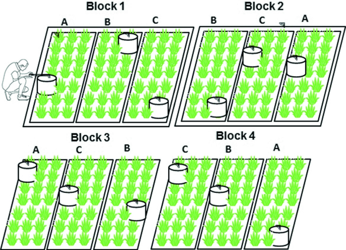

  

  A schematic diagram illustrating the collection of gas samples through a large chamber in a pineapple field

• Carefully insert the chamber base/frame using a wooden block and a hammer on the perimeter of each plot. Make sure that the metal trough of the chamber base is not damaged by forceful hammering. After insertion, the chamber base shall be levelled to the soil surface. Ensure that the base is not tilted to any side. This can be checked by pouring water into the trough of the base and observing the water level. If using a plastic chamber, then only the chamber without lid is inserted 2 weeks before measurements.

• In case of rice paddy or wetland (flooded condition), use a wooden boardwalk (above the water level) to reach the gas plots, to avoid soil compaction.

• Chambers should be insulated by wrapping appropriate insulating materials around them.

• Install a weather station at the field to collect data of rainfall, temperature, and moisture at different soil depths (e.g. 5, 10, 15, 20, and 30 cm).

• Prior to fertiliser application, composite soil samples from surface soil (preferably 0–10 cm) from each block shall be collected for basic physical and chemical analyses (texture, bulk density, soil pH, mineral N (NH₄⁺ and NO₃⁻), total N and total C. In addition, site information regarding latitude, longitude, altitude, soil type, previous, and current farm management practices, shall also be collected.

• Take extreme care by covering the chamber area during fertiliser application to the main field plot. After fertiliser is applied to main field plots, carefully remove the cover and apply the required amount of fertiliser to the area of each chamber.

• Test the linearity of gas fluxes from the given system in advance. Use 2–3 replicate chambers. After chamber deployment, sample headspace air at 0, 20, 40, 60, 80, 100, and 120 min after closing the chamber. Analyse the samples at the laboratory using a GC. In most cases, the gas emissions will be linear for at least 1.5 h. If yes, select the following times: 0, +30, and +60 min, or 0, +20, +40, and +60 for sampling from each chamber.

• Always perform the gas collection process at approximately the same time of the day, e.g. start roughly at 10 a.m. and finish at about 12. Record the temperature outside and inside the chamber at the time of gas sampling. After completing the gas sampling, remove chambers and store them in a suitable and safe place (dry, shaded, and cool).

• For each sampling event, ensure to record air and soil (7.5 cm) temperature using a thermometer, date, and amount of any rainfall or irrigation (mm), and soil moisture content (0–7.5 cm) on water-filled pore space basis (or take data from the datalogger if installed).

2.4.3 Gas and Soil Sampling

• Prepare syringes: label them consecutively (e.g. 1–24 depending on the total numbering of treatments) and additional syringes for air samples (labelled 01, 02, etc.).

• Make sure that the three-way tap or valve is properly connected to each syringe. Always hold the syringe by the three-way valve.

• Place all the syringes needed for each chamber next to the chamber.

• Aerate the chamber before placing it on the frame.

• Before placing the chamber on top of the base, fill the base frame with water using a watering can. The water in the enclosed space between the chamber and the base will act like a seal providing a barrier for gas diffusion. Make sure that enough water is in the gutter; be careful NOT to add any water anywhere else.

• Carefully place the chamber on the frame, make sure that it is sitting properly in the water-filled gutter.

• Connect the syringe to the three-way tap on the chamber (should be an air-tight connection).

• Open the three-way valves, pump 3–4 times and take the gas sample, and then close the three-way valve again.

• Immediately start the timer and leave it running for the entire sampling.

• Note down the date and time on the sampling sheet.

• Note down the air temperature in the chamber.

• Walk to the next chamber and place and repeat the above steps, work out a suitable time interval beforehand (e.g. 2–3 min), and maintain that same interval for the entire sampling period (Plate 2.15).

  Plate 2.15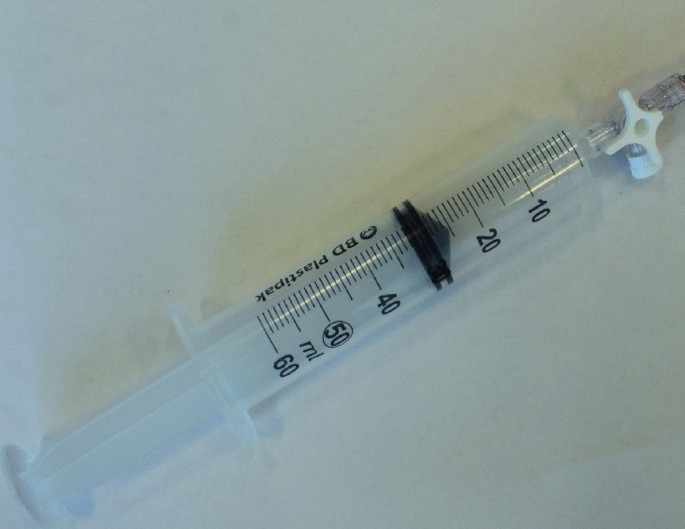

  

  Gas collection through a syringe in the field

• After a pre-defined cover period, take the second sample from the chamber. Get ready for the next sampling shortly before the sample time.

• In the case of many measuring plots, the second sample may need to be taken before the first round of samples is finished, which would require several people.

• If the sample containers are plastic syringes, gas samples must be analysed within 2 days (if the samples have not been transferred to a pre-evacuated exetainer). For longer storage, always store (and then analyse) calibration gases (gas standard) alongside the samples. Samples should always be pressurised (see above) with sample air (i.e. at least 20 ml in a 12 ml exetainer, ensuring that the overpressure can fill the sample loop if used). For further reading the paper of the Global Research Alliance by De Klein et al. (2020b) on safety measures is recommended.

• Perform gas flux measurements before treatment application to establish the baseline of each plot. Then take gas sampling immediately after fertilisation, other treatments, or extreme events (such as heavy rainfall). After fertiliser/manure/farm effluent application, measure every day for a week, then less frequently (3–5 days) at least once per week until the gas flux from fertiliser plots come to the background (control plot) level.

• To relate N₂O flux to N dynamics, collect soil samples in the surface layer (0–5 cm) to determine mineral N (NH₄⁺ and NO₃⁻ contents) throughout the entire experimental duration (more frequently shortly after the N application).

2.4.4 Safety Measures for GHG Sampling

• Nitrile gloves shall be worn during fieldwork.

• Extreme care should be taken while evacuating exetainer or transferring gas into exetainers to avoid any needle pricks (if not used to keep the needle in the protective cover).

• Tetanus injection record of staff involved in the field collection of gas samples should be up to date.

• Dispose of needles in a special container for needles.

• For GC operation, please refer to the relevant risk assessment and operating manual of the GC.

  For further reading the paper of the Global Research Alliance by de Klien et al. (2020b) on safety measures is recommended.

2.5 Calculation of GHG Fluxes

2.5.1 Overview

• 1. Analyse reference gases (i.e. gases that are available from commercial companies with a known concentration) using a GC to make a calibration curve (Fig. 2.5).

  Fig. 2.3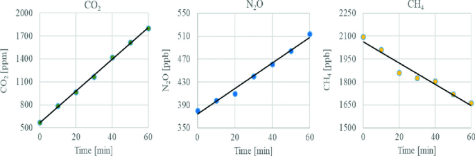

  

  Concentration of CO₂, N₂O and CH₄ in the headspace during the incubation

• 2. With the slope (a) of the regression line, calculate the gas concentration (y) of your samples (Eqs. 2.1 or 2.2). Gas concentration is usually given in ppm (10⁻⁶) or ppb (10⁻⁹).

• 3. Based on the concentration changes over time (Fig. 2.3), calculate gas fluxes according to Sect. 2.5.3

  Fig. 2.4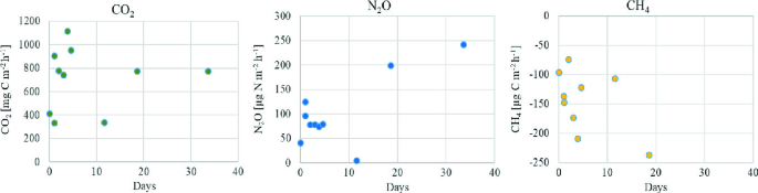

  

  Calculated emissions of CO₂, N₂O and CH₄ during a 35 day measuring campaign

• 4. In the last step of the calculation, convert gas concentration (ppm, ppb) to mass (mole or mg of gas, see Sect. 2.5.4). For each measurement you will get a separate flux (Fig. 2.4), the unit of the gas flux is usually ppm h^-1 or mg m^-2 h^-1.

2.5.2 Calibration

A calibration is a procedure to convert the GC output into a concentration unit, typically parts per million (ppm) or parts per billion (ppb). To develop a calibration curve (Fig. 2.5), normally three to four gas standards of known concentration are injected into a GC and analysed. Standard gas containing gas mixtures at increasing concentrations, contained in gas cylinders, can be ordered from commercial gas companies. With increasing gas concentrations, the GC output also increases. Either a linear increase (e.g. for CH₄) or a non-linear (CO₂ and N₂O) increase is observed which can be described by the following equations (Eqs. 2.1 and 2.2). Note, if the increase is linear, the term “a” in Eq. 2.2 is zero and the entire equation is reduced to a linear regression.

Fig. 2.5

Calibration with a linear (left) or quadratic (right) regression line

$$ {\text{Linear}}\,{\text{regression:}}\,{y} = {ax} + {b} $$

(2.1)

$$ {\text{Quadratic}}\,{\text{regression:}}\,{y} = {ax}^{2} + {bx} + {c} $$

(2.2)

where

x = area values (area of the standards, output from the GC),

y = % or ppm values (from the standards), and

a, b, c = regression parameters.

Steps of the regression analysis:

• The regression parameters for the appropriate equation suitable for the gas shall be copied into an excel spreadsheet beneath the calibration data.

• The process is carried out for all gases separately.

2.5.3 Calculation of the Gas Concentration and Fluxes

After all regression parameters are identified, the calculation of the concentration is, depending on the gas, carried out according to Eqs. 2.1 or 2.2.

From concentration to flux

The gas fluxes under a closed chamber are calculated for the duration of the gas sample collection. To do this, the concentrations are determined at several points in time (Fig. 2.6).

Fig. 2.6

Headspace-CO₂ concentration during the incubation and regression line for each plot. Green dots are flasks containing soil, blue is the control (containing water in the flask)

Based on the changes in concentration over time, the slope of the regression line at time = 0 is calculated (this corresponds to parameter “a” in Eq. 2.1 and parameter “b” in Eq. 2.2). Therefore, the slope of the regression line provides the flux rate as concentration/time. The unit of the flux rate is ppm h⁻¹.

Note, typically for N₂O and CO₂, we observe a positive slope, i.e. emission from soil to the atmosphere and for CH₄ under aerobic conditions the slope is negative, i.e. uptake of CH₄ by soil.

2.5.4 Conversion from Concentration to Mole

Transformation of concentration (ppm) in mole using the ideal gas law (Eq. 2.3):

$$ {n } = \frac{{{P} \cdot {V}}}{{{R} \cdot {T}}} $$

(2.3)

• where

• n = Number of moles of the examined gas

• P = Atmospheric pressure (Pa) [~100,000 = 1000 hPa] (to be measured)

• R = Gas constant (J mol⁻¹ K⁻¹) [8.314]

• T = Temperature (K) [273.15 + t °C] (t is the temperature to be measured)

• V = Volume of gas (i.e. N₂O, CO₂ or CH₄) in the chamber (m³). This is calculated by the multiplication of gas concentration with total chamber volume (V_tot) (ppm × 10⁻⁶ × V_tot).

Why do we convert gas concentration to its mass?

Gas concentration does not provide information about the total amount of gas measured or emitted. The smaller the chamber volume, the higher the concentration increases. Imagine a chamber volume of 1 m³ where gas concentration increases at 100 ppm h⁻¹. If the chamber volume is only 0.5 m³, this concentration increase would double up to 200 ppm h⁻¹.

Think: what would be the concentration change if the chamber volume would be 2 m³?

The answer is 50 ppm h⁻¹

Hence, to know the exact amount of a gas, in addition to the concentration (ppm or ppb), the volume and area of the chamber (V_tot, A), the atmospheric pressure (P, the higher the pressure the more gas molecules in the chamber), and the temperature (T, higher temperatures decrease the number of gas molecules per volume) must all be considered (see Eq. 2.3).

Example:

Temperature (T): 20 °C

Temperature: unit transformation °C to K: 20 + 273.15 = 293.15 K

Air pressure (P): 100,000 Pa

Chamber volume (V_tot): 0.02 m³

Chamber area (A): 0.1 m²

Concentration increase of the gas (CO₂) at t = 0 (ΔC): 1000 ppm CO₂ h⁻¹

Molecular weight of CO₂: 44.009 g mol⁻¹

Note, in the ideal gas law the Volume, V, refers to the gas we are interested in, i.e. CO₂, CH₄, N₂O. So, first of all the volume of this gas within the chamber volume, V_tot, is calculated:

V = V_tot * ΔC * 10⁻⁶ = 0.02 * 1000 * 10⁻⁶ = 0.00002 m³ h⁻¹

$$ \frac{\Delta n}{\Delta t} = \frac{{100,000{ x }0.00002 }}{{8.314{ x }293.15 }} = 0.00082\,{\text{mol}}\,{\text{CO}}_{2}\, {\text{h}}^{ - 1} $$

(2.4)

Multiplied with molar mass of CO₂ (44.009 g mol⁻¹), this corresponds to 0.03607 g CO₂ h⁻¹ or 0.00986 g CO₂–C (if only the active C component is applied with a molwt of 12.011 g mol⁻¹). This is now the emission rate from the plot the chamber has covered. To standardise the emission rate, we express it per m⁻²:

$$ F = \frac{0.00986 }{0.1 } = 0.0986\,{\text{g\,\,CO}}_{2}\!-\!{\text{C m}}^{ - 2}\, {\text{h}}^{ - 1} $$

(2.5)

The following information is required for flux calculation:

• Chamber volume (V_tot), which can be obtained by multiplying chamber length (L), width (W), and height (H) if it is a square-shaped chamber, for other shapes use the appropriate mathematical equation (or simply fill the chamber with water and measure the volume or weight of water…).

• Mole weight of the gas (as a rule, one converts to N₂O-N and CH₄/CO₂-C).

• Parameters of the gas law [temperature, atmospheric pressure, gas constant, covering time, and time of sampling during the cover period (t₀, t₁, t₂, etc.)].

Units and factors:

ppm: 10⁻⁶ or 1 μl L⁻¹

ppb: 10⁻⁹

ppt: 10⁻¹²

Molar masses:

CO₂: 44.009 g mol⁻¹

C: 12.011 g mol⁻¹

N₂O: 44.013 g mol⁻¹

N: 14.007 g mol⁻¹

CH₄: 16.043 g mol⁻¹.

For further reading the paper of the Global Research Alliance by Venterea et al. (2020) on flux calculation is recommended.

For further reading the papers of the Global Research Alliance by De Klein et al. (2020a) on data reporting and further calculations, by Dorich et al. (2020) on gap-filling techniques and by Giltrap et al. (2020) on modelling approaches are recommended.

2.5.5 Data Analysis

Data analysis is extremely important to produce realistic emission data. The most appropriate flux calculation method must be selected, and best interpolation of non-continuous measurements adopted to obtain best estimates of emissions and emission factors (EF) (Venterea et al. 2012) (Table 2.4). It is suggested that both gas analyses and data analysis, including appropriate statistical analysis, are performed in a laboratory equipped with staff familiar with all the required skills.

Table 2.4 Basic recommendations for GHG data analysis (adapted from Venterea et al. 2012)

A summary of GHG measurements, analysis, and data interpretation is presented in a schematic diagram below in Plate 2.16.

Plate 2.16

A schematic representation of gas sampling, analysis, and interpretation (© FAO/IAEA Mohammad Zaman)

2.6 Analysis of GHG Samples with Optical Gas Analysers

Gas chromatography is still the most widely used analytical technique for measuring GHGs from chambers (Plate 2.12a, b). It is a well-established, reliable, and robust method; the GC can also be linked to isotope-ratio mass spectrometers (IRMS) for analysis of the abundance of isotopes. In recent years, GCs have become more portable and automated, which makes it possible to run them unmanned in the field in connection with automated chambers. However, the greatest disadvantage of gas chromatography is that one can only measure discrete samples, and it takes several minutes to run a sample, which limits the number of gas samples that can be run (Rapson and Dacres 2014). These disadvantages can be overcome by employing optical gas analysers, which can conduct continuous gas measurements at a high temporal resolution (seconds to Hertz). The measurement principle of optical gas analysers utilises the ability of small molecules (e.g. H₂O, CO₂, CH₄, N₂O, and NH₃) to absorb infrared (IR) and near-infrared (NIR) light at unique wavelengths. Each molecule has a unique combination of atoms and, as a result, produces a unique IR spectrum when illuminated with IR light, which allows its identification. The light absorption at a specific wavelength, which is measured as light attenuation by a detector, is proportional to the concentration of a gaseous compound (Hensen et al. 2013; Rapson and Dacres 2014).

The general setup of an optical gas analyser consists of a light source from which light travels through the gas sample to an appropriate detector. The path that the light takes between the light source and the detector is called the optical path (Werle 2004). When the optical path lies directly in the outside air, it is called an open path system, whereas when the optical pass is enclosed inside a measurement cell (or cavity) where sample gas has to be pumped into, it is referred to as a closed path system (Hensen et al. 2013; Peltola et al. 2014). Depending on the specific optical technique utilised in an analyser, several mirrors and/or optical filters are added to the optical path to focus the light beam to increase light intensity and the length of the optical path. The main optical techniques employed for quantifying GHG are non-dispersive infrared spectroscopy (NDIR), Fourier-transform infrared spectroscopy (FTIR), photoacoustic spectroscopy (PAS), tunable laser absorption spectroscopy (TLAS), cavity ring-down spectroscopy (CRDS), and off-axis integrated cavity-output spectroscopy (OA-ICOS) (Werle 2004; Hensen et al. 2013; Peltola et al. 2014; Rapson and Dacres 2014).

NDIR and FTIR analysers use light sources that emit broadband IR radiation, e.g. IR lamps or black body light sources. In an NDIR analyser, broadband IR radiation passes unfiltered through the air sample. An optical filter in front of the detector determines which wavelengths are detected and thus which molecules are quantified. NDIR analysers are quite cheap and robust and often are used for quantifying CO₂ and H₂O in the air (Tohjima et al. 2009; Keronen et al. 2014). In FTIR analysers, the source radiation is constantly modulated by a set of mirrors called a Michelson interferometer containing different combinations of frequencies. For each combination, the amount of IR absorbed by the gas sample is measured. A Fourier transform is then applied to the raw data to calculate the absorption at each wavelength for the complete IR spectrum. This method allows the simultaneous quantification of many different gas species in air. Depending on the resolution of the FTIR analyser, it determines only gas concentrations (low-resolution FTIR) or isotopomers simultaneously (high-resolution FTIR) (Griffith et al. 2012; Rapson and Dacres 2014). In PAS, the light source is often a heated black body, but it can also be a laser. In contrast to NDIR and FTIR, PAS takes only indirect measurements of light absorption. The light passes through an optical filter to pre-select a specific wavelength, and a light chopper periodically “switches” the modulated light on and off before it is directed into the cavity via a mirror. Molecules heat up and expand when they absorb the modulated light, resulting in a pressure rise in the cavity. The light chopping creates pressure variations, which in turn generates acoustic signals that can be detected by microphones. The acoustic signals are proportional to the gas concentration of the target gas species (Iqbal et al. 2013; Rapson and Dacres 2014).

Analysers based on NDIR, FTIR, or PAS can operate with the measurement cell at ambient atmospheric pressure. This fact and the chosen light source reduce material costs and lead to lower prices in comparison to laser-based analysers utilising TLAS, CRDS, or OA-ICOS. Laser-based analysers do not operate with broadband IR radiation, but instead are tuned to the unique absorption line of a specific trace gas (Hensen et al. 2013). The cavity in such an analyser is kept at sub-ambient pressure, which results in narrower IR absorption lines and thus a higher gas species selectivity (Rapson and Dacres 2014). However, it also requires the analysers to be equipped with vacuum pumps and vacuum-proof tubing, tube fittings, and valves. The great advantage is that laser-based analysers are capable of fast and the most sensitive measurements of trace gas concentrations, as well as stable isotope compositions (including isotopomers) in the air (Hensen et al. 2013; Rapson and Dacres 2014; Brannon et al. 2016).

Nowadays, TLAS is the most common laser-based absorption technique for quantifying GHG concentrations in air. Commercially available analysers often employ either tunable diode laser absorption spectroscopy (TDLAS) or tunable infrared laser differential absorption spectroscopy (TILDAS) with quantum cascade lasers (QCL). Detailed information about these techniques is available in Li et al. (2013, 2014). The main disadvantage of TLAS is its susceptibility to instrument noise because the analysers rely on the measurement of a small change in light intensity against a large background light signal. To drastically improve sensitivity, TDLAS and TILDAS analysers are commonly equipped with multipass cells. In multipass cells, the light beam travels several times between aspherical mirrors before exiting the cavity in the direction of the detector, resulting in optical path lengths of several up to hundreds of metres. However, the mirrors are extremely sensitive to changes in alignment and, therefore, more sensitive to vibrations. This has led to the development of high-finesse optical cavities, which allow the build-up of large amounts of light energy in the cavity, boosting analyser sensitivity and robustness, but also decreasing cavity and analyser size. High-finesse optical cavities are the basis of CRDS and OA-ICOS (Rapson and Dacres 2014).

In OA-ICOS analysers, the laser beam enters the cavity at a non-zero angle so that the photons make thousands of passes between high-reflectivity mirrors before leaving the cavity again. This increases the effective optical path length to several thousand metres, enhancing the measured light absorption in comparison to multipass cells. The optical path length depends only on optical losses in the cavity, and therefore a precise laser beam alignment is not necessary, and the analysers are also less susceptible to slight changes in mirror alignments (Bakhirkin et al. 2004; Peltola et al. 2014; Rapson and Dacres 2014; Lebegue et al. 2016). In contrast, CRDS does not consider the absolute absorption intensity by the target gas species, but rather the rate of light intensity decay in the cavity. When the laser is turned on, the cavity is quickly filled with NIR light. As soon as a light intensity threshold is reached, the laser is abruptly turned off, and the light leaks out of the cavity with an exponential decay rate through the cavity mirrors. Additional light absorption in the cavity by the target gas species accelerates the light intensity decay rate, also known as ring-down time. The switching on and off of the laser takes place within microseconds, and the ring-down times are used to determine the concentrations of the target gas species in the cavity. Since the actual measurements take place when the laser is turned off, CRDS is not susceptible to laser intensity fluctuations or absolute laser power. The disadvantages, though, are that the mirrors have to stay very clean, and high-speed detection electronics are required (Rapson and Dacres 2014; Brannon et al. 2016). A laser-based optical technique, which has just been recently commercialised for GHG measurement, is laser dispersion spectroscopy (LDS). It tries to overcome the main limitation of TLAS, the detection of a small signal change against a large background, by measuring molecular dispersion instead of molecular absorption. The measurement signal is encoded in the light phase making the analyser more resilient to dirt and water vapour in the cavity because these compounds only affect light intensity (Nikodem and Wysocki 2012).

The past two decades have seen a rapid development of optical techniques and optical analysers for GHG measurements, and this trend is projected to continue over the coming years. One optical technique that might become more important is enhanced Raman spectroscopy (see Sects. 2.8.2 and 2.8.3). The range of commercially available optical gas analysers for different applications can be quite confusing; thus, Table 2.5 summarises the key points one should consider before purchasing a specific optical analyser.

Table 2.5 Key features of optical analysers

For a comparison of laser spectroscopic analyses of N₂O isotopomers, see Chap. 7, Sects. 7.3.4 and 7.3.5.

2.7 Hands-On Approaches Using a CRDS Analyser

2.7.1 Overview of the CRDS Techniques for Determining GHG Concentrations and Soil Fluxes

As outlined in Sect. 2.6 (“Analysis of GHG samples with optical gas analysers”), the advent of laser-based techniques has enabled real-time measurement of soil gas fluxes in the field. In recent years, CRDS has become of particular interest to researchers due to its ability to measure GHG concentrations with a very high precision in field settings. For example, the Picarro G2508 multi-species gas analyser allows CO₂, CH₄, N₂O, NH₃, and H₂O to be measured simultaneously. CRDS analysers have three key advantages for soil gas flux measurements in comparison to traditional GC measurements: (1) it enables the detection and measurement of low levels of GHG fluxes. Areas with low emission rates, while not significant in the short-term, may be of great interest to calculate the global GHG budget when extrapolated over longer timescales and large surface areas; (2) multi-species measurements allow for direct correlations between gas species. The processes and sources associated with the emission (or uptake) of GHGs may require more than one axis for proper characterisation; and (3) the high sampling frequency of real-time measurements leads to a better characterisation of soil flux profiles and shorter closure times for soil flux chambers. In addition, the real-time nature of this system provides instant feedback on site selection and omits sampling and storage effects.

The sub-section below describes the fundamentals of CRDS and discusses how a CRDS analyser may be paired with commercial and home-made closed chambers to create a field and/or laboratory deployable flux system.

2.7.2 Theory: Near-Infrared Absorption Spectroscopy Fundamentals

Nearly every small gas-phase molecule (e.g. H₂O, CO₂, CH₄, N₂O, etc.) has a unique near-infrared absorption spectrum, and this is generally also true for different isotopologues (¹²CO₂ vs. ¹³CO₂, ¹²CH₄ vs. ¹³CH_4, etc.) (for details, see Chap. 7). At atmospheric pressure, these spectra are very broad and continuous, but at sub-atmospheric pressure the contributions from individual vibrational modes are well resolved so that each spectrum is made up of distinct absorption lines; each line is centred at a characteristic wavelength and possesses an extremely predictable line shape. Under these conditions, it is generally possible to find one or more narrow wavelength frequency ranges where the target molecule has strong absorbance features, and the absorbance contributions from other molecules are minimal. Therefore, the spectrum for each molecular species can be thought of as a unique and very information-rich “fingerprint”.

After choosing a specific wavelength range, the concentration of the target gas can be measured by determining light absorption. In principle, the concentration could be inferred from the light loss at the absorbance maximum of the target gas; however, in practice, it is far more useful to scan over a specific absorption line by using a tunable, narrow-band laser to measure absorption in small steps over the relevant frequency range. The main advantage of determining the full spectrum of an absorption line is that one can measure multiple gases at the same time and that it also allows to measure the background level of light absorbance in one step. A measured absorption spectrum s can then be described as the weighted sum of contributions from individual gases and from the background light loss (Fig. 2.7) and (Eq. 2.6).

Fig. 2.7

An example spectrum “s” (top left) is the sum of background light loss “b”, and scaled gas-specific absorbance spectra “g1” and “g2” (bottom). In this fictional example, ${s} = {b} + 1000 \times { g}_{1} + 500 \times {g}_{2}$

$$ {s} = {b} + {a}_{1} {c}_{1} {g}_{1} + {a}_{2} {c}_{n} {g}_{n} $$

(2.6)

where b is the background light loss, g is the spectrum specific for each gas, a is a scaling factor describing the fundamental absorbance strength of the gas, and c is the scaling factor the concentration of each individual gas molecule. If the values of b, a, and g are known, then the gas concentrations c can be determined from the observed spectrum s. Since a and g are fundamental properties of the respective gas, they can be established in advance. The background light loss b is specific for each instrument but is generally highly stable over time.

2.7.3 Operational Principle of Cavity Ring-Down Spectroscopy

Cavity ring-down spectroscopy allows the concentration and isotopic composition of gases to be measured with very high precision. A key feature of CRDS is that it measures the decay of light in the measurement cell instead of measuring absolute absorption intensities, where the term “ring down” in CRDS is referring to this principle of measuring the light loss in the cavity over time. The cavity itself consists of three high reflectivity mirrors, and the light from a continuous-wave, single-frequency tunable laser diode is reflected between the mirrors (Fig. 2.8). When the laser is turned on, the cavity quickly fills with the circulating laser light. Because the mirrors have slightly less than 100% reflectivity (99.999%), a small amount of light continuously leaks out and is measured with the photodetector. As soon as the light intensity reaches a threshold (within a few tens of microseconds), the laser is abruptly turned off, and the light already within the cavity bounces between the mirrors (about 100,000 times). As the light circulates between the mirrors, light is absorbed by the target gas in the cavity, and the photodetector measures the exponential decay curve, also known as ring downs. In the absence of the absorbing gas, the decay rate is determined solely by the reflectivity of the mirrors.

Fig. 2.8

High finesse optical cavity with a three-mirror configuration. Top: no absorbing species in the cavity = long ring-down time. Bottom: absorbing species present in the cavity = short ring-down time

The ring downs are measured in real time by the photodetector, and the exponential decay curve consists of several thousand individual light measurements. A dedicated signal processor fits this curve to determine the decay rate. To obtain a spectrum, the laser frequency is tuned over a sequence of narrow frequencies, and the ring-down rate is measured for each step (Fig. 2.9). Once a spectrum is obtained, algorithms are used to recover the spectrum contributions from each gas and from background light loss processes, as previously described. Critically, the decay rates are independent of the initial laser light intensity, and as such, the measurement is not affected by laser intensity fluctuations or absolute laser power.

Fig. 2.9

The laser frequency is stepped, and a ring-down measurement is made at each step, generating a series of exponential decay curves (left). The software fits each curve to discover its decay coefficient. Representing these coefficients as absorbance, we obtain an absorbance spectrum (right). Numbers indicate corresponding decay curves and absorbance spectrum data

2.7.4 Minimum Detectable Flux (MDF)

CRDS analysers allow GHG concentrations to be measured with a higher frequency and precision than generally possible with GC techniques. These key advantages allow either to determine GHG fluxes with a higher precision or to achieve the same level of precision within a shorter amount of time. The latter is of importance because a reduction in enclosure time minimises negative effects resulting from the use of a closed static chamber.

Christiansen et al. (2015) investigated the relationship between enclosure time and instrument precision and introduced the concept of minimum detectable flux (MDF) to determine the lower limit of flux rates that can be achieved with a given measurement precision (Eq. 2.7):

$$ {\text{MDF}} = \left( {\frac{{A_{\text{A}} }}{{t_{\text{c}} }}} \right)\left( {\frac{V P}{A R T}} \right) $$

(2.7)

where A_A is the analytical precision in ppm, t_c is the closure time of the chamber in hours, V is the chamber volume in L, P is the atmospheric pressure in Pa, A is the chamber area in m², R is the gas constant in L K⁻¹ mol⁻¹, and T is the ambient temperature in K. The equation describes that the MDF can be reduced by either increasing the enclosure time or by increasing the analytical precision (reducing the analytical uncertainty).

Nickerson (2016) highlighted the practical importance of the increased measurement frequency of CRDS analysers since an increase in measurement number n will reduce the standard error A_SE compared to the raw precision A_A of the CRDS analyser (as A_SE = A_a/$\surd{n}$). Therefore, he suggested that the effective MDF should consider the measurement/sampling frequency (Eq. 2.8):

$$ {\text{MDF}} = \left( {\frac{{A_{\text{A}} }}{{t_{\text{c}} \surd \frac{{t_{\text{c}} }}{{p_{\text{s}} }}}}} \right)\left( {\frac{V P}{A R T}} \right) $$

(2.8)

where p_s is the sampling periodicity in hours. For a CRDS analyser, the sampling periodicity is about every 8 s. The GC measurements are based on discrete samples, and the sampling frequency can vary significantly based on the research focus, but typically samples are taken every 5–15 min. Consequently, real-time CRDS analysers achieve a higher precision for a flux estimate than GC measurements, given the same chamber system, deployment time, and assuming a similar raw precision for the two techniques (Fig. 2.10). Or in other words, a prescribed MDF can be achieved within a shorter amount of time with CRDS compared to GC measurements.

Fig. 2.10

(figure adapted from Nickerson 2016)

Effect of sampling/measurement frequency on the time needed to reach a certain CH₄ minimum detectable flux (MDF). Real-time CRDS analysers report a concentration measurement about every 8 s, while discrete sampling for GC measurements commonly occurs every 5–15 min (i.e. 300–900 s). Due to the higher integration time, the CRDS analyser achieves a prescribed MDF within a shorter amount of time (an MDF of 0.1 µmol CH₄ m⁻² h⁻¹ is reached within 700 s with CRDS and within about 2300 s for 5 min interval GC sampling). The illustration assumes that the CRDS and GC measurements show the same raw precision. MDF was calculated on the following parameters: A_a = 0.01 ppm, V = 0.5 m³, P = 101325 Pa, A = 1 m², R = 8.31448 J K⁻¹ mol⁻¹, and T = 295 K

2.7.5 Selecting the Appropriate Flow Path

CRDS analysers have a continuous flow-through design that pulls gas through the analyser at a fixed flow rate (typical flow rate for a concentration CRDS analyser is ~250 ml min⁻¹). Automated pressure control loops within the analyser can be adjusted to gradual changes in input pressure and flow, but under normal operation, gas enters and leaves the analyser at the same flow rate. This design characteristic makes it suitable for use in recirculation experiments. Depending on the chamber design, the CRDS analyser can act as the primary source of flow or as a secondary sampling source, referred to as in-line or parallel, respectively.

2.7.6 In-Line Flow Path

In this setup, the CRDS analyser is typically the primary source and control of flow in the recirculation setup (Fig. 2.11). It is commonly used with custom-made chambers or commercial chambers that do not employ their own flow control. When designing such a setup, users need to be mindful of any restrictions or rapid changes of flow that may occur during measurement. Inlet tubing length should not exceed 15 m and should have appropriate filtration in place to protect the analyser from dust and liquid water (see the next section). The CRDS analyser acts as the primary data repository for concentration and external sensor data (chamber temperature and pressure) and can control and coordinate chamber operation (if available).

Fig. 2.11

Flow path of an in-line arrangement with a CRDS analyser in combination with a recirculation pump and a soil chamber. Additional communication or control cables are not shown

2.7.7 Parallel Flow Path

The parallel flow arrangement is typically used when the analyser acts as a complementary or additional instrument in an existing recirculation setup. The user may have an existing flow setup that is controlled by a primary pump, or they may be using an existing chamber-analyser system (e.g. LI-COR LI-8100A, for details, see Chap. 3, Sect. 3.2.2). Since the CRDS analyser is no longer the primary source of flow control, it is essential that the flow rate of the main recirculation setup is higher than that of the CRDS analyser. The greater the difference between the two, the smaller the influence of the CRDS analyser will be.

2.7.8 Multiple Chambers

It should be noted that many commercial and homemade chambers often come with multiplexers–the ability to deploy and connect multiple chambers to a single analyser. A CRDS analyser can be used with a multiplexer in both the in-line or parallel arrangements.

The connection location of the CRDS analyser should follow the same approach as shown in Figs. 2.12 and 2.13. In either case, the multiplexer is located in the place of the chamber.

Fig. 2.12

Flow path of a parallel arrangement with a CRDS analyser, a recirculation pump, and a mobile soil gas survey system (LI-COR LI-8100A). Additional communication and control cables are not shown. Note the higher flow rate of the main recirculation setup at 1000 ml min⁻¹, and the parallel connection of the CRDS inlet and return on the return flow of the LI-COR analyser

Fig. 2.13

Flow path for a multiple chamber setup. Deployments with multiple chambers are popular when a large surface area is to be monitored over a long period of time

2.7.9 Calibration

The concentration readings of a CRDS analyser behave very stable over time, and therefore, it is not necessary to calibrate the concentrations daily or weekly. However, it is advisable to check the accuracy and performance of a CRDS analyser on a monthly to yearly basis. This can be done by measuring standards from compressed gas cylinders. The concentrations measured by the CRDS analyser are then compared to the accepted value of the gas cylinder. The quality/accuracy of the final analyser calibration reflects (1) the number of standards, (2) the compositional range of the standards, (3) the method of standard measurement, and (4) the accuracy and precision of the standard itself:

• 1. The minimum number of different standards to calibrate the slope and offset of the analyser is two, and because CRDS instruments are highly linear, this is often enough. However, it is recommended to measure at least three or more standards, to confirm both the linearity of the instrument and the quality of the standards.

• 2. The range of the standards should generally encompass or exceed the expected concentration range of the sample air and should fall within the guaranteed specification range of the analyser.

• 3. The gas cylinders can either be connected directly to the CRDS analyser or the gas can be introduced via a gas bag (e.g. Tedlar bag). Direct connections to a tank are preferred as they minimise the chance of leaks and eliminate any dilution of the standard from remnant gas in the bag. Tedlar bags are an acceptable option, but they may lead to a lower degree of confidence in calibration. For applications where 1–10 ppm levels of accuracy are required, a direct connection to a tank is recommended.

• 4. It is commonly accepted that primary standards, when compared to secondary or even tertiary standards, have higher levels of accuracy. Having confidence in the value of the standards leads to a higher degree of confidence in the calibration of the instrument. It is advisable to assess whether the accuracy and precision of the standards are high enough for the research needs.

2.7.10 Advanced Application Considerations: Filtration of Gas Samples

The precision of an absorption measurement within a CRDS analyser can degrade under the presence of foreign particles that scatter or absorb light. To overcome this potential issue, the inlet of a CRDS analyser is generally equipped with two 4 nm particulate filters. One is user-replaceable, and the other can only be replaced in a cleanroom environment. To prevent long-term damage to the sample handling of the analyser and maintain a healthy cavity, external filters are recommended.

Of primary concern are particles that can potentially be pulled into the sample handling of the analyser via the inlet port. In order to select and build a proper filtration system, the user must first assess which, if any, particles are potentially present in the field. Arid environments with high wind speeds or other mechanical means of increasing particle load (walking, driving, animals, etc.) pose a much greater danger to the analyser than vegetated surfaces. In most cases, a cheap, user-replaceable Acrodisc^®, 0.2–1 µm is enough to remove most particles. The frequency of replacement should be dictated by the particle load of the gas sample and the flow rate through the filter.

2.7.11 Liquid Water and Water Vapour

One of the biggest risks to any field-based system is exposure to liquid water. In this section, we focus on the introduction of liquid water through the inlet of the analyser as a result of (1) condensation or (2) actual sampling of liquid water (precipitation, ground saturation, etc.).

Long-term deployments of CRDS analysers can subject them to environments with temperature variations that exceed the operating range of the system (10–35 °C). Custom or commercially available enclosures are used to provide a measure of temperature control and/or protection from the elements (rain, snow, wind, etc.). The temperature difference between the exterior and interior of the enclosure can lead to condensation in sampling lines. This problem is particularly evident in scenarios where hot and humid gas is brought into a cold enclosure. To reduce the likelihood of condensation, desiccants such as Drierite or magnesium perchlorate can be used to reduce the water vapour level in the sample gas. Such desiccants are also practical if water vapors need to be reduced below 4 vol%, the operational limit for a CRDS analyser.

If condensation, or the presence of liquid water through direct sampling, cannot be avoided, then a water trap must be used before the inlet of the analyser. The volume of a water trap should be appropriate to handle any input of liquid water. It is also possible to install water traps with automatic draining capability so that the system may operate in a user-free fashion. It is important to note that a water trap will add additional volume to the recirculation system, something that needs to be considered when flux calculations are performed.

2.7.12 CRDS-Specific Considerations

A CRDS analyser is a laser absorption spectrometer. Under specific conditions, the composition of the sample gas may have unintended effects on the spectra. If levels of ethane, ethylene, acetylene, or hydrogen sulphide exceed atmospheric levels, the user should consult manufacturer documentation to determine the effects of these species on their measurements of greenhouse gases. In many cases, the installation of an additional scrubber may be used to remove an interfering species. One such example is the removal of hydrogen sulphide using laboratory-grade copper filings (Malowany et al. 2015). Figure 2.14 illustrates how a recirculation setup can be adjusted for specific field conditions by adding a particulate filter, a water trap, and a copper scrubber.

Fig. 2.14

Example setup of a CRDS analyser for field deployment in a forest environment. The copper scrubber is in place as trace amounts of H₂S are expected, the water trap is used to minimise the change of liquid water entering the system due to ground saturation during long rainfall events, and the particulate filter is there to prevent particles that may enter the air stream. Not shown on this image is an enclosure for the system and a stable supply of power

The composition of the carrier gas, specifically any significant changes to the N₂–O₂ ratio of the carrier gas, will have pressure broadening effects on the spectra (Nara et al. 2012). This can result in a degradation of accuracy. The installation of an additional oxygen sensor inside a CRDS analyser, or any external oxygen sensor, can help the user detect changes in the N₂–O₂ ratio and apply a correction. The manufacturer also offers a pre-configured mode for pure N₂ carrier gases. It should be noted that major changes to Argon (Ar) or Helium (He) will have the same effects. More importantly, a pure He carrier can permanently damage a CRDS analyser.

2.7.13 Datalogging and Flux Processing

All concentration data obtained using a CRDS analyser is automatically stored on the hard drive of the analyser. This raw data can then be processed using the CRDS software or other, third-party compatible software that is usually supplied by the chamber manufacturer to obtain flux values. In order to convert concentrations into fluxes, the software will ask the user to enter the chamber and tubing volume, chamber surface area, chamber and soil temperature, and chamber pressure. Depending on the software package used, it may be possible to monitor the accumulation of the gases in real time or apply post-processing using three or more fitting algorithms: linear (Eq. 2.9), quadratic (Eq. 2.10) (Wagner et al. 1997), or Hutchinson and Mosier (1981) (Eq. 2.11).

Linear:

$$ {y} = {\text{slope}} \times {X} + {\text{background}} $$

(2.9)

Quadratic:

$$ {y} = {\text{a}} \times {X}^{2} + {\text{slope}} \times {X} + {\text{background}} $$

(2.10)

Hutchinson and Mosier:

$$ {y} = {\text{background}} + {\text{step}}\left( {1 - {\text{e}}^{{ - {\text{slope}} \times {X}/{\text{step}}}} } \right) $$

(2.11)

Custom fitting options are available in certain software packages (Fig. 2.15).

Fig. 2.15

Example of a Hutchinson and Mosier fitting algorithm applied to a measurement of H₂O on a CRDS analyser

CRDS analysers are compatible with the streaming of data to external datalogger using RS232, Ethernet, or analogue communication protocols. In addition, it is also possible to incorporate external sensor data such as pressure and temperature probes within the soil flux chamber. Detailed support and integration documentation are available from the manufacturer.

2.8 Enhanced Raman Spectroscopy of Greenhouse Gases

Enhanced Raman spectroscopy emerged in recent years as a powerful analytical tool for highly selective identification and simultaneous quantification of multiple components in complex gas mixtures (Hanf et al. 2014; Frosch et al. 2013a; Jochum et al. 2015a; Hippler 2015; Kiefer 2015; Knebl et al. 2017). Conventional Raman spectroscopy was already discovered in the 1920th (Long 2002; Smekal 1923; Raman and Krishnan 1928; Landsberg and Mandelstam 1928; Kramers and Heisenberg 1925), but its application in real-world applications was very limited until recently, due to the inherently weak signal intensities and technical limitations.

2.8.1 Raman Spectroscopy of Gases

Raman spectroscopy is based on inelastic scattering of light. When monochromatic laser light is guided through a gas sample, most photons pass the analyte volume without any interaction and thus provide no gas specific chemical information. The scattering cross section σ is only around 10⁻²⁷ cm² for typical gases. Thus, only a small fraction of the photons is scattered by the gas molecules which also have a very low number density. The major part of the scattered radiation results from elastic scattering (Rayleigh scattering) and has the same frequency as the excitation light. Inelastic scattering occurs with approximately three orders of magnitude smaller intensity. The frequency shift of the inelastically scattered light is caused by the energy transfer in the rotational, vibrational, or rotational–vibrational states of the molecules and is thus the basis of the unique chemical selectivity of Raman spectroscopy. Raman scattering and the more established IR absorption are complementary effects that probe molecular vibrations and rotations. Raman scattering depends on the changes in the polarisability of the molecule during the rotation/vibration, while IR absorption relies on changes in the (permanent) dipole moment. Thus, IR absorption spectroscopy is not sensitive to diatomic homonuclear molecules such as oxygen (O₂), hydrogen (H₂), or nitrogen (N₂) which provide no permanent dipole moment for light interaction. In contrast, inelastic Raman scattering does not require a permanent dipole moment of the molecules, and the specific molecular transitions must not be matched with the excitation wavelength. Thus, Raman spectroscopy is a powerful method for the analysis of all but noble gases with only one monochromatic laser source. A whole suite of biogenic gases, including CO₂, N₂O, O₂, CH₄, H₂, and N₂, can be identified and quantified simultaneously (Fig. 2.16).

Fig. 2.16

Reprinted with permission from Hanf et al. (2015a). Copyright 2015 American Chemical Society

Raman spectrum of the rotational and rovibrational bands of a complex mixture of biogenic gases, including CO₂, N₂O, O₂, CH₄, H₂, and N₂.

2.8.2 Enhanced Raman Gas Spectroscopy

Conventional Raman spectroscopy is an extremely weak process. Recent advances in laser as well as detector technology, new highly efficient optical filters, and optical components develop Raman spectroscopy into a comprehensive technique for multigas analysis. The Raman Stokes intensity $I_{\text{R}}$ depends on the laser intensity $I_{0}$, the angular frequencies of the laser $\omega_{\text{L}}$ and the scattered light $\omega_{\text{R}}$ as well as the polarisability $\alpha$ of the molecule, and the number $N$ of molecules of the measured gas (Eq.  2.12).

$$ I_{\text{R}} = {\text{const}}*N* I_{0} *\left( {\omega_{\text{L}} - \omega_{\text{R}} } \right)^{4} *\left| \alpha \right|^{2} $$

(2.12)

The originally small inelastic scattering signals of the gas molecules must be increased with the development of enhancement techniques based on the above-given parameters in order to achieve high sensitivities. Raman gas sensors are nowadays based on specific multi-pass cavities, high-pressure cells, or the application of high-power lasers (Li et al. 2008; Kiefer et al. 2008; Schiel and Richter 1987). Two very promising techniques, which were recently developed, are fibre-enhanced Raman spectroscopy (FERS) (Hanf et al.2014; Knebl et al. 2018) and cavity-enhanced Raman spectroscopy (CERS) (Frosch et al 2013a).

In FERS, the number N of gas molecules that contribute to the Raman signal (Eq. 2.10) is extremely increased. In conventional Raman spectroscopy, the signal is excited and collected from a small scattering volume (Fig. 2.17a) (Frosch et al. 2013b). This limitation can be overcome with the help of hollow-core optical sensor fibres. In elaborated micro-structured hollow-core optical fibres, the light can be guided with extremely low attenuation within a certain spectral range (Russell 2003; Knight 2003; Hartung et al. 2015; Yan et al. 2017a, b). By filling the gas in the same inner hollow core of the fibre, light and analyte are both guided in the same volume and thus the analyte is efficiently excited over an extended path length (Fig. 2.17b) and the number of scattering molecules is strongly increased (Frosch et al. 2013b). In other words, the Raman fibre sensor can be seen as optimised cuvette and provides strongly enhanced analytical sensitivity (Hanf et al. 2014; Frosch et al. 2013b; Knebl et al. 2019; Jochum et al. 2016; Hanf et al. 2015a; Boegoezi et al. 2015; Sieburg et al. 2019). A highly efficient FERS setup was developed for gas analysis (Figs. 2.17 and 2.18).

Fig. 2.17

Reprinted with permission from Frosch et al. (2013b). Copyright 2013 American Chemical Society

Comparison of conventional Raman spectroscopy (a) and fibre-enhanced Raman spectroscopy (b). Conventional Raman setups suffer from the limited interaction volume of excitation light and analyte gas (a). In FERS, the excitation light is guided over an extended range within the hollow core of the optical fibre, which also functions as minimised analyte container (b). An excellent light–analyte interaction is achieved in fibre-enhanced Raman spectroscopy and a high number of molecules contribute to the Raman signal (Frosch et al. 2013b).

Fig. 2.18

Reprinted with permission from Hanf et al. (2014). Copyright 2014 American Chemical Society

Design of the optical setup for fibre-enhanced Raman spectroscopy (FERS) (Hanf et al. 2014) consisting of Laser, telescope (T), long-pass dichroic beam splitter (DC), objective lens (OL), fibre adapter assembly (A1 and A2), hollow-core photonic crystal fibre (PCF), power metre (PM), pinhole (P), edge filter (E), aspheric lens (L), spectrometer (SPEC), and CCD detector.

In CERS, the weak inelastic scattering signals of the gas molecules can be increased by up to six orders of magnitude with the help of a high finesse optical cavity. One of the developed gas sensors consists of a miniaturised laser diode with λ_exc. = 650 nm (Frosch et al. 2013a; Keiner et al. 2013, 2014) which is passively frequency locked and feedback coupled to a high finesse cavity, enabling a power build-up to 100 W (Frosch et al. 2013a). The cavity components are aligned for spatial mode matching of the input beam and the Gaussian beam supported by the power build-up cavity (PBC), while the facet of the laser diode helps in stabilising mode matching by spatial filtering (Frosch et al. 2013a). Such arrangement of the PCB is extremely stable to mechanical vibrations (Frosch et al. 2013a), and it has been shown that concentration fluctuations of about 50–100 ppm can be monitored within measurement times of one second (Frosch et al. 2013a).

Main advantages of enhanced Raman spectroscopic gas sensing include the following:

• All gases, except noble gases, can be analysed, including diatomic homonuclear molecules such as oxygen (O₂), hydrogen (H₂), and nitrogen (N₂).

• A whole suite of gases can be identified simultaneously (Fig. 2.16) with no cross sensitivities and the use of only one excitation laser.

• A priori unexpected gases can easily be identified in the Raman spectra of complex multigas compositions, in contrast to simple gas sensors that must be designed for all expected gases beforehand.

• As direct spectroscopic method, which is based on the intrinsic molecular vibrations, Raman gas sensing does not need any labels or transducers and does not suffer from saturation, bleeding, poisoning, etc. This optical technique does not need direct physical contact with the analyte gas. Measurements can be performed through an optical window and remote.

• The technique is non-consumptive. The gas concentrations are not disturbed due to the measurement process, and small gas exchange processes can be monitored continuously online in closed cycle experiments.

• The Raman scattering intensity offers perfect linearity with the analyte concentration (Eq. 2.10) and allows for robust instrument calibration over a broad concentration range from ppm to pure compounds. Trace gases can be quantified on the background of a higher concentrated gas matrix.

• The fast Raman spectroscopic measurement enables online monitoring of temporal changes in gas concentrations during process.

• Stable gas isotopes can be distinguished (due to changes in the reduced mass and thus spectral position, see Fig. 2.19) and be used as tracers to follow specific pathways.

  Fig. 2.19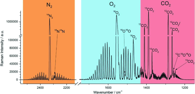

  

  Adapted with permission from Knebl et al. (2019). Copyright 2019 American Chemical Society

  Combined Raman spectra containing the rovibrational bands of ¹⁴N₂, ¹⁴N¹⁵N, ¹⁶O₂, ¹⁸O¹⁶O, ¹⁸O₂, ¹⁶O₂, ¹²C¹⁶O₂, ¹³C¹⁶O₂, and ¹²C¹⁸O¹⁶O.

• Raman devices can be highly miniaturised for field deployment.

2.8.3 Enhanced Raman Spectroscopic Analysis of Greenhouse Gases

Research regarding enhanced Raman spectroscopy of biogenic gases can be divided into three areas: (i) The capability for unambiguous identification and quantification of various gas mixture components to follow the formation, spread, and exchange as well as storage of gases (Frosch et al. 2013a; Jochum et al. 2015a, b; Keiner et al. 2013, 2014, 2015a, b; Sieburg et al. 2017, 2019; Hanf et al. 2015b). One focus is the analysis of the respiratory quotient (RQ, CO₂ released per O₂ consumed during respiration) as an indicator of changes in substrate use and metabolism (Jochum et al. 2015a; Keiner et al. 2013; Sieburg et al. 2017; Hanf et al. 2015b); (ii) the monitoring of stable isotopes (^12/13CO₂, ^14/15N₂, ^14/15N₂O, and ^16/18O₂) alongside unlabeled gases as tracers for specific pathways (Knebl et al. 2019; Keiner et al. 2014, 2015a, b); and (iii) the unique ability for direct quantification of nitrogen at natural background to study pathways of the nitrogen cycle (e.g. denitrification, N₂ fixation) (Keiner et al. 2015a; Kumar et al. 2018; Jochum et al. 2017).

The RQ value was analysed as an indicator of changes in plant metabolism under drought stress (Fig. 2.20) (Hanf et al. 2015b). It was discovered that pine (Pinus sylvestris) can switch from carbohydrate-dominated respiration to a mixture of substrates during several days of drought stress, but spruce (Picea abies) cannot (Hanf et al. 2015b). The onsite analysis of depth profiles of soil gases in the Hainich critical zone exploratory showed that the concentrations of O₂ and CO₂ were largely decoupled, and complex processes in previously uncharacterised environments can be studied (Sieburg et al. 2017). The ability to monitor the inert tracer sulphur hexafluoride (SF₆) alongside biogenic gases under consideration allows for thorough online gas leakage correction to avoid under- or overestimation of biological activity such as respiration or photosynthesis (Fig. 2.21) (Jochum et al. 2015b).

Fig. 2.20

Adapted with permission from (Hanf et al. 2015b). Copyright 2015 Royal Society of Chemistry

Example for monitoring dark respiration rates of a branch of untreated pine. The individual respiration rates (both O₂ and CO₂) are used to calculate subsequent RQ values (Hanf et al. 2015b).

Fig. 2.21

Adapted with permission from Jochum et al. (2015b). Copyright 2015 American Chemical Society

Example of an experimentally acquired multigas Raman spectrum, consisting of the biogenic gases O₂, CO₂, N₂, H₂, CH₄, and the tracer gas SF₆.

The discriminatory power of Raman spectroscopy was used to monitor several stable gas isotopes simultaneously to investigate the labelling of young poplar trees under aphid infestation with ¹³CO₂ to analyse the possible incorporation of ¹³C in defense compounds (Keiner et al. 2014, 2015b). A combination of ¹³C-labelling and RQ analysis was applied to investigate the microbial degradation of ¹³C-labelled benzene in soil against the background of the heterotrophic soil respiration (Jochum et al. 2015a). By combining ¹³CO₂ and ¹²CO₂ as well as ¹⁸O₂ and ¹⁶O₂ measurements in one setup, it was proposed to use carbon dioxide and oxygen isotopologues to track and disentangle different overlaying processes and to help elucidating the contributions of photosynthesis, photorespiration, and respiration to the net gas exchange of plants (Knebl et al. 2019).

The nitrogen evolution was continuously monitored over the stepwise enzymatic denitrification of labelled and unlabeled nitrate by Pseudomonas stutzeri (Fig. 2.22) (Keiner et al. 2015a). The simultaneous quantification of the whole gas phase also enabled the contactless and sterile online acquisition of the pH changes in the P. stutzeri culture by the stoichiometry of the redox reactions during denitrification and the CO₂-bicarbonate equilibrium. Continuous pH-monitoring–without the need to insert an electrode into a sterile solution–elucidated an increase in the slope of the pH value coinciding with an accumulation of nitrite, which in turn led to a temporary accumulation of N₂O, due to an inhibition of N₂O reductase (Keiner et al. 2015a). The gas quantification was complemented with the analysis of nitrate and nitrite concentrations for the online monitoring of the total nitrogen element budget (Fig. 2.23) (Keiner et al. 2015a). In an investigation of the thiosulfate- and hydrogen-driven autotrophic denitrification by a microbial consortium enriched from groundwater of an oligotrophic limestone aquifer, the turnover reactions of electron donors (thiosulfate and H₂) were traced, as well as electron acceptor (nitrate), gaseous intermediates, and end products (¹⁵N₂, ¹⁵N₂O, CO₂, H₂, ¹⁴N₂, and O₂) in the headspace, using Raman gas spectroscopy (Kumar et al. 2018). N₂ production and H₂ consumption rates were calculated under denitrifying conditions and followed the electron donor usage of the bacterial consortium. Recently, the biological nitrogen fixation of a Medicago sativa–Rhizobium consortium was, for the first time, directly investigated at natural background and without a proxy or isotopic labelling, by continuously analysing the amount of atmospheric N₂ in static environmental chambers (Jochum et al. 2017).

Fig. 2.22

Adapted with permission from Keiner et al. (2015a). Copyright 2015 Elsevier

Raman spectroscopic multigas monitoring of the denitrification of ¹⁵N-nitrate by Pseudomonas stutzeri (Keiner et al. 2015a). The concentration courses of ¹⁵N₂, CO₂, ¹⁵N₂O, and the calculated pH value are shown as well as the sum of the nitrogen gases ¹⁵N₂ + ¹⁵N₂O.

Fig. 2.23

Adapted with permission from Keiner et al. (2015a). Copyright 2015 Elsevier

Concentration courses of nitrate, nitrite, nitrous oxide, and dinitrogen during the successive reduction ${\text{NO}}{_{3}}^{ - } \to {\text{NO}}{_{2}}^{ - } \to {\text{NO}} \to {\text{N}}{_{2}} {\text{O}} \to {\text{N}}_{2}$ (Keiner et al. 2015a). Continuous Raman gas concentrations of ¹⁵N₂, ¹⁵N₂O, and CO₂ are represented by solid lines. The total nitrogen balance from all nitrogen components was calculated and is given as grey line (N_tot) (Keiner et al. 2015a).

Enhanced Raman gas spectroscopy combines the unmatched analytical prowess of Raman spectroscopy with the enhancement of small signals through the sophisticated use of optical cavities (CERS) and hollow-core optical fibres (FERS). Enhanced Raman spectroscopy is a powerful technique for simultaneous multigas analysis, including N₂, N₂O, O₂, H₂, CH₄, CO₂, and stable isotopes (¹³C, ¹⁵N, and ¹⁸O). This high selectivity enables the study of complex gas exchange processes, including pathways of the nitrogen cycle.

2.9 GHG Fluxes from Aquatic Systems

Following the first set of IPCC guidelines being produced (IPCC 1995), further developments were needed to improve national inventory calculations. These included a quantifiable way to determine N₂O production after the leaching and runoff of N from agricultural soils, in order to improve the methodology for calculating annual N₂O emissions from agricultural soils at a national level (Mosier et al. 1998). The second phase approach assumes that all N cycles within 1 year and makes no allowance for potential sequestration within the soil, which may be subsequently released on longer timescales (Mosier et al. 1998).

The approach taken in the second phase of inventory development for determining N₂O emissions from agricultural soils was to include direct emissions from agricultural fields, direct emissions from animal production systems, and indirect emissions. Indirect emissions result from volatilisation and subsequent deposition of NH₃ and NO_x, leaching and runoff of N, and human consumption of crops followed by sewage treatment. Nitrogen leaching and runoff from agricultural systems (NLEACH) include N applied as fertiliser (NFERT; kg N year⁻¹), and N derived from animal excretion (NEX; kg N year⁻¹) so that manure produced during grazing is captured. The fraction of fertiliser and excreta N that moves through the leaching and runoff pathways (FRACLEACH) was estimated by Mosier et al. (1998) to range from 0.1 to 0.8. Some countries have developed country-specific values for FRACLEACH (Thomas et al. 2005). Thus, the flux of N leached (NLEACH, kg N year⁻¹) (Eq. 2.13) is

$$ {\text{NLEACH}} = [{\text{NFERT + NEX}}] \times {\text{FRACLEACH}} $$

(2.13)

Production of N₂O occurs when the leached N moves into the groundwater and surface drainage, rivers, and estuaries with emission factors for these three zones designated as EF_5-g, EF_5-r, and EF_5-e, respectively (Mosier et al. 1998). The sum of these three components provides the N₂O emission factor (EF₅) for N₂O originating from NLEACH, where N₂O (l) is the N₂O emissions associated with agricultural N lost via leaching and runoff (kg N year⁻¹) (Eq. 2.14):

$$ {\text{N}}_{2} {\text{O}}({\text{l}}) = {\text{NLEACH}} \times {\text{EF}}_{5} $$

(2.14)

Supersaturation of N₂O in ground and surface waters occurs due to either N₂O leaching from the soil or because microbial processes utilise NLEACH to form N₂O in the ground and surface waters.

The approach taken to determine EF₅ seeks to compare the emission based on the N loading, which is comparable with calculating direct emission factors from agricultural soils. For soils, a direct emission factor is determined by applying a quantity of N to plots and measuring the resulting N₂O emissions relative to control plots. A different approach has been taken to determine EF₅. Briefly, the N₂O concentration in a water sample is measured, and the degree of N₂O saturation is determined. The EF₅ value is then determined based on the ratio of N₂O-N: NO₃⁻-N or on the basis of assumed N₂O emissions using the degree of saturation to predict a flux. To use the IPCC methodology to determine EF₅ values requires that the concentration of dissolved N₂O is first established so that the flux of N₂O can be determined.

2.9.1 Determining Dissolved N₂O Concentrations

There are several methods in the literature that are available to measure dissolved gas depending on the source of the water sample. Water samples may be taken from groundwater, drains, and open water bodies such as rivers, lakes, and estuaries. When sampling water bodies for dissolved gases, it is important to also record the water temperature in situ, the atmospheric pressure, and to take some gas samples of the atmosphere at the sampling site. Atmospheric pressure will vary with altitude and weather conditions. A further requirement is to know the salinity of the water being sampled since this also affects the solubility of gases.

Nitrous oxide produced at depth within a soil can be readily dissolved in soil pore water or water draining from the soil in question. When water samples are collected using automated samplers, there remains the need to prevent degassing of the sample. In an ideal situation, drainage water samples would be collected as drainage occurred. However, this is not always feasible. Roper et al. (2013) developed a technique to facilitate dissolved N₂O sampling from automated water sampling bottles. A 10 ml volumetric pipette is placed, inverted inside the sample bottle, within the autosampler. The inversion of the pipette allows for simple modifications for length and enables faster filling while simultaneously minimising turbulence during filling (Roper et al. 2013). The inverted pipette means that the water contained in the pipette has a reduced surface area compared to the larger sample bottle. A water sample for dissolved gas determination is taken manually by withdrawing 5 ml of the 9 ml of water from inside each pipette using a syringe equipped with a 20-gauge 30.5 cm needle (Popper^®, Fisher Scientific) and placing the sample in a 12 ml Exetainer (Labco International, UK). The Exetainers were previously flushed, using ultrapure helium, and brought to atmospheric pressure with helium in advance of water sampling. Exetainers also had a microbial inhibitor, placed inside prior to evacuation, to prevent microbial activity altering dissolved N₂O concentrations. Generally, the microbial inhibitor of choice is mercuric chloride (HgCl₂). The inhibitor must not physically or chemically alter the water sample in a manner that could alter the N₂O concentration. Once sampling is complete, the dissolved N₂O embodied in the water equilibrates with the gaseous phase in the headspace of the Exetainer. It is thus important to record the laboratory temperature when this equilibrium is attained prior to sampling the gas headspace.

A headspace sample equilibration technique can also be used to sample dissolved N₂O in groundwater. Clough et al. (2007a) used this technique to study dissolved N₂O in water samples obtained from piezometers. Using a Masterflex L/S portable peristaltic pump (Cole Parmer, Vernon Hills, Il, USA) with the pumping rate adjusted to minimum flow, to avoid out-gassing, water was pumped from the piezometers (Plate 2.17). The water was pumped to waste, until a volume of water equal to several internal piezometer volumes had been pumped, and then diverted into a 60 ml plastic syringe, by way of a two-way stopcock, until 20 ml had been collected. The resulting 20 ml sample was then injected into a pre-evacuated (−0.93 atm) 160 ml serum bottle fitted with a rubber suba seal. Then using a helium-flushed syringe, fitted with a stopcock and hypodermic needle, connected to a helium-filled Tedlar bag, helium was injected into the serum bottle until atmospheric pressure was reached. This was visually determined by inverting the serum bottle so that the water sample covered the helium needle inlet: when bubbling ceased, the serum bottle headspace was at atmospheric pressure. The sample is thus ready for equilibration (Plate 2.18).

Plate 2.17

Groundwater being sampled from a piezometer tube using a peristaltic pump. Note the syringe is kept under water to prevent any contamination by air while it is being filled

A third example of where water samples are commonly taken for headspace equilibration is that of open waterways. For example, Beaulieu et al. (2012) measured dissolved N₂O in river water by taking 140 ml polypropylene syringes equipped with stopcocks, and slowly filling these with water at 5 cm depth. The water sampling was performed slowly to avoid degassing the sample water. These samples were stored under water during transit to the laboratory whereupon a 20 ml headspace was created by transferring 20 ml of high purity helium to the sample syringe.

Plate 2.18

A water sample has been previously injected into the serum bottle. Here, the He is being injected, with the bubbles indicating He gas is still entering the serum bottle, once bubbling ceases the headspace will be at atmospheric pressure, the needle will be removed, and equilibration of the water and gas phases can occur

In all these previous examples, headspace equilibration was achieved by gently shaking the sample for >5 min so that the N₂O dissolved in the water sample equilibrates with the gas phase in the headspace. The addition of a microbial preservative prevents N₂O consumption and/or production of N₂O. This equilibration, as we will see below, is temperature-dependent. So, it is important to also measure the laboratory temperature at which the equilibration is performed. This means that the water in the sample needs to be at the same temperature as the laboratory, so if the sample has been in a fridge it must come to room temperature.

After shaking and equilibration, the headspace gas can then be sampled and analysed on a gas chromatograph (GC) to determine the N₂O concentration. Typically, this involves using a syringe equipped with a stopcock and a hypodermic needle to transfer a suitable volume of gas to a GC sample vial, for example, an Exetainer. In the first example above, the water was equilibrated in an Exetainer, and further gas transfer was not required. Even with a small volume of water, the GC analyses were able to be performed. Often, however, a gas sample is taken from the serum bottle or syringe headspace to transfer into a GC sample vial.

The actual GC analysis of a gas sample is discussed elsewhere in this publication. The output from the analysis will provide the concentration of N₂O in the equilibration vessel’s headspace (C_g), typically with units of μl l⁻¹.

The next step is to convert this value to one with units of μmol l^–1. This is performed using the ideal gas equation (Eq. 2.15):

$$ {P}V = nRT $$

(2.15)

where P is the pressure (atm.), V is the volume (l), n is moles, R is a constant (0.0821 l. atm. mol⁻¹ K⁻¹), and T is the temperature (K). Rearranging equation (2.15) as follows gives moles: if the volume of gas is input as µl, then the output is µmol (Eq. 2.16):

$$ n = \frac{PV}{RT} $$

(2.16)

What we wish to determine is how “saturated” in N₂O the water sample is, with respect to river water in equilibrium with the atmosphere. So first we must calculate the N₂O concentration in the water that would be in equilibrium with the atmosphere (C_eq; µmol l⁻¹): we must know the partial pressure of the N₂O in the atmosphere at the sampling site, the water temperature at the sampling site, and the atmospheric pressure at the sampling site. Then, C_eq is determined using (Eq. 2.17):

$$ C_{\text{eq}} = \beta \times P_{\text{gas}} \times P_{\text{barometric}} $$

(2.17)

where P_gas is the partial pressure of the gas (atm atm⁻¹) and β is the Bunsen coefficient (mol l⁻¹ atm⁻¹). Values for β are found in the publication of Weiss and Price (1980), who measured the solubility of N₂O in pure water and seawater over a temperature range of 0–40 °C and a salinity range of 0–40‰. P_barometric is the atmospheric pressure during field sampling (atm).

For example, assume a river temperature of 12 °C and a salinity of zero, then β equals 3.741 × 10⁻² mol l⁻¹ atm⁻¹, atmospheric partial N₂O pressure of 0.32 × 10^–6 atm atm⁻¹, and a barometric atmospheric pressure of 1 atm, and then C_eq equals 0.012 μmol l⁻¹.

The next step is to determine how saturated in N₂O the water sample (C_water) is with respect to the atmospheric equilibrium concentration (C_eq) just established. To do this, we must know the N₂O concentration in the headspace of the equilibration vessel (C_g). This is provided from the GC results, with units of µl l⁻¹. We also need to know the water temperature during equilibration so that the correct value of β can be used. The unit of β in Weiss and Price (1980) is moles l⁻¹ atm^−1, so the value of β is first converted to units of moles l⁻¹ atm⁻¹ in order to be compatible with the units of C_g. Finally, we need to know the atmospheric pressure inside the equilibration vessel. This would be set at 1 atmosphere if equilibrating the headspace with atmospheric pressure (e.g. the Tedlar bag method discussed above), but if the atmospheric pressure when measured differs, then the measured value should be used. Then the following calculation is used (Eq. 2.18):

$$ C_{\text{water}} = \beta \times C_{\text{g}} \times P_{\text{barometric}} $$

(2.18)

For example, if we have a laboratory equilibration temperature of 20 °C, and salinity remains at zero, then β equals 2.875 × 10⁻² mol l⁻¹ atm⁻¹ (Weiss and Price 1980) which, using the ideal gas law equals 0.644 l l⁻¹ atm⁻¹. If the concentration of N₂O in the equilibration headspace is 0.35 × 10⁻⁶ µmol l⁻¹, and the barometric atmospheric pressure is 1 atm, and then C_water equals 0.2255 µl l⁻¹, which, using the Ideal Gas Law, equates to 0.0101 µmol l⁻¹.

Then following a mass balance equation (Hamilton and Ostrom 2007; Beaulieu et al. 2012), the total amount of N₂O present in the equilibration vessel is calculated as follows (Eq. 2.19):

$$ \left( {C_{\text{water}}^{o} } \right)\left( {V_{\text{water}} } \right) = \left( {C_{\text{water}} } \right)\left( {V_{\text{water}} } \right) + \left( {C_{\text{gas}} } \right)\left( {V_{\text{gas}} } \right) $$

(2.19)

where V_water and V_gas are the volumes of water (l) and gas in the equilibration vessel, respectively, and C_water and C_gas are the respective concentrations (μmol l⁻¹) in the water and gas phases following equilibration. Then, since all the N₂O came from the original water sample, the concentration of N₂O in this water sample $\left( {C_{\text{water}}^{o} } \right)$, with units of µmol l⁻¹, is calculated as (Eq. 2.20)

$$ \left( {C_{\text{water}}^{o} } \right) = \frac{{\left( {C_{\text{water}} } \right)\left( {V_{\text{water}} } \right) + \left( {C_{\text{gas}} } \right)\left( {V_{\text{gas}} } \right)}}{{\left( {V_{\text{water}} } \right)}} $$

(2.20)

Thus, using the value for C_water determined above, with equilibration volumes for water and gas of 0.12 l and 0.02 l, respectively, the value of $C_{\text{water}}^{o}$ equals 6.93 × 10⁻² µmol l⁻¹. The degree of saturation, or saturation ratio, in this example, is thus expressed as a ratio of $C_{\text{water}}^{o}$ to C_eq. For the example above, this equates to 5.70.

2.9.2 Determining N₂O Fluxes from a Water Body

Gas fluxes from a water body may be calculated using the following equation (Beaulieu et al. 2012), where k is the gas transfer velocity with units of distance per unit time, e.g. cm h⁻¹ (Eq. 2.21):

$$ F = k\left( {C_{\text{water}}^{o} - C_{\text{eq}} } \right) $$

(2.21)

If the value of C_eq has not been determined, but atmospheric N₂O concentration and water temperature in situ are known, then the flux of N₂O off the water surface may also be calculated as follows (Reay et al. 2003) (Eq. 2.22):

$$ F = k\left( {C_{\text{water}}^{o} - \frac{{C_{\text{a}} }}{{K_{\text{h}}^{{\prime }} }}} \right) $$

(2.22)

where $K_{\text{h}}^{{\prime }}$ is Henry’s law constant (Weiss and Price 1980) for N₂O, which is calculated as the equilibrium concentration in the gas phase (moles per unit volume air) divided by the equilibrium concentration in the water phase (moles per unit volume water), and C_a is the concentration of N₂O in air (moles per unit volume air). Theoretical background and commonly used quantities and units for $K_{\text{h}}^{{\prime }}$ can also be found in Sander (2015). To derive sensible flux units, the units in Eqs. (2.21) and (2.22) must be consistent with those used for the value of k. So, if k has units of cm h⁻¹, the units of concentration must be in mol cm⁻³ with the resulting flux given in mol cm² h⁻¹. Similarly, if k and concentrations are in units of m d⁻¹ and mol m⁻³, respectively, then the flux of N₂O has units of mol m² d⁻¹.

2.9.3 Determining Gas Transfer Velocity (K)

The value of k varies due to the turbulent mixing of the water body at the water–atmosphere interface. Turbulence within the water body may result from shear stresses on the bed of streams or rivers, or tidal currents and is thus dependent on the depth of the water body and the speed at which it flows. It may also result from the wind. Thus, it can be expected that small, shallow, and sheltered water bodies, such as agricultural drains, will have values of k more strongly influenced by water depth and/or speed (current), while deeper large open expanses of water such as estuaries, large rivers, lakes, and oceans will be more strongly influenced by wind, although tidal currents in estuaries and winds that oppose the direction of the water body current can all influence turbulence.

Methods to derive values for k include (i) measuring the N₂O flux using floating chambers (or fixed chamber) and back calculating k, (ii) using published relationships between k and wind speed to derive the value of k, (iii) tracer gas methods, and (iv) modelling of water body and micrometeorological parameters, or a combination of these approaches.

Measuring the N₂O flux with chambers that float on the water body surface is commonly performed. Besides the requirements of chamber design that optimise sensitivity of the measurement, discussed elsewhere for land-based gas measurement (see Sect. 2.2), the chamber must obviously float, but with minimal intrusion into the water body when floating, have a vent to allow equilibration of the headspace pressure during the placement of the chamber on the water surface, be insulated to prevent temperature changes inside the chamber, and have a low profile to reduce the influence of wind moving the chamber across the water surface at directions opposed to the current. Such an effect creates additional turbulence and can lead to an overestimation of N₂O fluxes (Clough et al. 2007b). Similarly, tethering the chamber so that it cannot drift in the current can also increase turbulence inside the chamber and lead to erroneous fluxes being derived (Hartman and Hammond 1984). If the water body is large, the chamber can be tethered to a boat, with a slackline, while both drift in the current (Beaulieu et al. 2012). Procedures for gas sampling, analysis, and calculation of fluxes are consistent with those for land-based chambers (Sect. 2.2): best practice involves taking several chamber headspace samples over time to enable the fitting of models to determine if the change in headspace N₂O concentration fits a linear or non-linear trend, with fluxes calculated accordingly (Beaulieu et al. 2012; Hutchinson and Mosier 1981) (Plate 2.19).

Plate 2.19

Floating chambers being used to determine the N₂O flux from the LII river in Canterbury, New Zealand. Note the high number of replicates. Floating chambers are drifting freely in the current, but loosely tethered to a person walking alongside on the river bank who can retrieve the chambers for sampling (a), and fixed chamber being used to determine the GHGs flux from the river in China that can be raised or lowered with the fluctuation of water level (b)

For large water bodies, the value of k can be estimated using its relationship to wind speed (de Wilde and de Bie 2000; Barnes and Owens 1998) using equations that derive k from wind speed (Liss and Merlivat 1986; Wanninkhof 1992; Clark et al. 1994; Wanninkhof 2014). This methodology is best suited to deeper large open expanses of water, such as estuaries, lakes, and oceans. However, caution is required, as water currents can still affect turbulence in large open water bodies as demonstrated by Beaulieu et al. (2012): the value of k in the Ohio River was attributed to not just wind but both current and wind speeds, with 46% of k at low wind speeds (0.5 m s⁻¹) resulting from water currents which were reduced to 11% at higher wind speed (>2.0 m s⁻¹).

The principle of the tracer gas method is to release a soluble gas at a given point in the water body under study and to follow the dissipation of the injected gas over distance and time. Trace gas studies have been performed in lakes (Cole and Caraco 1998), oceans (Wanninkhof 1992), estuaries (Clark et al. 1994), and streams and drainage ditches (Harrison and Matson 2003; Premaratne et al. 2017). Trace gases should be absent from the study environment, and sulphur hexafluoride (SF₆), methyl chloride (CH₃Cl), propane (C₃H₈), krypton (Kr), and Freon-12 have been used. Studies by Jin et al. (2012) and Premaratne et al. (2017) provide examples of the technique using CH₃H₈, which is briefly described below. The tracer gas is first bubbled through a large container of water to saturate the water body with C₃H₈. Typically, this is a large carboy with the exact volume-dependent on the size of the water body under study and the ensuing release rate of the gas saturated water into the water body, assumed here to be a stream. Also dissolved in the water is an inert chemical tracer that can be used to estimate stream flow rate and dilution of the added water. For example, this inert tracer might be bromide (Br⁻) or a chloride salt (Cl⁻). If the background conductivity of the water body is high, then a dye such as the rhodamine dye may be used. The water is injected at a known constant rate into the stream, using a peristaltic pump. Combining gas and chemical tracers in the one vessel prevents uneven mixing of the tracers in the stream following injection, which might occur if they are added from separate containers. However, for larger water bodies, this will be impractical, and the gas tracer will be delivered by gently releasing gas directly into the water body. For example, in the Iroquois River, Laursen and Seitzinger (2004) introduced tracer gas by staking a perforated garden hose to the stream bed perpendicular to the channel flow direction. Sampling stations are set up at intervals downstream of the tracer injection site, dependent on-stream speed and flow, with the first site several metres downstream to ensure adequate mixing of the injected water and to allow for any ebullition of tracer gas bubbles to be completed. Again, with larger rivers, these sampling stations will be at greater distances (e.g. kilometres) from the tracer injection site. At the sampling stations, water samples are taken to determine trace gas concentrations using the equilibration technique, and floating chambers may also be deployed to measure trace gas fluxes. In addition, water chemistry, micrometeorological parameters (e.g. wind speed, air temperature, and solar irradiance) and hydrological parameters are measured: depth, h (m); width, w (m); and velocity, U (m s⁻¹) enable the volumetric flow (Q, m³ s⁻¹) to be calculated.

If floating chambers are deployed, an estimate of k can be made using the equilibrium concentrations of the trace gas and the measured flux, thus, for C₃H₈ (Eq. 2.23):

$$ k_{{{\text{C}}_3{\text{H}}_8}} = F_{{{\text{C}}_3{\text{H}}_8}} /\left( {C_{\text{water}}^{o} - C_{\text{eq}} } \right) $$

(2.23)

Using this CH₃H₈ transfer velocity, the N₂O transfer velocity $\left( {k_{{{\text{N}}_2{\text{O}}}} } \right)$ can be estimated as follows (Eq. 2.24):

$$ k_{{{\text{N}}_2{\text{O}}}} = \left( {Sc_{{{\text{N}}_2{\text{O}}}} /Sc_{{{\text{C}}_3{\text{H}}_8}} } \right)^{ - n} \times k_{{{\text{C}}_3{\text{H}}_8}} $$

(2.24)

where Sc is the temperature-dependent Schmidt number for CH₃H₈ and N₂O, and n is the Schmidt exponent (equal to 0.5 for surfaces with waves and 0.67 for surfaces without waves (Jähne et al. 1987). A Schmidt number represents the dimensionless ratio of the kinematic viscosity to the diffusion coefficient of the gas of interest, which is temperature-sensitive. Thus, it is a common practice to normalise the value of $k_{{{\text{N}}_2{\text{O}}}}$ to a value of Sc = 600, which is the Schmidt number for carbon dioxide at 20 °C in freshwater (Wanninkhof 1992) (Eq. 2.25):

$$ k_{{600 - {\text{N}}{_{2}}{\text{O}}}} = \left( {600/Sc_{{{\text{N}}_2{\text{O}}\left( T \right)}} } \right)^{ - n} $$

(2.25)

where $Sc_{{{\text{N}}_2{\text{O}}\left( T \right)}}$ is the Schmidt number for N₂O at temperature T, and $k_{{600 - {\text{N}}{_2}{\text{O}}}}$ is the standardised gas transfer velocity for N₂O at Sc = 600. The Schmidt number can be calculated from published equations for C₃H₈ and N₂O according to Wanninkhof (1992), where

$$ Sc_{{{\text{C}}_3{\text{H}}8}} = 1911.1 - 118.11 \times T + 3.4527 \times T2 - 0.04132 \times T3 $$

(2.26)

$$ Sc_{{{\text{N}}_2{\text{O}}}} = 2055.6 - 137.11 \times T + 4.3173 \times T2 - 0.05435 \times T3 $$

(2.27)

Raymond et al. (2012) revisit these Schmidt numbers following a meta-analysis of 563 experiments.

The dissolved tracer gas (C₃H₈) concentration data for each sampling station can also be used to estimate k. As the tracer gas moves downstream some of this gas is lost across the air–water interface and this can be defined in terms of a first-order transfer rate (Clark et al. 1994; Laursen and Seitzinger 2004) as follows (Eq. 2.28):

$$ F = hK\left( {C_{\text{m}} - C_{\text{eq}} } \right) $$

(2.28)

where C_m is the mean concentration of the tracer gas in the water, h is the mean water depth, and K is the gas exchange coefficient (Clark et al. 1994). By combining Eqs. (2.21) and (2.28), gas transfer velocity may be defined as (Eq.  2.29)

$$ k = h\frac{{\left( {C_{\text{m}} - C_{\text{eq}} } \right)}}{{\left( {C_{\text{water}}^{o} - C_{\text{eq}} } \right)}}K $$

(2.29)

The slope of the ratio of tracer gas (C₃H₈): chemical tracer (Br⁻) ratios versus time allows the gas exchange coefficient (K) to be determined (Wilcock 1988; Chapra and Wilcock 2000). Following corrections for background C₃H₈ or Br⁻, $K_{{{\text{C}}_{ 3} {\text{H}}_{ 8} }}$ can be determined by plotting the ln(C₃H₈ concentration/Br concentration) versus water travel time (Jin et al. 2012). The assumption is made that the ratio of C₃H₈: Br during transit in the stream is altered solely as a result of C₃H₈ loss to the atmosphere. Then, the C₃H₈ exchange coefficient ($K_{{{\text{C}}_{ 3} {\text{H}}_{ 8} }}$) is used to derive the N₂O exchange coefficient ($K_{{\text{N}}{_2}{\text{O}}}$) as follows (Eq. 2.30):

$$ K_{{\text{N}}{_2}{\text{O}}} = \left( Sc_{{\text{N}}{_{2}}{\text{O}}} /Sc_{{\text{C}}{_{3}}{\text{H}}{_{8}}} \right)^{ - n} \times K_{{\text{C}}{_{3}}{\text{H}}{_{8}}} $$

(2.30)

The N₂O exchange coefficient ($K_{{\text{N}}{_2}{\text{O}}}$) is then multiplied by h to determine the air–water N₂O transfer velocity ($K_{{\text{N}}{_2}{\text{O}}}$) that can be used to calculate the N₂O flux (Eq.  2.28), where it is assumed that the water column is well mixed. The mean value of h may be determined as follows (Eq. 2.31):

$$ h = \frac{Q}{wU} $$

(2.31)

2.9.4 Models for Determining N₂O Fluxes from Water Bodies

Numerous models exist in the literature for estimating k, and it is beyond the scope of this section to cover all of these. However, N₂O emissions from agricultural drains and first-order streams are recognised hotspots for N₂O emissions (Reay et al. 2003; Beaulieu et al. 2008; Outram and Hiscock 2012; Turner et al. 2015; Davis and David 2018), and these sites readily allow the collection of variables required for modelling. One model which has been used extensively is that of O’Connor and Dobbins (1958) who introduced the model to predict k based on water turbulence (Eq. 2.32):

$$ k = \left( {\frac{DU}{h}} \right)^{0.5} $$

(2.32)

where U is the stream velocity (m s⁻¹), h is the average river depth (m), and D (m² s⁻¹) is the diffusion coefficient of the respective gas in water at the water’s given temperature. This model has been widely used. More recently, in a meta-analysis of 563 direct gas tracer release experiments, Raymond et al. (2012) found that the gas transfer velocity scaled with the product of stream slope and velocity, and they reported further models for estimating k and Schmidt numbers in streams. Other models (e.g. Schwarzenbach et al. 1993) have also been used to determine k by partitioning the individual contributions of water and wind-driven turbulence effects (Beaulieu et al. 2012; Hamma-Aziz et al. 2016).

2.9.5 Other Factors to Consider

Besides measurements of dissolved gases in the water body, consideration should also be given to reporting other parameters or features at the site that will enable interpretation of the results, extrapolation of the results, modelling, and comparison with other studies. Water bodies such as drains and streams are unlikely to have constant chemistry throughout the day, and diel variation is commonly observed in temperature, dissolved oxygen (DO), and pH (Harrison et al. 2005; Clough et al. 2007b). Similarly, seasonal changes also occur. Such changes have implications for N cycling, and thus the amount of N₂O dissolved in the water. A key driver of DO, besides respiration, is the rate of photosynthesis. This is affected by how clear the water is; so measurements of turbidity and sunshine hours should also be reported. Similarly, wind speed and direction are other critical parameters to gather. Dissolved organic C and inorganic-N species, both known to affect N₂O production or consumption transformations, should also be reported.

2.9.6 Determining EF5

Once the N₂O flux has been established, the EF₅ value can be established. First, the N₂O flux is converted to an N₂O-N flux. This will have units of mass of N per unit area per unit time. To establish the EF₅ value, the amount of NO₃⁻ moving through a given area per unit time is then calculated, which then enables the EF₅ ratio to be determined. For example, if a 1-m-wide stream is 1 m deep and has a speed of 1 m s⁻¹, then the stream flows through one square metre every second. If the NO₃⁻-N concentration in the water is 0.2 mg l⁻¹, then 0.2 g of NO₃⁻-N flows through underneath the 1 m² surface every second. If an N₂O-N flux is 0.5 µg m⁻² s⁻¹, then the ratio is 0.5 × 10⁻⁶: 0.2, or 2.5 × 10⁻⁶. The EF₅ value is then determined based on the ratio of N₂O-N: NO₃⁻-N or on the basis of assumed N₂O emissions using the degree of saturation to predict a flux.

Units of N₂O-N flux and NO₃-N can be adjusted for the time period concerned. Obviously, stream chemistry and N₂O fluxes are dynamic, and so it is expected that EF₅ could also vary. Thus, modelling of these parameters at varying scales is useful for predicting EF₅ over different periods. For example, Reay et al. (2003) successfully modelled the N₂O flux along a drain with N₂O emissions calculated on a “per metre of stream” basis, with predicted N₂O losses from the preceding 1 m stretch being subtracted from the dissolved N₂O concentration for each 1 m section of the drain.

2.10 Indirect GHG Emissions–Ammonia Emissions

Ammonia (NH₃) itself has no direct greenhouse effect. It is a gas with relatively low residence time in the atmosphere (2–10 days) compared to some GHG, such as CO₂ (3–4 years), CH₄ (9 years), and N₂O (150 years) (Hobbs 2000). However, after NH₃ enters the atmosphere and reacts with acids forming salts, it returns to the earth’s surface and causes N₂O emissions similar to a fertiliser-N application. When the soil is subjected to conditions near to optimal for urease activity (e.g. pH close to neutrality, soil moisture near the field capacity, temperature > 30 °C), the N losses through NH₃ volatilisation from urea-based fertilisers applied on soil surface can be as high as 50% (Rochette et al. 2013; Martins et al. 2017). Therefore, the measurement of NH₃ emission is important to estimate indirect N₂O emissions derived from soil amendments, such as urea-based fertilisers, green manures, animal excreta, or ammonium-based fertilisers in different soils. A default emission factor defined by IPCC, known as EF₄, can be applied for the estimation of indirect N₂O emissions derived from volatilisation of NH₃ and other nitrogen oxides (NO_x) (de Klein et al. 2007). The mean value of EF₄, considering the N volatilisation and consequent re-deposition, is 0.01 kg N₂O-N per kg N volatilised as NH₃ + NO_x with an uncertainty ranging from 0.002 to 0.05 (de Klein et al. 2007). Management options that reduce NH₃ volatilisation from soils are considered mitigating practices because they reduce indirect N₂O emissions (IPCC 2014; Lam et al. 2017).

There is a considerable range of non-isotopic methods that can be used to quantify the NH₃ volatilisation from soils. Chamber-based methods are the most common. They are generally inexpensive compared to other more sophisticated methods, such as micrometeorological, and are easier to install and handle. On the other hand, the micrometeorological method has the advantage of being more representative for larger areas and therefore are more representative of the field scale. The classical micrometeorological method to measure NH₃-N emissions is the mass balance integrated horizontal flux (IHF) method (Leuning et al. 1985). This method is based on the assumption that “vertical NH₃-N flux from a fertilised area of limited upwind extent” is equal to “the integrated horizontal NH₃-N flux at known downwind distance” (Wilson et al. 1983). This method uses NH₃ samplers attached to masts placed in the centre of a circular field plot (Plate 2.20).

Plate 2.20

Schematic representation of circular plots for measurements of NH₃ volatilisation using mass balance integrated horizontal flux (IHF) method. A mast with NH₃ samplers installed at different heights is placed in the centre the plot. A mast placed in an unfertilised area is used to quantify the background soil NH₃-N emissions (zero N control)

The NH₃ samplers with mounting pivots and fins are installed in different heights of the mast above the soil surface (Leuning et al. 1985; Misselbrook et al. 2005; MSU 2019). Therefore, the samplers are pointed into the wind quantifying the horizontal NH₃ fluxes at different levels (Plate 2.21), which are used in the final calculation of the vertical NH₃-N flux (VF), in µg N m^-2 s^-1, as shown in the following equation (Eq. 2.33):

Plate 2.21

Example plot showing the integration of NH₃ fluxes based on the height of the sampler above the soil surface (y-axis) versus horizontal NH₃ flux measured at each height (x-axis)

$$ VF = \frac{1}{r}\left[ {\mathop \int \limits_{0}^{z} \left( {\frac{MN}{EAS \times t }} \right)_{\text{treated}} \times {\text{d}}z - \mathop \int \limits_{0}^{z} \left( {\frac{MN}{EAS \times t }} \right)_{\text{background }} \times {\text{d}}z} \right] $$

(2.33)

where r is the plot radius (fetch length), MN is the mass of N captured in the sampler, EAS is the effective cross-sectional area of the sampler, t is the sampling period, and z is the height of the sampler (MSU 2019).

The use of relatively sophisticated techniques, such as the mass balance IHF method described above, is often not possible due to limitations of financial resources or lack of skilled technicians. Thus, chamber-based methods are often employed instead, because of their viability and ease to work with. Part of the procedures described above for the chambers used for measurement of N₂O fluxes is also valid for the chambers used to quantify NH₃ volatisation (Tables 2.6 and 2.7). A difference between these two types of chambers is the way how total N losses over the period of measurements are estimated. The usual continuous NH₃ captured by acid traps during the entire period of measurement provides direct results of time-integrated N losses, i.e. there is no collection of temporally separated samples for a final calculation of fluxes as usually performed for N₂O measurements.

Table 2.6 Some methods used to quantify the NH₃ volatilisation from soils

Table 2.7 Example of a spreadsheet for the calculation of NH₃-N losses from the data of N concentration in the solution extracted from the acid traps (foams) used in the simple design of open chamber (“plastic bottle” chamber)

Chamber-based methods have been used since the mid-twentieth century to test the effectiveness of N management practices aiming at a reduction of NH₃-N losses (Volk 1959). An example of a chamber design used to collect volatilised NH₃ is the semi-open collector described by Nômmik (1973). A concise schematic representation of this chamber with the foam discs with an acid solution used for NH₃ trapping is shown in Plate 2.22.

Plate 2.22

Schematic representation of the Nômmik’s chamber for NH₃ measurement

Another common type of chamber is based on the use of a low vacuum system to collect NH₃, which consists of tubes connecting the chamber to a vacuum pump and a small flask containing an acid solution used as NH₃ trap (Kissel et al. 1977).

To warrant the precision and accuracy of measurements, i.e. reducing the uncertainty for extrapolation of NH₃-N losses to larger areas, some procedures of installation and handling the chambers under field conditions should be warranted. For instance, the installation and replacement of the acid traps should be performed in a short period to avoid a time-dependent bias. Methods employing soil collars should be preinstalled at least 24 h before the beginning of measurements to avoid undesirable effects of soil physical disturbance on the NH₃ volatilisation process. Moreover, the efficiency of NH₃ captured by some type of chambers is usually not 100%, demanding the use of correction factors for the final calculation of NH₃-N losses. These correction factors are usually predefined in previous studies in which calibration is performed using reference methods, such as the ¹⁵N-balance method (Araujo et al. 2009; Jantalia et al. 2012; Martins et al. 2021b).

The advantages and disadvantages of usual methods for NH₃ volatilisation using non-isotopic techniques are shown in Table 2.6.

2.10.1 A Simple Low-Cost Chamber to Quantify NH₃ Volatilisation

Among all methods for NH₃ volatilisation measurements, a low-cost chamber has been used successfully under field conditions (Araújo et al. 2009; Nichols et al. 2018). This chamber costs less than one US dollar and can be manufactured in any region of the world, including those regions with limited financial resources for scientific research. Studies conducted under field conditions have been showing that this chamber can be used with sufficient accuracy and precision in experiments aiming at testing management practices for NH₃-N loss abatement. Details of the design of this chamber were presented by Araújo et al. (2009), Jantalia et al. (2012), Nichols et al. (2018), and Martins et al. (2021a,b). Briefly, this chamber is made by cutting the bottom of a plastic soda bottle. After cutting, the bottom is attached to the top of the bottle finish, serving as protection against rainwater. A vertically hung foam strip (250 mm long, 25 mm wide, and 3 mm thick) pre-soaked in a 10 ml solution of sulphuric acid (1 mol/L) plus glycerol (2%, v/v) is placed inside the chamber to capture NH₃. A small plastic pot is used inside the chamber to retain the remaining acid solution not absorbed by the foam. A basket made of wire and hung from the bottle finish is used as a support for the plastic pot and the foam inside the chamber. The steps to manufacture and anchor the chamber in the soil are shown in Plates 2.23 and 2.24.

Plate 2.23

Steps to manufacture a low-cost chamber to measure ammonia volatilisation under field conditions (Araujo et al. 2009; Martins et al. 2021b)

Plate 2.24

A simple design of an open chamber after the assemblage of the parts. A correction factor of 1.7 is used to convert the amount of NH₃ trapped in the total volatilised NH₃ (Araujo et al. 2009; Martins et al. 2021b)

Metallic supports can be used to anchor the chamber (Plate 2.24). The amounts of “outside NH₃”, i.e. NH₃ not directly derived from soil, are usually not significant in this type of chamber, even though the non-significance of the amount of “outside NH₃” can be checked by installing some blank chambers in the area of NH₃ measurements (e.g. one “blank” chamber per experimental block). Some eventual NH₃ detected in these “blank” chambers can be subtracted from the total NH₃ trapped in the chambers installed in treated and control plots. This “blank” chamber is the same described above, but the soil surface is covered using an impermeable barrier (e.g. an inert and impermeable plastic sheet).

Considering that the area circumscribed by chambers (<0.1 m²) is usually much smaller than the final area used for extrapolation of the NH₃-N losses (e.g. hectare), the minimisation of the inherent uncertainty depends on the use of some strategies. For instance, one way of reducing uncertainty is the employment of multiple chambers per field plot. This strategy can increase the capacity of the detection of significant NH₃-N loss abatement by adequate N management practices. In a field plot experiment, Martins et al. (2021a) estimated that, by using five chambers per plot (31 m²), the margin of error was less than 15% of the real NH₃-N loss. To optimise the fieldwork and the laboratory analyses, the use of multiple chambers per plot can be employed only in the critical periods of emissions, i.e. focusing sampling in the period of a high probability of occurrence of significant NH₃ fluxes and associated errors. For example, after easy hydrolysable N sources are deposited on the soil surface (e.g. fertilisers, excreta), the bulk of NH₃-N losses usually occurs in the first 2 weeks after N deposition. Therefore, using multiple chambers in this period has a high probability of significantly reducing errors associated with the use of chambers. It is worth noting that the conventional use of multiple plots per treatment (replicates) in field experiments intrinsically improves the precision of NH₃-N loss estimates, even when using a single chamber per plot.

In addition, a significant part of the errors in measurements of NH₃ volatilisation can be reduced if it is ensured that the amounts of fertiliser applied in the relatively small area circumscribed by the chamber are equivalent to the N rate tested in the area of the plot, in kg ha^-1. The use of microplots inside the main field plots reduces this kind of uncertainty. An example calculation to define the amount of fertiliser applied in a microplot with a chamber is presented below.

Example calculation:

• N rate: 150 kg N ha⁻¹

• Fertiliser type: Urea

• Application method: Broadcast

• N content: 46%

• Size of a field plot: 5 m × 5 m (25 m²)

• Size of the microplot: 1.0 m × 0.9 m (0.9 m²)

The amount of urea-N required for the entire plot is (Eq. 2.34)

$$ \begin{aligned} & \frac{{10{,}000\,{\text{m}}^{2} }}{{25\,{\text{m}}^{2} }} = \frac{{150{,}000\,{\text{g\,N}}}}{\text{Amount\,of\,N\,in\,the\,plot}} \\ & {\text{Amount\,of\,N\,in\,the\,plot}} = 15\, {\text{g\,N}} \times 25\,\, \\ & {\text{Amount\,of\,N\,in\,the\,plot}} = \,375.0\, {\text{g\,N}} \\ & \frac{{46\,{\text{g\,N}}}}{100\,{\text{g\,urea}}} = \frac{{375.0\,{\text{g\,N}}}}{\text{Amount\,of\,urea\,in\,the\,plot}} \\ & {\text{Amount\,of\,urea\,in\,the\,plot}} = \frac{{375.0 \times 100\,{\text{g\,urea}}}}{46 } \\ & {\text{Amount\,of\,urea\,in\,the\,plot}} = \,815.2\,{\text{g\,urea}} \\ \end{aligned} $$

(2.34)

The amount of urea-N required for the microplot is

$$ \begin{aligned} & \frac{{10{,}000\,{\text{m}}^{2} }}{{0.9\,{\text{m}}^{2} }} = \frac{{150{,}000\,{\text{g\,N}}}}{{{\text{Amount\,of\,N\,in\,the\,microplot}}}} \\ & {\text{Amount\,of\,N\,in\,the\,microplot}} = 15\,{\text{g\,N}}\, \times 0.9 \\ & {\text{Amount\,of\,N\,in\,the\,microplot}} = \,13.50\,{\text{g\,N}} \\ & \frac{{46\,{\text{g\,N}}}}{{100\,{\text{g\,urea}}}} = \frac{{13.50 \,{\text{g\,N}}}}{{{\text{Amount\,of\,urea\,in\,the\,microplot}}}} \\ & {\text{Amount\,of\,urea\,in\,the\,microplot}} = \frac{{13.50 \times 100\,{\text{g\,urea}}}}{46} \\ & {\text{Amount\,of\,urea\,in\,the\,microplot}} = 29.35\,{\text{g\,urea}} \\ & {\text{Amount\,of\,urea\,in\,the\,remaining\,area\,of\,the\,plot}}\, = 815.20 - 29.35 \\ & {\text{Amount\,of\,urea\,in\,the\,remaining\,area\,of\,the\,plot}} = 785.85\,{\text{g\,urea}} \\ \end{aligned} $$

Another way to avoid a bias due to a slight unevenness in the fertiliser distribution in the plot is the application of a precise amount of fertiliser in the area circumscribed by the chamber. This procedure ensures a proper extrapolation of the NH₃–N loss captured by the chamber to the total NH₃–N loss per hectare. An example calculation of the amount of urea using the data of the calculations above, considering the “plastic bottle” chamber method, is presented as follows (Eq. 2.35):

• Diameter of the chamber: 100 mm

$$ \begin{aligned} & {\text{Area\,circumscribed\,by\,the\,chamber}} =\uppi \times \frac{{{\text{diameter\, of\,the\,chamber}}^{2} }}{4} \\ & {\text{Area\,circumscribed\,by\,the\,chamber}} = 3.14159 \times \frac{{\left( {100 \times 10^{ - 3} } \right)^{2} }}{4} \\ & {\text{Area\,circumscribed\,by\,the\,chamber}} = 0.007854\,{\text{m}}^{2} \\ & \frac{{10,000\,m^{2} }}{{0.007854\,{\text{m}}^{2} }} = \frac{150,000\,g\,N}{\text{Amount\,of\,N\,in\,the\,area\,of\,the\,chamber}} \\ & {\text{Amount\,of\,N\,applied\,in\,the\,area\,of\,the\,chamber}} = 15\,{\text{g\,N}} \times 0.007854 \\ & {\text{Amount\,of\,N\,applied\,in\,the\,area\,of\,the\,chamber}} = 0.11781\,{\text{g\,N}} = 117.81\,{\text{mg\,N}} \\ & \frac{{46\,{\text{mg\,N}}}}{{100\,{\text{mg\,urea}}}} = \frac{{117.81\,{\text{mg\,N}}}}{\text{Amount\,of\,urea\,in\,the\,area\,of\,the\,chamber}} \\ & {\text{Amount\,of\,urea\,in\,the\,area\,of\,the\,chamber}} = \frac{{117.81 \times 100\,{\text{mg\,urea}}}}{46 } \\ & {\text{Amount\,of\,urea\,in\,the\,area\,of\,the\,chamber}} = 256.11\,{\text{mg\,urea}} \\ \end{aligned} $$

(2.35)

The foams capturing NH₃ in the “plastic bottle” chamber should be periodically replaced in the course of the measurement period. The frequency of replacement depends on the purpose of the NH₃-N loss quantification. When the measurements are performed to understand the temporal dynamics of NH₃-N losses, more frequent replacements of the foams should be adopted (e.g. every 2 days or on a daily basis). By contrast, when the purpose is to assess only the total amount of NH₃-N loss, the intervals of replacements of the foams can be increased, but not exceeding 5 days (Araújo et al. 2009). Considering the amount of sulphuric acid in the solution, each foam has the NH₃ trapping capacity equivalent of more than 300 kg N ha^-1. Considering also that the foams are replaced several times in the course of the measurement period, the saturation or reduction of trapping efficiency is very unlikely for the usual NH₃ fluxes measured in soils.

When an easily hydrolysable N source is applied, such as urea-based fertilisers in agricultural soils or urine in pasture areas, the significant fluxes of NH₃ are usually very intense in the first days and usually return to the background NH₃ emissions in the first two weeks (Martins et al. 2021a). On the other hand, the application of more recalcitrant N sources causes prolonged NH₃ fluxes above the background emissions, demanding measurements for longer periods. For instance, the measurements of NH₃-N losses derived from plant residues with high C/N ratio usually should be performed for several weeks or months after the amendment. If promptly performed after collection in the field, the analysis of N in the foams can indicate the need for further NH₃-N measurements.

The plastic pots with the collected foam strips should be transported to the laboratory for the extraction of N trapped in the foams (NH₄⁺ form). To extract the NH₄⁺ from the foams, the content of the plastic pots (foam + solution) is transferred to an Erlenmeyer flask, and then deionised water (40 ml) is added for the extraction of the NH₄⁺. Alternatively, KCl solutions can also be used (Jantalia et al. 2012), but some tests indicate that pure distilled water is able to extract the total quantity of N trapped in the foams. After that, the Erlenmeyer flasks are shaken on an orbital shaker, usually for less than 30 min (Plate 2.25).

Plate 2.25

Orbital shaker with the Erlenmeyer flasks used for the extraction of NH₄⁺ from the foams coming from the chambers

After the NH₄⁺ is extracted from the foams, the N concentration of the extraction solution can be analysed using one of the many methods available (Bremner 1965; Keeney and Nelson 1982). Some examples of usual methods for the determination of NH₄⁺-N in solution are continuous flow analysis, steam distillation, and colorimetric techniques. Continuous flow system, such as flow injection analysis (FIA), is quite adequate because they are usually rapid and very sensitive, which are significant advantages when working with a high number of chambers and with many replacements of foams during the period of measurement of NH₃ volatilisation. Standard solutions of ammonium salt (e.g. sulphate) should be analysed along with the extraction solutions. An example spreadsheet for illustrating the calculation for the conversion of the N concentration in the extraction solutions to the total NH₃-N loss per hectare is detailed in Table 2.7. In the example shown below, considering a total NH₃-N loss of 54.90 kg N ha⁻¹ in the N-fertilised treatment and subtracting 0.79 kg N ha⁻¹ (Zero N treatment, i.e. “background” emission), we estimated that 36% of the applied N was lost as volatilised NH₃.

2.11 Gas Production Processes in Terrestrial Ecosystems

The total production of a certain gas from the soil is often the sum of several soil fluxes that can occur in diverse microsites of the soil (e.g. aerobic and anaerobic microsites), for instance, soil microbial processes for N₂O production, including nitrification, denitrification, co-denitrification, and organic N oxidation to mineral N (Zaman et al. 2012; Butterbach-Bahl et al. 2013; Müller et al. 2014; Smith 2017). The microbial processes of N₂O and non-greenhouse gas N₂ production in soils, sediments, and groundwater across the landscape may occur simultaneously and depend on the physical (moisture contents or O₂ level and permeability) and chemical conditions [N form (i.e. organic N, NH₄⁺-N, NO₂⁻-N, and NO₃⁻-N), pH and organic C contents] (Zaman et al. 2012). Such complexity of gas production processes in soil makes the precise measurements of GHG flux, especially across different agroecosystems, very difficult and challenging. The identification of process and pathway-specific GHG fluxes can be tackled by suitable stable isotope-tracing techniques which are described in detail in Chap. 7.

References

Alves AC, Oliveira PP, Herling VR, Trivelin PC, Luz PH, Alves TC, Rochetti RC, Barioni Jr W (2011) New methods to quantify NH3 volatilization from fertilized surface soil with urea. Braz J Soil Sci 35:133–140
Araujo ES, Marsola T, Miyazawa M, Soares LHB, Urquiaga S, Boddey RM, Alves BJR (2009) Calibration of a semi-opened static chamber for the quantification of volatilized ammonia from soil (in Portuguese, with English abstract). Pesquisa Agropecuaria Brasileira 44:769–776
Arias-Navarro C, Díaz-Pinés E, Kiese R, Rosenstock TS, Rufino MC, Stern D, Neufeldt H, Verchot LV, Butterbach-Bahl K (2013) Gas pooling: a sampling technique to overcome spatial heterogeneity of soil carbon dioxide and nitrous oxide fluxes. Soil Biol Biochem 67:20–23
Bakhirkin YA, Kosterev AA, Roller C, Curl RF, Tittel FK (2004) Mid-infrared quantum cascade laser based off-axis integrated cavity output spectroscopy for biogenic nitric oxide detection. Appl Opt 43:2257–2266
Barnes J, Owens NJP (1998) Denitrification and nitrous oxide concentrations in the Humber Estary, UK and Adjacent Coastal Zones
Beaulieu JJ, Arango CP, Hamilton SK, Tank JL (2008) The production and emission of nitrous oxide from headwater streams in the Midwestern United States. Global Change Biol 14:878–894
Beaulieu JJ, Shuster WD, Rebholz JA (2012) Controls on gas transfer velocities in a large river. J Geophys Res 117:G02007
Boegoezi T, Popp J, Frosch T (2015) Fiber-enhanced Raman multi-gas spectroscopy—what is the potential of its application to breath analysis? Bioanalysis 7(3):281–284
Brannon EQ, Moseman-Valtierra SM, Rella CW, Martin RM, Chen X, Tang J (2016) Evaluation of laser-based spectrometers for greenhouse gas flux measurements in coastal marshes. Limnol Oceanogr Methods 14:466–476
Bremner JM (1965) Total nitrogen. In: Black CA, Evans DD, White JL, Ensminger LE, Clark FE (eds) Methods of soil analysis. Part 2. Chemical and microbiological properties, ASA, Madison, Wisconsin, pp 1149–1176
Butterbach-Bahl K, Gasche R, Willibald G, Papen H (2002) Exchange of N-gases at the Höglwald forest—a summary. Plant Soil 240:117–123
Butterbach-Bahl K, Baggs E, Dannenmann M, Kiese R, Zechmeister-Boltenstern S (2013) Nitrous oxide emissions from soils: how well do we understand the processes and their controls? Phil T R Soc B Biol Sci 368:1–13
Chapra SC, Wilcock RJ (2000) Transient storage and gas transfer in lowland stream. J Environ Eng 126:706–712
Charteris AF, Chadwick DR, Thorman RE, Vallejo A, De Klein CAM, Rochette P, Cárdenas LM, (2020) Global Research Alliance N2O chamber methodology guidelines: Recommendations for deployment and accounting for sources of variability. J Environ Qual 49:1092–1109
Chirinda N, Plauborg F, Heckrath G, Elsgaard L, Thomsen IK, Olesen JE (2014) Carbon dioxide in arable soil profiles: a comparison of automated and manual measuring systems. Commun Soil Sci Plant Anal 45(9):1278–1291
Christiansen JR, Outhwaite J (2015) Comparison of CO2, CH4 and N2O soil-atmosphere exchange measured in static chambers with cavity ring-down spectroscopy and gas chromatography. Agric Forest Meteorol 211–212:48–57
Christiansen JR, Korhonen JFJ, Juszczak R et al. (2011) Assessing the effects of chamber placement, manual sampling and headspace mixing on CH4 fluxes in a laboratory experiment. Plant Soil 343, 171–185
Clark JF, Wanninkhof R, Schlosser P, Simpson HJ (1994) Gas exchange rates in the tidal Hudson river using a dual tracer technique. Tellus 46B:274–285
Clough TJ, Addy K, Kellogg DQ, Nowicki BL, Gold AJ, Groffman PM (2007a) Dynamics of nitrous oxide in groundwater at the aquatic-terrestrial interface. Glob Change Biol 13:1528–1537
Clough TJ, Buckthought LE, Kelliher FM, Sherlock RR (2007b) Diurnal fluctuations of dissolved nitrous oxide (N2O) concentrations and estimates of N2O emissions from a spring-fed river: implications for IPCC methodology. Glob Change Biol 13:1016–1027
Clough TJ, Rochette P, Thomas SM, Pihlatie M, Christiansen JR, Thorman RE (2020) Global Research Alliance N2O chamber methodology guidelines: Design considerations. J Environ Qual 49:1081–1091
Cole JJ, Caraco NF (1998) Atmospheric exchange of carbon dioxide in a low-wind oligotrophic lake measured by the addition of SF6. Limnol Oceanogr 43:647–656
Davis MP, David MB (2018) nitrous oxide fluxes from agricultural streams in East-Central Illinois. Water Air Soil Pollut 229–354
De Klein CAM, Harvey MJ (2012) Nitrous oxide chamber methodology guidelines. Global Research Alliance on agricultural greenhouse gases. Ministry for Primary Industries, New Zealand, p 146
De Klein CD, Novoa RSA, Ogle S, Smith KA, Rochette P, Wirth TC, McConkey BG, Mosier A, Rypdal K, Walsh M, Williams SA (2007) N2O emissions from managed soils, and CO2 emissions from lime and urea application. In: Eggleston S, Buendia L, Miwa K, Ngara T, Tanabe K (eds) 2006 IPCC guidelines for National Greenhouse Gas Inventories. IGES, Hayama, Japan
De Klein CAM, Alfaro MA, Giltrap D, Topp CFE, Simon PL, Noble ADL, Van der Weerden TJ (2020a) Global Research Alliance N2O chamber methodology guidelines: Statistical considerations, emission factor calculation, and data reporting. J Environ Qual 49:1156–1167
De Klein CAM, Harvey MJ, Clough TJ, Petersen SO, Chadwick DR, Venterea RT (2020b) Global Research Alliance N2O chamber methodology guidelines: Introduction, with health and safety considerations. J Environ Qual 49:1073–1080
De Wilde HPJ, De Bie MJM (2000) Nitrous oxide in the Schelde estuary: production by nitrification and emission to the atmosphere. Mar Chem 69:203–216
Denmead OT (2008) Approaches to measuring fluxes of methane and nitrous oxide between landscapes and the atmosphere. Plant Soil 309:5–24
Diel J, Vogel HJ, Schlüter S (2019) Impact of wetting and drying cycles on soil structure dynamics. Geoderma 345:63–71
Dorich CD, De Rosa D, Barton L, Grace P, Rowlings D, De Antoni Migliorati M, Wagner-Riddle C, Key C, Wang D, Fehr B, Conant RT (2020) Global Research Alliance N2O chamber methodology guidelines: Guidelines for gap-filling missing measurements. J Environ Qual 49:1186–1202
Dörr H, Münnich KO (1987) Annual variation in soil respiration in selected areas of the temperate zone. Tellus 39B:114–121
Ernst JW, Massey HF (1960) The effects of several factors on volatilization of ammonia formed from urea in the soil. Soil Sci Soc Am J 24:87–90
Frosch T, Keiner R, Michalzik B, Fischer B, Popp J (2013a) Investigation of gas exchange processes in peat bog ecosystems by means of innovative Raman gas spectroscopy. Anal Chem 85(3):1295–1299
Frosch T, Yan D, Popp J (2013b) Ultrasensitive fiber enhanced UV resonance Raman sensing of drugs. Anal Chem 85(13):6264–6271
Giltrap D, Yeluripati J, Smith P, Fitton N, Smith W, Grant B, Dorich CD, Deng J, Topp CFE, Abdalla M, Liáng LL (2020) Global Research Alliance N2O chamber methodology guidelines: Summary of modelling approaches. J Environ Qual 49:1168–1185
Griffith DWT, Deutscher NM, Caldow C, Kettlewell G, Riggenbach M, Hammer S (2012) A Fourier transform infrared trace gas and isotope analyser for atmospheric applications. Atmos Meas Tech 5:2481–2498
Hamilton SK, Ostrom NE (2007) Measurement of the stable isotope ratio of dissolved N2 in 15N tracer experiments. Limnol Oceanogr 43:647–656
Hamma-Aziz Z, Hiscock KM, Cooper RJ (2016) Indirect nitrous oxide emission factors for agricultural field drains and headwater streams. Environ Sci Technol 51(3):01–307
Hanf S, Keiner R, Yan D, Popp J, Frosch T (2014) Fiber-enhanced Raman multigas spectroscopy: a versatile tool for environmental gas sensing and breath analysis. Anal Chem 86(11):5278–5285
Hanf S, Bögözi T, Keiner R, Frosch T, Popp J (2015a) Fast and highly sensitive fiber-enhanced Raman spectroscopic monitoring of molecular H2 and CH4 for point-of-care diagnosis of malabsorption disorders in exhaled human breath. Anal Chem 87(2):982–988
Hanf S, Fischer S, Hartmann H, Keiner R, Trumbore S, Popp J, Frosch T (2015b) Online investigation of respiratory quotients in Pinus sylvestris and Picea abies during drought and shading by means of cavity-enhanced Raman multi-gas spectrometry. Analyst 140(13):4473–4481
Harrison J, Matson P (2003) Patterns and controls of nitrous oxide emissions from waters draining a subtropical agricultural valley—art. no. 1080. Global Biogeochem Cycles 17:1080–1080
Harrison JA, Matson PA, Fendorf SE (2005) Effects of a diel oxygen cycle on nitrogen transformations and greenhouse gas emissions in a eutrophied subtropical stream. Aqua Sci 67:308–315
Hartman B, Hammon DE (1984) Gas exchange rates across the sediment-water and air-water interfaces in South San Francisco Bay. J Geophys Res 89:3593–3603
Hartung A, Kobelke J, Schwuchow A, Bierlich J, Popp J, Schmidt MA, Frosch T (2015) Low-loss single-mode guidance in large-core antiresonant hollow-core fibers. Opt Lett 40(14):3432–3435
Harvey MJ, Sperlich P, Clough TJ, Kelliher FM, McGeough KL, Martin RJ, Moss R (2020) Global Research Alliance N2O chamber methodology guidelines: Recommendations for air sample collection, storage, and analysis. J Environ Qual 49:1110–1125
Hensen A, Skiba U, Famulari D (2013) Low cost and state of the art methods to measure nitrous oxide emissions. Environ Res Lett 8:025022
Hippler M (2015) Cavity-enhanced Raman spectroscopy of natural gas with optical feedback cw-diode lasers. Anal Chem 87(15):7803–7809
Hobbs P (2000) Introduction to atmospheric chemistry. Cambridge University Press, Cambridge, UK, p 150
Hutchinson GL, Livingston GP (1993) Use of chamber systems to measure trace gas fluxes. In: Agriculture ecosystem effects on trace gases and global climate change. ASA Special publication number 55, ASA and SSSA, Madison, Wisconsin, USA, pp 63–78
Hutchinson GL, Livingston GP (2001) Vents and seals in non-steady-state chambers used for measuring gas exchange between soil and the atmosphere. Europ J Soil Sci 52:675–682
Hutchinson GL, Mosier AR (1981) Improved soil cover method for field measurement of nitrous oxide fluxes. Soil Sci Soc Am J 45:311–316
Hutchinson GL, Rochette P (2003) Non-flow-through steady-state chambers for measuring soil respiration: numerical evaluation of their performance. Soil Sci Soc Am J 67:166–180
IPCC (1995) IPCC guidelines for National Greenhouse Gas Inventories, Prepared by the National Greenhouse Gas Inventories Programme (eds). IGES, Japan
IPCC—Intergovernmental Panel on Climate Change (2014) Climate change 2014: mitigation of climate change. Contribution of Working Group III to the Fifth Assessment Report of the Intergovernmental Panel on Climate Change. Cambridge University Press, Cambridge, UK and New York, NY, USA
Iqbal J, Castellano MJ, Parkin TB (2013) Evaluation of photoacoustic infrared spectroscopy for simultaneous measurement of N2O and CO2 gas concentrations and fluxes at the soil surface. Glob Change Biol 19:327–336
Jacinthe P-A, Dick WA (1996) Use of silicone tubing to sample nitrous oxide in the soil atmosphere. Soil Biol Biochem 28:721–726
Jähne B, Heinz G, Dietrich W (1987) Measurement of the diffusion coefficients of sparingly soluble gases in water. J Geophys Res 92(C10):10767–10776
Jantalia CP, Halvorson AD, Follett RF, Alves BJR, Polidoro JC, Urquiaga S (2012) Nitrogen source effects on ammonia volatilization as measured with semi-static chambers. Agron J 104:1595–1603
Jin HS, White DS, Ramsey JB, Kipphut GW (2012) Mixed tracer injection method to measure reaeration coefficients in small streams. Water Air Soil Pollut 8:5297–5306
Jochheim H, Wirth S, von Unold G (2018) A multi-layer, closed-loop system for continuous measurement of soil CO2 concentration. J Plant Nutr Soil Sci 181:61–68
Jochum T, Michalzik B, Bachmann A, Popp J, Frosch T (2015a) Microbial respiration and natural attenuation of benzene contaminated soils investigated by cavity enhanced Raman multi-gas spectroscopy. Analyst 140(9):3143–3149
Jochum T, von Fischer JC, Trumbore S, Popp J, Frosch T (2015b) Multigas leakage correction in static environmental chambers using sulfur hexafluoride and Raman spectroscopy. Anal Chem 87(21):11137–11142
Jochum T, Rahal L, Suckert RJ, Popp J, Frosch T (2016) All-in-one: A versatile gas sensor based on fiber enhanced Raman spectroscopy for monitoring postharvest fruit conservation and ripening. R Soc Chem, 141: 2023–2029.
Jochum T, Fastnacht A, Trumbore SE, Popp J, Frosch T (2017) Direct Raman spectroscopic measurements of biological nitrogen fixation under natural conditions: an analytical approach for studying nitrogenase activity. Anal Chem 89(2):1117–1122
Kammann C, Grünhage L, Jäger HJ (2001) A new sampling technique to monitor concentrations of CH4, N2O and CO2 in air at well-defined depths in soils with varied water potential. Eur J Soil Sci 52:297–303
Keeney DR, Nelson DW (1982) Nitrogen-inorganic forms. In: Page AL, Miller RH, Keeney DR (eds) Methods of soil analysis, part 2. Chemical and microbiological properties. American Society of Agronomy, Madison, Wisconsin, USA, pp 643–698
Keiner R, Frosch T, Massad T, Trumbore S, Popp J (2014) Enhanced Raman multigas sensing—a novel tool for control and analysis of (13)CO(2) labeling experiments in environmental research. Analyst 139(16):3879–3884
Keiner R, Frosch T, Hanf S, Rusznyak A, Akob DM, Kusel K, Popp J (2013) Raman spectroscopy-an innovative and versatile tool to follow the respirational activity and carbonate biomineralization of important cave bacteria. Anal Chem 85(18):8708–8714
Keiner R, Herrmann M, Kuesel K, Popp J, Frosch T (2015a) Rapid monitoring of intermediate states and mass balance of nitrogen during denitrification by means of innovative cavity enhanced Raman multi-gas sensing. Anal Chim Acta 864:39–47
Keiner R, Gruselle MC, Michalzik B, Popp J, Frosch T (2015b) Raman spectroscopic investigation of 13CO2 labeling and leaf dark respiration of Fagus sylvatica L. (European Beech). Anal Bioanal Chem 407:1813–1817
Kelliher FM, Sherlock RR, Clough TJ, Premaratne M, Laughlin RJ, McGeough KL, Harvey MJ, McMillan AMS, Reid A, Saggar S (2012) Air sample collection, storage and analysis. In: de Klein CAM, Harvey MJ (eds) Nitrous oxide chamber methodology guidelines. Global Research Alliance on agricultural greenhouse gases. Ministry for Primary Industries, New Zealand, pp 56–72
Keronen P, Reissell A, Chevallier F, Siivola E, Pohja T, Hiltunen V, Hatakka J, Aalto T, Rivier L, Ciais P, Jordan A, Hari P, Viisanen Y, Vesala T (2014) Accurate measurements of CO2 mole fraction in the atmospheric surface layer by an affordable instrumentation. Boreal Environ Res 19:35–54
Kiefer J (2015) Recent advances in the characterization of gaseous and liquid fuels by vibrational spectroscopy. Energies 8(4):3165
Kiefer J, Seeger T, Steuer S, Schorsch S, Weikl MC, Leipertz A (2008) Design and characterization of a Raman-scattering-based sensor system for temporally resolved gas analysis and its application in a gas turbine power plant. Meas Sci Technol 19(8):085408–085408
Kissel DE, Brewer HL, Arkin GF (1977) Design and test of a field sampler for ammonia volatilization. Soil Sci Soc Am J 41:1133–1138
Knebl A, Yan D, Popp J, Frosch T (2017) Fiber enhanced Raman gas spectroscopy. TrAC Trac-Trend Anal Chem
Knebl A, Yan D, Popp J, Frosch T (2018) Fiber enhanced Raman gas spectroscopy. Trac-Trend Anal Chem 103:230–238
Knebl A, Domes R, Yan D, Popp J, Trumbore S, Frosch T (2019) Fiber-enhanced raman gas spectroscopy for (18)O-(13)C-labeling experiments. Anal Chem 91(12):7562–7569
Knight JC (2003) Photonic crystal fibres. Nature 424(6950):847
Kramers HA, Heisenberg W (1925) Über die Streuung von Strahlung durch Atome. Z Phys A Hadrons Nuclei 31(1):681–708
Kumar S, Herrmann M, Blohm A, Hilke I, Frosch T, Trumbore SE, Küsel K (2018) Thiosulfate-and hydrogen-driven autotrophic denitrification by a microbial consortium enriched from groundwater of an oligotrophic limestone aquifer. FEMS Microbiol Ecol 94(10):141
Lam SK, Suter H, Mosier AR, Chen D (2017) Using nitrification inhibitors to mitigate agricultural N2O emission: a double-edged sword? Glob Change Biol 23:485–489
Laursen AE, Seitzinger SP (2004) Diurnal patterns of denitrification, oxygen consumption and nitrous oxide production in rivers measured at the whole reach scale. Freshw Biol 49:1448–1458
Landsberg G, Mandelstam L (1928) Eine neue Erscheinung bei der Lichtzerstreuung in Krystallen. Die Naturwissenschaften 16(28):557–558
Lebegue B, Schmidt M, Ramonet M, Wastine B, Kwok CY, Laurent O, Belviso S, Guemri A, Philippon C, Smith J, Conil S (2016) Comparison of nitrous oxide (N2O) analyzers for high-precision measurements of atmospheric mole fractions. Atmos Meas Technol 9:1221–1238
Leuning R, Freney JR, Denmead OT, Simpson JR (1985) A sampler for measuring atmospheric ammonia flux. Atmos Environ 19:1117–1124
Li X, Xia Y, Zhan L, Huang J (2008) Near-confocal cavity-enhanced Raman spectroscopy for multitrace-gas detection. Opt Lett 33(18):2143–2145
Li JS, Chen W, Fischer H (2013) Quantum cascade laser spectrometry techniques: a new trend in atmospheric chemistry. Appl Spectrosc Rev 48:523–559
Li JS, Yu B, Zhao W, Chen W (2014) A review of signal enhancement and noise reduction techniques for tunable diode laser absorption spectroscopy. Appl Spectrosc Rev 49:666–691
Liss PS, Merlivat L (1986) Air-sea gas exchange rates: introduction and synthesis. In: Buat-Menard P (ed) The role of air-sea exchange in geochemical cycling. D Reidel, Dordrecht, pp 113–127
Liu J, Chen H, Zhu Q, Shen Y, Wang X, Wang M, Peng C (2015) A novel pathway of direct methane production and emission by eukaryotes including plants, animals and fungi: an overview. Atmos Environ 115:26–35
Livingston GP, Hutchinson GL (1995) Enclosure-based measurement of trace gas exchange: application and sources of error. In: Matson PA, Harriss RC (eds) Biogenic trace gases: measuring emissions from soil and water. Blackwell Science, Oxford, pp 14–51
Lockyer DR (1984) A system for the measurement in the field of losses of ammonia through volatilisation. J Sci Food Agric 35:837–848
Long DA (2002) The Raman effect: a unified treatment of the theory of Raman scattering by molecules. Wiley, New York
Malowany K, Stix J, Van Pelt A, Lucic G (2015) H2S interference on CO2 isotopic measurements using a Picarro G1101–i cavity ring-down spectrometer. Atmos Meas Technol 8(10):4075–4082
Marshall VG, Debell DS (1980) Comparison of four methods of measuring volatilization losses of nitrogen following urea fertilization of forest soils. Can J Soil Sci 60:549–563
Martins MR, Jantalia CP, Polidoro JC, Batista JN, Alves BJR, Boddey RM, Urquiaga S (2015) Nitrous oxide and ammonia emissions from N fertilization of maize crop under no-till in a Cerrado soil. Soil Tillage Res 151:75–81
Martins MR, Sant’Anna SAC, Zaman M, Santos RC, Monteiro RC, Alves BJR, Jantalia CP, Boddey RM, Urquiaga S (2017) Strategies for the use of urease and nitrification inhibitors with urea: Impact on N2O and NH3 emissions, fertilizer-15N recovery and maize yield in a tropical soil. Agric Ecosyst Environ 247:54–62
Martins MR, Sarkis LF, Guareschi RF, Santos CA, Sant’Anna SAC, Zaman M, Jantalia CP, Alves BJR, Boddey RM, Araujo ES, Urquiaga S (2021a) A simple and easy method to measure ammonia volatilization: accuracy under field conditions. Pedosphere (in press)
Martins MR, Sarkis LF, Sant’Anna SAC, Santos CA, Araujo KE, Santos RC, Zaman M, Araujo EA, Jantalia CP, Boddey RM, Alves BJR, Urquiaga S (2021b) Optimizing the use of open chambers to measure ammonia volatilization in field plots amended with urea. Pedosphere (in press)
Mastepanov M, Christensen TR (2008) Bimembrane diffusion probe for continuous recording of dissolved and entrapped bubble gas concentrations in peat. Soil Biol Biochem 40:2992–3003
Minamikawa K, Tokida T, Sudo S, Padre A, Yagi K (2015) Guidelines for measuring CH4 and N2O emissions from rice paddies by a manually operated closed chamber method. National Institute for Agro-Environmental Sciences, Tsukuba, Japan
Misselbrook TH, Nicholson FA, Chambers BJ, Johnson RA (2005) Measuring ammonia emissions from land-applied manure: an intercomparison of commonly used samplers and techniques. Environ Pollut 135:389–397
Mosier A, Kroeze C, Nevison C, Oenema O, Seitzinger S, Van Cleemput O (1998) Closing the global N2O budget: nitrous oxide emissions through the agricultural nitrogen cycle—OECD/IPCC/IEA phase ii development of IPCC guidelines for national greenhouse gas inventory methodology. Nutr Cycl Agroecosyst 52:225–248
Mosier AR (1989) Chamber and isotope techniques. In: Andreae MO, Schimel DS (eds) Exchange of trace gases between terrestrial ecosystems and the atmosphere. Wiley, New York, pp 175–187
Mosier AR (1990) Gas flux measurement techniques with special reference to techniques suitable for measurements over large ecologically uniform areas. In: Bouwman AF (ed) Soils and the greenhouse effect proceedings of the international conference soils and the greenhouse effect. International soil reference and information centre (ISRIC). Wiley, New York, pp 289–301
MSU—Montana State University (2019) Methodology (for Ammonia volatilization), accessed 29 May 2020
Müller C (2003) Plants affect the in situ N2O emissions of a temperate grassland ecosystem. J Plant Nutr Soil Sci 166:771–773
Müller C, Stevens RJ, Laughlin RJ, Jäger HJ (2004) Microbial processes and the site of N2O production in a temperate grassland soil. Soil Biol Biochem 36:453–461
Müller C, Laughlin RJ, Spott O, Rütting T (2014) Quantification of N2O emission pathways via a 15N tracing model. Soil Biol Biochem 72:44–54
Nara H, Tanimoto H, Tohjima Y, Mukai H, Nojiri Y, Katsumata K, Rella CW (2012) Effect of air composition (N2, O2, Ar, and H2O) on CO2 and CH4 measurement by wavelength-scanned cavity ring-down spectroscopy: calibration and measurement strategy. Atmos Meas Technol 5(11):2689–2701
Neftel A, Blatter A, Schmid M, Lehman B, Tarakanov SV (2000) An experimental determination of the scale length of N2O in the soil of a grassland. J Geophys Res 105:12095–12103
Nickerson N (2016) Evaluating gas emission measurements using minimum detectable flux (MDF). Eocense
Nichols KL, Del Grosso SJ, Derner JD, Follett RF, Archibeque SL, Delgado JA, Paustian KH (2018) Nitrous oxide and ammonia emissions from cattle excreta on shortgrass steppe. J Environ Qual 47:419–426
Nikodem M, Wysocki G (2012) Molecular dispersion spectroscopy—new capabilities in laser chemical sensing. Ann NY Acad Sci 1260:101–111
Nômmik H (1973) The effect of pellet size on the ammonia loss from urea applied to forest soil. Plant Soil 39:309–318
O’Connor D, Dobbins W (1958) Mechanism of reaeration in natural streams. Trans Am Soc Civ Eng 123:641–684
Oertel C, Herklotz K, Matschullat J, Zimmerman F (2012) Nitric oxide emissions from soils: a case study with temperate soils from Saxony, Germany. Enviro Earth Sci 66:2343–2351
Oertel C, Matschullat J, Zurba K, Zimmermann F (2016) Greenhouse gas emissions from soils—a review. Chem Erde 76:327–352
Outram FN, Hiscock KM (2012) Indirect nitrous oxide emissions from surface water bodies in a lowland arable catchment: a significant contribution to agricultural greenhouse gas budgets? Environ Sci Technol 46:8156–8163
Parkin TB, Venterea RT (2010) Chamber-based trace gas flux measurements. In: Follett RF (ed) Sample protocols GRACEnet. USDA, pp 1 − 39
Pathak H, Upadhyay RC, Muralidhar M, Bhattacharyya P, Venkateswarlu B (2013) Measurement of greenhouse gas emission from crop, livestock and aquaculture, NICRA manual series. Indian Agricultural Research Institute, New Delhi, p 101
Peltola O, Hensen A, Helfter C, Belelli Marchesini L, Bosveld FC, Van den Bulk WCM Elbers JA, Haapanala S, Holst J, Laurila T, Lindroth A, Nemitz E, Röckmann T Vermeulen AT, Mammarella I (2014) Evaluating the performance of commonly used gas analysers for methane eddy covariance flux measurements: the InGOS inter-comparison field experiment. Biogeoscience 11:3163–3186
Premaratne M, Clough TJ, Kelliher FM (2017) Determining the nitrous oxide transfer velocity and emission factor of an agricultural drain. NZ J Agric Res 60:277–286
Raman CV, Krishnan KS (1928) A new type of secondary radiation. Nature 121:501–502
Rapson TD, Dacres H (2014) Analytical techniques for measuring nitrous oxide. Trends Anal Chem 54:65–74
Raymond PA, Zappa CJ, Butman D, Bott TL, Potter J, Mulholland P et al (2012) Scaling the gas transfer velocity and hydraulic geometry in streams and small rivers. Limnol Oceanogr 2:41–53
Reay DS, Smith KA, Edwards AC (2003) Nitrous oxide emission from agricultural drainage waters. Glob Change Biol 9:195–203
Rochette P (2011) Towards a standard non-steady-state chamber methodology for measuring soil N2O emissions. Anim Feed Sci Technol 166–167:141–146
Rochette P, Bertrand N (2003) Soil air sample storage and handling using polypropylene syringes and glass vials. Can J Soil Sci 83:631–637
Rochette P, Angers DA, Chantigny MH, Gasser MO, MacDonald JD, Pelster DE, Bertrand N (2013) Ammonia volatilization and nitrogen retention: how deep to incorporate urea? J Environ Qual 42:1635–1642
Roper JD, Burton DL, Madani A, Stratton GW (2013) A simple method for quantifying dissolved nitrous oxide in tile drainage water. Can J Soil Sci 93:59–64
Russell PSJ (2003) Photonic crystal fibers. Science 299(5605):358–362
Saggar S, Andrew RM, Tate KR, Hedley CB, Rodda NJ, Townsend JA (2004) Modelling nitrous oxide emissions from dairy-grazed pastures. Nutr Cycl Agroecosys 68:243–255
Saggar S, Hedley CB, Giltrap DL, Lambie SM (2007) Measured and modelled estimates of nitrous oxide emission and methane consumption from a sheep-grazed pasture. Agric Ecosyst Environ 122:357–365
Sander R (2015) Compilation of Henry’s law constants (version 4.0) for water as solvent. Atmos Chem Phys 15:4399–4981
Schiel D, Richter W (1987) Use of Raman spectrometry in gas analysis. Fresenius Z Anal Chem 327(3–4):335–337
Schwarzenbach RP, Gschwend PM Imboden DM (1993) Environmental organic chemistry. Wiley, New York
Šimek M, Hynšt J, Šimek P (2014) Emissions of CH4, CO2, and N2O from soil at a cattle overwintering area as affected by available C and N. Appl Soil Ecol 75(5):2–62
Sieburg A, Jochum T, Trumbore SE, Popp J, Frosch T (2017) Onsite cavity enhanced Raman spectrometry for the investigation of gas exchange processes in the Earth’s critical zone. Analyst 142(18):3360–3369
Sieburg A, Knebl A, Jacob JM, Frosch T (2019) Characterization of fuel gases with fiber-enhanced Raman spectroscopy. Anal Bioanal Chem 411(28):7399–7408
Smith KA (2017) Changing views of nitrous oxide emissions from agricultural soil: key controlling processes and assessment at different spatial scales. Eur J Soil Sci 68:137–155
Smekal A (1923) Zur Quantentheorie der Dispersion. Naturwissenschaften 11(43):873–875
Thomas SM, Ledgard SF, Francis GS (2005) Improving estimates of nitrate leaching for quantifying New Zealand’s indirect nitrous oxide emissions. Nutr Cycl Agroecosyst 73(2):13–226
Tohjima Y, Katsumata K, Morino I, Mukai H, Machida T, Akama I, Amari T, Tsunogai U (2009) Theoretical and experimental evaluation of the isotope effect of NDIR analyser on atmospheric CO2 measurement. J Geophys Res 114:D13302
Turner PA, Griffis TJ, Lee X, Baker JM, Venterea RT, Wood JD (2015) Indirect nitrous oxide emissions from streams within the US Corn Belt scale with stream order. Proc Natl Acad Sci 112:9839–9843
UNFCCC The United Nations Framework Convention on Climate Change (2008) Report of the conference of the parties on its thirteenth session, held in Bali from 3 to 15 December 2007
Venterea RT, Parkin TB, Cardenas L, Petersen SO, Pedersen AR (2012) Air sample collection, storage and analysis. In: de Klein CAM, Harvey MJ (eds) Nitrous oxide chamber methodology guidelines. Global Research Alliance on agricultural greenhouse gases. Ministry for Primary Industries, New Zealand, pp 95–121
Venterea RT, Petersen SO, De Klein CAM, Pedersen AR, Noble ADL, Rees RM, Gamble JD, Parkin TB (2020) Global Research Alliance N2O chamber methodology guidelines: Flux calculations. J Environ Qual 49:1141–1155
Volk GM (1959) Volatile loss of ammonia following surface application of urea to turf or bare soils. Agron J 51:746–749
Wagner S, Reicosky D, Alessi R (1997) Regression models for calculating gas fluxes measured with a closed chamber. Agron J 89(2):279
Wanninkhof R (1992) Relationship between gas exchange and wind speed over the ocean. J Geophys Res 97:7373–7381
Wanninkhof R (2014) Relationship between wind speed and gas exchange over the ocean revisited. Limnol Oceanogr Methods 12:351–362
Weiss RF, Price BA (1980) Nitrous oxide solubility in water and seawater. Mar Chem 8:347–359
Werle PW (2004) Diode-laser sensors for in-situ gas analysis. In: Hering P, Lay JP, Stry S (eds) Laser in environmental and life sciences. Springer, Berlin
Wilcock RJ (1988) Study of river aeration at different flow rates. J Environ Eng 114:91–105
Wilson JD, Catchpoole VR, Denmead OT, Thurtell GW (1983) Verification of a simple micrometeorological method for estimating the rate of gaseous mass transfer from the ground to the atmosphere. Agric Meteorol 29:183–189
Xu L, Furtaw MD, Madsen RA, Garcia RL, Anderson DJ, McDermitt DK (2006) On maintaining pressure equilibrium between a soil CO2 flux chamber and the ambient air. J Geophys Res Atmos 111:1–14
Yan D, Popp J, Pletz MW, Frosch T (2017a) Highly sensitive broadband raman sensing of antibiotics in step-index hollow-core photonic crystal fibers. ACS Photonics 4(1):138–145
Yan D, Popp J, Frosch T (2017b) Analysis of fiber-enhanced Raman gas sensing based on Raman chemical imaging. Anal Chem 89(22):12269–12275
Zaman M, Saggar S, Blennerhassett JD, Singh J (2009) Effect of urease and nitrification inhibitors on N transformation, gaseous emissions of ammonia and nitrous oxide, pasture yield and N uptake in grazed pasture system. Soil Biol Biochem 41:1270–1280
Zaman M, Nguyen ML, Šimek M, Nawaz S, Khan MJ, Babar MN, Zaman S (2012) Emissions of nitrous oxide (N2O) and di-nitrogen (N2) from the agricultural landscapes, sources, sinks, and factors affecting N2O and N2 ratios. In: Liu G (ed) Greenhouse gases—emissions, measurement and management. InTech, pp. 3–32
Author information
Authors and Affiliations
Corresponding author
Editor information
Editors and Affiliations
Rights and permissions
The opinions expressed in this chapter are those of the author(s) and do not necessarily reflect the views of the International Atomic Energy Agency, its Board of Directors, or the countries they represent
Open Access This chapter is licensed under the terms of the Creative Commons Attribution 3.0 IGO license (http://creativecommons.org/licenses/by/3.0/igo/), which permits use, sharing, adaptation, distribution and reproduction in any medium or format, as long as you give appropriate credit to the International Atomic Energy Agency, provide a link to the Creative Commons license and indicate if changes were made.
Any dispute related to the use of the works of the International Atomic Energy Agency that cannot be settled amicably shall be submitted to arbitration pursuant to the UNCITRAL rules. The use of the International Atomic Energy Agency's name for any purpose other than for attribution, and the use of the International Atomic Energy Agency's logo, shall be subject to a separate written license agreement between the International Atomic Energy Agency and the user and is not authorized as part of this CC-IGO license. Note that the link provided above includes additional terms and conditions of the license.
Copyright information
© 2021 The Author(s)
About this chapter
Cite this chapter
Zaman, M. et al. (2021). Methodology for Measuring Greenhouse Gas Emissions from Agricultural Soils Using Non-isotopic Techniques. In: Zaman, M., Heng, L., Müller, C. (eds) Measuring Emission of Agricultural Greenhouse Gases and Developing Mitigation Options using Nuclear and Related Techniques. Springer, Cham. https://doi.org/10.1007/978-3-030-55396-8_2
Download citation
DOI: https://doi.org/10.1007/978-3-030-55396-8_2
Published:
Publisher Name: Springer, Cham
Print ISBN: 978-3-030-55395-1
Online ISBN: 978-3-030-55396-8
eBook Packages: Earth and Environmental ScienceEarth and Environmental Science (R0)