Integration of Detectors into a Large Experiment: Examples from ATLAS and CMS

Abstract

The Large Hadron Collider (LHC) is the proton-proton accelerator which began operation in 2010 in the existing LEP tunnel at CERN in Geneva, Switzerland. It represents the next major step in the high-energy frontier beyond the Fermilab Tevatron (proton-antiproton collisions at a centre-of-mass energy of 2 TeV), with its design centre-of-mass energy of 14 TeV and luminosity of 10³⁴ cm⁻²s⁻¹. The high design luminosity is required because of the small cross-sections expected for many of the benchmark processes (Higgs-boson production and decay, new physics scenarios such as supersymmetry, extra dimensions, etc.) used to optimise the design of the general-purpose detectors over a period of 15 years or so. To achieve this luminosity and minimise the impact of simultaneous inelastic collisions occurring at the same time in the detectors (a phenomenon usually called pileup), the LHC beam crossings are 25 ns apart in time, resulting in 23 inelastic interactions per crossing on average at design luminosity. Two general-purpose experiments, ATLAS and CMS, were proposed for operation at the LHC in 1994, and approved for construction in 1995. The experimental challenges undertaken by these two projects of unprecedented size and complexity in the field of high-energy physics, the construction and integration achievements realised over the years 2000–2008, and the expected performance of the commissioned detectors are described in a variety of detailed documents, such as the detector papers. In this chapter, much of the description of the lessons learned based on this huge effort, and of the comparisons in terms of expected performance have been taken and somewhat updated from a recent review. For completeness, it is important to mention also the two more specialised and smaller experiments, ALICE and LHCb

16.1 Introduction

16.1.1 The Context

The Large Hadron Collider (LHC) is the proton-proton accelerator which began operation in 2010 in the existing LEP tunnel at CERN in Geneva, Switzerland. It represents the next major step in the high-energy frontier beyond the Fermilab Tevatron (proton-antiproton collisions at a centre-of-mass energy of 2 TeV), with its design centre-of-mass energy of 14 TeV and luminosity of 10³⁴ cm⁻²s⁻¹. The high design luminosity is required because of the small cross-sections expected for many of the benchmark processes (Higgs-boson production and decay, new physics scenarios such as supersymmetry, extra dimensions, etc.) used to optimise the design of the general-purpose detectors over a period of 15 years or so. To achieve this luminosity and minimise the impact of simultaneous inelastic collisions occurring at the same time in the detectors (a phenomenon usually called pileup), the LHC beam crossings are 25 ns apart in time, resulting in 23 inelastic interactions per crossing on average at design luminosity. Two general-purpose experiments, ATLAS and CMS, were proposed for operation at the LHC in 1994 [1], and approved for construction in 1995. The experimental challenges undertaken by these two projects of unprecedented size and complexity in the field of high-energy physics, the construction and integration achievements realised over the years 2000–2008, and the expected performance of the commissioned detectors are described in a variety of detailed documents, such as the detector papers [2, 3]. In this chapter, much of the description of the lessons learned based on this huge effort, and of the comparisons in terms of expected performance have been taken and somewhat updated from a recent review [4]. For completeness, it is important to mention also the two more specialised and smaller experiments, ALICE [5] and LHCb [6]. In 2019, at a moment when the accelerator and experiments have just completed very successfully the so-called run-2 with 4 years of operation at a centre-of-mass energy of 13 TeV, and after run-1 with operation at lower energies topped with the discovery of the Higgs boson, it is interesting to look back not only on the period of construction and integration with its great expectations, a period which is the main focus of this chapter, but also on almost 10 years of operation and data-taking with its own challenges and of course with the excitement stemming from the analysis of real data.

The prime motivation of the LHC is to elucidate the nature of electroweak symmetry breaking, for which the Higgs mechanism is presumed to be responsible. The experimental study of the Higgs mechanism can also shed light on the consistency of the Standard Model at energy scales above 1 TeV. The Higgs boson is generally expected to have a mass below about 200 GeV [7]. This expectation could be relaxed if there are problems in the interpretation of the precision electroweak data [8] or if there are additional contributions to the electroweak observables [9]. A variety of models without Higgs bosons have also been proposed more recently, together with mechanisms of partial unitarity restoration in longitudinal vector boson scattering at the TeV scale [10]. All these possibilities may appear to be remote, but they serve as a reminder that the existence of a light Higgs boson cannot be taken for granted.

Theories or models beyond the Standard Model invoke additional symmetries (supersymmetry) or new forces or constituents (strongly-broken electroweak symmetry, technicolour). It is generally hoped that discoveries at the LHC could provide insight into a unified theory of all fundamental interactions, for example in the form of supersymmetry or of extra dimensions, the latter requiring modification of gravity at the TeV scale. There are therefore several compelling reasons for exploring the TeV scale and the search for supersymmetry is perhaps the most attractive one, particularly since preserving the naturalness of the electroweak mass scale requires supersymmetric particles with masses below about 1 TeV.

16.1.2 The Main Initial Physics Goals of ATLAS and CMS at the LHC

There have been many studies of the LHC discovery potential as a function of the integrated luminosity and the ones released just before data-taking [11, 12] have focussed on the first few years, over which about 10 fb⁻¹ of integrated luminosity were expected to be accumulated by each experiment.

With some optimism that the performance of the ATLAS and CMS detectors would be understood rapidly and would be close to expectations, the expectations at the time were that a Standard Model Higgs boson could be discovered at the LHC with a significance above 5σ over the full mass range of interest and for an integrated luminosity of only 5 fb⁻¹, as shown in Fig. 16.1. This discovery potential should, however, be taken with a grain of salt, since the evidence for a light Higgs boson of mass in the 110–130 GeV range would not only have to be combined over both experiments but also over several channels with very different final states (H  → γγ decays in association with various jet topologies, ttH production with H  → bb decay and qqH production with H  → ττ decay). Achieving the required sensitivity in each of these channels would require an excellent understanding of the detailed performance of most elements of these complex detectors and would therefore require sufficient experimental data and time.

Fig. 16.1

Integrated luminosity required per experiment as a function of the mass of the Standard Model Higgs boson for a 5σ discovery or an exclusion at the 95% confidence level, combining the capabilities of ATLAS and CMS

The discovery potential for supersymmetry was expected to be very substantial in the very first months of data-taking, since only 100 pb⁻¹ of integrated-luminosity would be sufficient to discover squarks or gluinos with masses below about 1.3 TeV [1, 11, 13], a large increase in sensitivity with respect to that ultimately achieved at the Tevatron. This sensitivity would increase to 1.7 TeV for an integrated luminosity of 1 fb⁻¹ and to about 2.2 TeV for 10 fb⁻¹, as shown in Fig. 16.2.

Fig. 16.2

Discovery potential for supersymmetry, expressed as lines corresponding to integrated luminosities ranging from 1 to 300 fb⁻¹ in the (m ₀, m _1∕2) parameter plane, shown as an example for the CMS experiment. Also shown are lines representing constant squark or gluino masses. The discovery potential depends only weakly on the values assumed for tanβ, A ₀ and the sign of μ

The few examples above illustrate the wide range of physics opened up by the seven-fold increase in energy from the Tevatron to the LHC. Needless to say, all Standard Model processes of interest, QCD jets, vector bosons and especially top quarks, would be produced in unprecedented abundance at the LHC, as illustrated in Table 16.1, and would therefore be studied with high precision by ATLAS and CMS.

Table 16.1 For a variety of physics processes expected to be the most abundantly produced at the LHC, expected numbers of events recorded by ATLAS and CMS for an integrated luminosity of 1 fb⁻¹ per experiment

16.1.3 A Snapshot of the Current Status of the ATLAS and CMS Experiments

From the year 2000 to end of 2009, the experiments have had to deal in parallel with a very complex set of tasks requiring a wide diversity of skills and personnel:

• the construction of the major components of the detectors was complete or nearing completion at the end of 2006, after a very long period of research and development, including validation in terms of survival to irradiation and preparation of industrial manufacturing;

• the integration and installation phase began approximately in 2003 and extended all the way to 2007 for the last major components. ATLAS was being installed and commissioned directly in its underground cavern (see Fig. 16.3). In contrast, CMS is modular enough that it could be assembled above ground (see Fig. 16.4).

  Fig. 16.3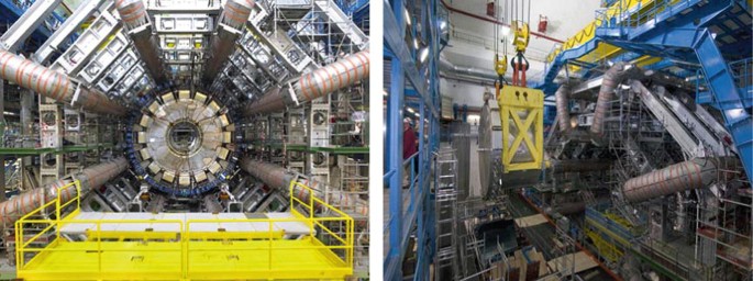

  

  Left: picture of the ATLAS barrel toroid superconducting magnet with its eight coils of 25 m length and of the ATLAS barrel calorimeter with its liquid Argon electromagnetic calorimeter and its scintillating tile hadronic calorimeter, as installed in the experimental cavern. Right: picture of the first end-cap LAr cryostat, including the electromagnetic, hadronic and forward calorimeters, as it is lowered into its docking position on one side of the ATLAS pit

  Fig. 16.4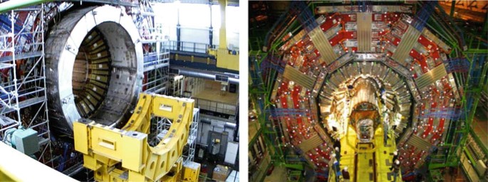

  

  Left: picture of the CMS superconducting solenoid, as integrated with the barrel muon system (outside) and with the barrel hadron calorimetry (inside). Right: picture of the insertion of the CMS silicon-strip tracker into the barrel crystal calorimeter

• the commissioning of the experiments with cosmic rays began in 2006, with the biggest campaigns in 2008 and 2009. These have yielded a wealth of initial results on the performance of the detectors in situ, a very important asset to ensure a rapid commissioning of the detectors for physics with collisions;

• the next commissioning step was achieved in an atmosphere of great excitement with first collisions at the injection energy of 900 GeV of the LHC machine and with very low luminosities of the order of 10²⁶−10²⁷ cm⁻²s⁻¹. All detector components were able to record significant samples of data, albeit at low energy and with insufficient statistics to fully commission the trigger and reconstruction algorithms dedicated to provide the signatures required for the initial Standard Model measurements and searches for new physics.

In parallel with the rapidly evolving integration, installation and commissioning effort at the experimental sites, the collaborations have also reorganised themselves to evolve as smoothly and efficiently as possible from a distributed construction project with a strong technical co-ordination team to a running experiment with the emphasis shifting to monitoring of the detector and trigger operation, understanding of the detector performance in the real LHC environment and producing the first physics results. A small but significant part of the human and financial resources are already focusing on the necessary upgrades to the experiments required by the LHC luminosity upgrade programme.

This chapter has been structured in the following way: Sect. 16.2 presents an overview of the ATLAS and CMS projects in terms of their main design characteristics, describes briefly the magnet systems, and summarises the main lessons learned from the 15-year long research and development and construction period. The next three sections, Sects. 16.3–16.5, describe in more detail the main features and challenges related respectively to the inner tracker, to the calorimetry and to the muon spectrometer, in the specific case of the ATLAS experiment. The subsequent two sections, Sects. 16.6 and 16.7, discuss in broad terms the various aspects of, respectively, the trigger and data acquisition system and the computing and software, again in the context of the ATLAS experiment. The next section, Sect. 16.8, summarises and compares briefly the expected performances at the time of beginning of data-taking of the main ATLAS and CMS systems. The last and final section, Sect. 16.9, gives a very brief overview of the performance and physics results achieved over the past 10 years.

16.2 Overall Detector Concept and Magnet Systems

This section presents an overview of the ATLAS and CMS detectors, based on the main physics arguments which guided the conceptual design, and describes the magnet systems, which have driven many of the detailed design aspects of the experiments.

16.2.1 Overall Detector Concept

Figures 16.5 and 16.6 show the overall layouts respectively of the ATLAS and CMS detectors and Table 16.2 lists the main parameters of each experiment. Both experiments are designed somewhat as cylindrical onions consisting of:

• an innermost layer devoted to the inner trackers, bathed in a solenoidal magnetic field and measuring the directions and momenta of all possible charged particles emerging from the interaction vertex;

  Fig. 16.5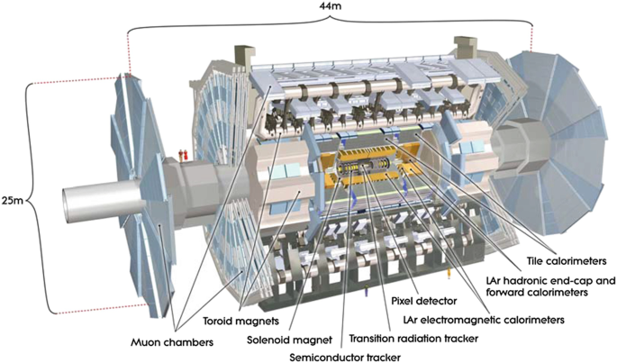

  

  Overall layout of the ATLAS detector

  Fig. 16.6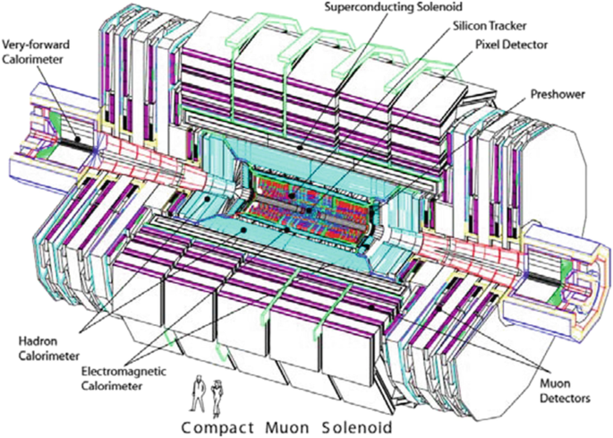

  

  Overall layout of the CMS detector

  Table 16.2 Main design parameters of the ATLAS and CMS detectors

• an intermediate layer consisting of electromagnetic and hadronic calorimeters absorbing and measuring the energies of electrons, photons and hadrons;

• an outer layer dedicated to the measurement of the directions and momenta of high-energy muons escaping from the calorimeters.

To complete the coverage of the central part of the experiments (often called barrel), so-called end-cap detectors (calorimetry and muon spectrometers) are added on each side of the barrel cylinders.

The sizes of ATLAS and CMS are determined mainly by the fact that they are designed to identify most of the very energetic particles emerging from the proton-proton collisions and to measure as efficiently and precisely as feasible their trajectories and momenta. The interesting particles are produced over a very wide range of energies (from a few hundred MeV to a few TeV) and over the full solid angle. They need therefore to be detected down to very small polar angles (θ) with respect to the incoming beams (a fraction of a degree, corresponding to pseudorapidities η of up to 5, where η = −log[tan(θ∕2)]; pseudorapidity is more commonly used at hadron colliders because the rates for most hard-scattering processes of interest are constant as a function of η). Most of the energy of the colliding protons is however dissipated in shielding and collimators close to the focussing quadrupoles (on each side of the experimental caverns, which house the experiments). The overall radiation levels will therefore be very high: many components in the detectors will become activated and will require special handling during maintenance, particularly near the beams.

For all the above reasons, both experiments have been designed following similar guiding principles:

• No particle of interest should escape unseen (except neutrinos, which will therefore be identified because their presence will cause an imbalance in the energy-momentum conservation laws governing the interactions measured in the experiments). The consequences of this simple statement are profound and far-reaching when one goes beyond simple sketches and simulations to the details of the real experiment:

  • successful operation of detectors able to measure the energies of particles with polar angles as small as one degree with respect to the incoming beams has required quite some inventiveness in material technology and a lot of detailed validation work to qualify the so-called forward calorimeters in terms of the very large radiation doses and particle densities encountered so close to the beams. Similar issues have been addressed of course very early on for the trackers, the main concerns being damage to semi-conductors (sensors and integrated circuits) and ageing of gaseous detectors. Even the muon detectors, to the initial surprise of the community, were confronted with irradiation and high-occupancy issues from neutron-induced cavern backgrounds pervading the whole experimental area;

  • avoiding any cracks in the acceptance of the experiment (especially cracks pointing back to the interaction region) has been a challenge of its own in terms of minimising the thickness of the LAr cryostats in ATLAS and of properly routing the large number of cables required to operate the ATLAS and CMS inner trackers;

  • if no particle can escape from the large volumes occupied by the experiments, then it becomes very hard for human beings to enter for rapid maintenance and repair. The access and maintenance scenarios for both experiments are quite complex and any major operation will only be feasible during long shutdowns of the accelerators. The detector design criteria have therefore become close to those required for space applications in terms of robustness and reliability of all the components.

• The high particle fluxes and harsh radiation conditions prevailing in the experimental areas have forced the collaborations to foresee redundancy and robustness for the measurements considered to be most critical. A few of the most prominent examples are described below:

  • CMS has chosen the highest possible magnetic field (4 T) combined with an inner tracker consisting solely of Silicon pixel detectors (nearest to the interaction vertex) and of Silicon microstrip detectors providing very high granularity at all radii. The occupancy of these detectors is below 2–3% even at the LHC design luminosity and the impact of pile-up is therefore minimal;

  • ATLAS has invested a very large fraction of its resources into three super-conducting toroid magnets and a set of very precise muon chambers, constantly monitored with optical alignment devices, to measure the muon momenta very accurately over the widest possible coverage (|η| < 2.7) and momentum range (4 GeV to several TeV). This system provides a stand-alone muon momentum measurement of sufficient quality for all benchmark physics processes up to the highest luminosities envisaged for the LHC operation;

  • Both experiments rely on a versatile and multi-level trigger system to make sure the events of interest can be selected in real time at the highest possible efficiency.

• Efficient identification with excellent purity of the fundamental objects arising from the hard-scattering processes of interest is as important as the accuracy with which their four-momenta can be determined. Electrons and muons (and to a lesser extent photons and τ-leptons with their decay products) provide excellent tools to identify rare physics processes above the huge backgrounds from hadronic jets. The requirements at the LHC are far more difficult to meet than at the Fermilab Tevatron: for example, at a transverse momentum of 40 GeV, the electron to jet production ratio decreases from almost 10⁻³ at the Tevatron to a few 10⁻⁵ at the LHC, because of the much larger increase of the production cross section for QCD hadronic jets than for W and Z bosons.

  For reasons of size, cost and radiation hardness, both experiments have limited the coverage of their lepton identification and measurements to the approximate pseudorapidity range |η| < 2.5 (or a polar angle of 9.4^∘ with respect to the beams). The implementation of these requirements has also had a very large impact on the design and technology choices of both experiments:

  • the length of the ATLAS and CMS super-conducting solenoids has been largely driven by the choices made for the lepton coverage;

  • ATLAS has chosen a variety of techniques to identify electrons, based first and foremost on the electromagnetic calorimeter with its fine segmentation along both the lateral and longitudinal directions of shower development, then on energy-momentum matching between the calorimeter energy measurement and the inner tracker momentum measurement, but enhanced significantly over most of the solid angle by the transition radiation tracker ability to separate electrons from charged pions. In contrast, CMS relies on the fine lateral granularity of its crystal calorimeter and on the energy-momentum matching with the inner tracker;

  • CMS has privileged the accuracy of the electron energy measurement with respect to the identification power with their choice of crystal calorimetry. The intrinsic resolution of the CMS electromagnetic (EM) calorimeter is superb with a stochastic term of 3–5.5% (see Sect. 16.8.2.1 for quantitative plots illustrating the performance) and the electron identification capabilities are sufficient to extract the most difficult benchmark processes from the background even at the LHC design luminosity.

• The overall trigger system of the experiments must provide a total event reduction of about 10⁷ at the LHC design luminosity, since the number of inelastic proton-proton collisions will occur at a rate of about 10⁹ Hz, whereas the storage capabilities will correspond to approximately 100 Hz for an average event size of 1–2 MBytes. Even today’s state-of-the art technology is however far from approaching the performance required for taking a trigger decision in the very small amount of time between successive bunch crossings (25 ns).

  The first level of trigger (or L1 trigger) in the ATLAS and CMS experiments is based on custom-built hardware extracting as quickly as possible the necessary information from the calorimeters and muon spectrometer and provides a decision in 2.5 to 3 μs, during which most of the time is spent in signal transmission from the detector (to make the trigger decision) and to the detector (to propagate this decision back to the front-end electronics). This reduces the event rate to about 100 kHz with a very high efficiency for most of the events of interest for physics analysis. During this very long (for relativistic particles) time, the hundreds of thousands of very sensitive and sophisticated radiation-hard electronics chips situated throughout the detectors have to store the successive waves of data produced every 25 ns in pipelines and keep track of the time stamps of all the data so that the correct information can be retrieved when the decision from the L1 trigger is received. The synchronisation of a vast number of front-end electronics channels over very large volumes has been a major challenge for the design of the overall trigger and timing control of the experiments.

16.2.2 Magnet Systems

The magnet systems of the ATLAS and CMS experiments [14] were at the heart of the conceptual design of the detector components and they have driven many of the fundamental geometrical parameters and of the broad technology choices for the components of the detectors. The large bending power required to measure muons of 1 TeV momentum with a precision of 10% has led both collaborations to choose superconducting technology for their magnets to limit the size of the experimental caverns and the overall costs. The choice of magnet system for CMS was based on the elegant idea of fulfilling at the same time with one magnet a high magnetic field in the tracker volume for all precision momentum measurements, including muons, and a high enough return flux in the iron outside the magnet to provide a muon trigger and a second muon momentum measurement for the experiment. This is achieved with a single solenoid of a large enough radius to contain most of the CMS calorimeter system. In contrast, the choice of magnet system for ATLAS was driven by the requirement to achieve a high-precision stand-alone momentum measurement of muons over as large an acceptance in momentum and η-coverage as possible. This is achieved using an arrangement of a small-radius thin-walled solenoid, integrated into the cryostat of the barrel electromagnetic calorimeter, surrounded by a system of three large air-core toroids, situated outside the ATLAS calorimeter systems and generating the magnetic field for the muon spectrometer. The main parameters of these magnet systems are listed in Table 16.3 and their stored energies are compared to those of previous large-scale magnets in high-energy physics experiments in Fig. 16.7.

Fig. 16.7

Ratio of stored energy over mass, E∕M, versus stored energy, E, for various magnets built for large high-energy physics experiments

Table 16.3 Main parameters of the CMS and ATLAS magnet systems

In CMS, the length of the solenoid was driven by the need to achieve excellent momentum resolution over the required η-coverage and its diameter was chosen such that most of the calorimetry is contained inside the coil. In ATLAS, the position of the solenoid in front of the barrel electromagnetic calorimeter has demanded a careful optimisation of the material in order to minimise its impact on the calorimeter performance and its length has been defined by the design of the overall calorimeter and inner tracker systems, leading to significant non-uniformity of the field at the end of the tracker volume.

The main advantages and drawbacks of the chosen magnet systems can be summarised as follows, considering successively the inner tracker, calorimeter and muon system performances (see Sect. 16.8):

• the higher field strength and uniformity of the CMS solenoid provide better momentum resolution and better uniformity over the full η-coverage for the inner tracker;

• the position of the ATLAS solenoid just in front of the barrel electromagnetic calorimeter limits to some extent the energy resolution in the region 1.2 < |η| < 1.5;

• the position of the CMS solenoid outside the calorimeter limits the number of interaction lengths available to absorb hadronic showers in the region |η| < 1;

• the muon spectrometer system in ATLAS provides an independent and high-accuracy measurement of muons over the full η-coverage required by the physics. This requires however an alignment system with specifications an order of magnitude more stringent (few tens of μm) than those of the CMS muon spectrometer. In addition, the magnetic field in the ATLAS muon spectrometer must be known to an accuracy of a few tens of Gauss over a volume of close to 20,000 m³. The software implications of these requirements are non-trivial (size of map in memory, access time);

• the muon spectrometer system in CMS has limited stand-alone measurement capabilities and this affects the triggering capabilities for the luminosities envisaged for the LHC upgrade.

In terms of construction, the magnet systems have each turned out to be a major project in its own right with very direct and strong involvement from the Technical Coordination team [15] and from major national laboratories and funding agencies. A detailed account of the construction of these magnets is beyond the scope of this review and this section can be concluded by simply stating that during the course of the past few years, all these magnets have undergone very successfully extensive commissioning steps, sustained operation at full current, in particular for cosmic-ray data-taking in 2008/2009, and stable operation with beam in the LHC machine at the end of 2009.

16.2.2.1 Radiation Levels

At the LHC, the primary source of radiation at full luminosity comes from collisions at the interaction point. In the tracker, charged hadron secondaries from inelastic proton-proton interactions dominate the radiation backgrounds at small radii while further out other sources, such as neutrons, become more important. Table 16.4 shows projected radiation levels in key areas of the detector.

Table 16.4 The 1 MeV neutron equivalent fluence (F _neq) and doses in key areas of the ATLAS detector after 500 fb⁻¹ of data (estimated to be approximately 7 years of operation at design luminosity)

In ATLAS, most of the energy from primaries is dumped into two regions: the TAS (Target Absorber Secondaries) collimators protecting LHC quadrupoles and the forward calorimeters. The beam vacuum system spans the length of the detector and in the forward region is a major source of radiation backgrounds. Primary particles from the interaction point strike the beam-pipe at very shallow angles, such that the projected material depth is large. Studies have shown that the beam-line material contributes more than half of the radiation backgrounds in the muon system. The deleterious effects of background radiation fall into a number of general categories: increased background and occupancies, radiation damage and ageing of detector components and electronics, single-event upsets and single-event damage, and creation of radionuclides which will impact access and maintenance scenarios.

16.2.3 Lessons Learned from the Construction Experience

It is fair to say that most of the physicists and engineers involved in the ATLAS and CMS construction were faced with a challenge of this scope and size for the first time. It seems therefore appropriate to put some emphasis in this article on the lessons learned from the construction of these detectors. This section describes the general lessons learned and the next sections will give more explicit examples in many cases when describing the experience from the construction of the detector components.

The lessons learned are of varying nature, many are organisational, many are technical and some are sociological. Some are specific to the LHC, some are specific to the way international high-energy physics collaborations work, and some are of a general enough nature that they might well apply to any complex high-tech project of this size. It is therefore hard to classify them in a clear logical order, and this review has attempted to rank them from the general and common to the specific and unique to the LHC.

16.2.3.1 Time-Scales, Project Phases and Schedule Delays

If there has been one lesson learned from the days in the early 1990s when ATLAS and CMS came into being as detector concepts, it is certainly that the research and development phase of projects of this complexity are impossible to plan with real certainty about the time-scales involved. Modern tools for project management are of little help here because the vagaries of the initial phase do not generally obey the simple laws of project schedules and charts. These can be a posteriori explained of course:

• the research and development phase for new high-tech detector elements, such as radiation-hard silicon sensors and micro-electronics, crystals grown from a new material, large-scale electrodes for operation at high voltage in liquid Argon, etc., will always be a phase to which one has to allocate as much time as feasible within the overall project schedule constraints. The justification for this is basically that the potential rewards are enormous, as was exemplified by the late but striking success of the deep sub-micron micro-electronics chips pioneered by CMS and now used throughout all LHC experiments, and by the late but successful operation of CMS PbWO₄ crystals with their avalanche photodiode readout and associated electronics. Making the appropriate research and development choices at the right time will however always remain a challenge for any new project of this scope and complexity.

• less known to many colleagues in our community is the phase during which the components for producing complex detector modules are launched for manufacturing in industry. This phase can indeed be planned correctly if the required physicist/engineering experience is available, if the funding allows for multiple suppliers to mitigate potential risks, and if the physicists agree quickly to moderate their usually very demanding specifications to adapt them to the actual capabilities of industry.

  Experience has shown however that success was far from guaranteed in this phase, with causes for delays or outright initial failures ranging from being forced to award contracts to the lowest bidder, to incomplete technical specifications, to handling and packaging issues during manufacturing, particularly for polyimide-based products, of which there are many thousands of m² in both experiments. This material shows up under various forms (especially in flexible printed circuit boards for various applications) and is a basic insulating material with excellent electrical and mechanical properties, with very high tolerance to radiation, but unfortunately also with a high propensity to absorb moisture and thereby lead to unexpected changes in even the course of a well-defined manufacturing process. Serious technical problems in this area have affected the manufacturing schedule of major components of both experiments (hybrids for semi-conductor detectors, flexible parts of printed-circuit boards, large-size electrodes for electromagnetic calorimetry), but other issues such as welding, brazing and general integrity and leak-tightness of thin-walled cooling pipes have also been a concern for several of the components in each experiment.

  In addition, several of the more significant contracts were seriously affected by changes in the industrial boundary conditions (insolvency, change of ownership). The recommended purchasing strategy of having multiple suppliers for large contracts, to minimise the consequences from a possible failure in the case of a single supplier, has not always been the optimal one (high-quality silicon sensors are perhaps the most prominent example).

The detailed construction planning can be consulted in the various Technical Design Reports (TDR), most of which were submitted from 1996 to 1998 to seek approval for construction of the major detector components. This called for completion of this construction phase by mid-2001 to mid-2003. At the time when a big schedule and financial crisis shook the LHC project in fall 2001 (see below), it was already clear that many detector components would not be on schedule by a significant margin.

The 2-year delay in the completion of the accelerator resulting from this crisis was also needed by the experiments, as can be seen from Table 16.5, which illustrates the major construction milestones originally planned at the time of the TDRs and actually achieved. When trying to assess the significance of the differences between the dates achieved for the delivery of major components of the experiments and those planned 9 years ago, it is important to remember the prominent events, at CERN and within the collaborations, which happened during these years:

• at the time of the submission of the various TDRs for ATLAS and CMS, the construction and installation schedule was worked out top-down, based on a ready-for-operation date of summer 2005 for the LHC machine and the experiments;

  Table 16.5 Main construction milestones for the ATLAS and CMS detectors

• in 1999, the CMS collaboration decided to replace the micro-strip gas chamber baseline technology for the outer part of their Inner Detector by “low-cost” silicon micro-strip detectors. This is probably the most outstanding example of decisions, which the collaborations had to take after the TDRs were submitted and which have affected the construction schedule in a major way;

• in 2001, when the CERN laboratory management announced significant cost overruns, mostly in the machine, but also in the ATLAS and CMS experiments, it also announced a 2-year delay in the schedule for the machine, which obviously led to a readjustment of the construction and installation schedule of the experiments. By that time, both in ATLAS and CMS, the Technical Co-ordination teams had worked out a realistic installation schedule, which still needed to be fleshed out substantially in areas such as services installation, commissioning of ancillary equipment for operation of the huge devices to be operated underground, etc.;

• the ATLAS experimental cavern was delivered more or less on time in spring 2003, whereas the CMS experimental cavern suffered considerable delays and was delivered only towards the end of 2004.

16.2.3.2 Physicists and Engineers: How to Strike the Right Balance?

This is a very delicate issue because there exists no precise recipe to solve this problem. The ATLAS and CMS experiments were born from the dreams of physicists but are based today on the calculations and design efforts from some of the best teams of engineers and designers in the world. One should not forget that, originally (in 1987), even the physicists thought that only a muon spectrometer behind an iron dump was guaranteed to survive the irradiation and that most tracking technologies were doomed at the highest luminosities of the LHC [16].

Although a strong central and across-board (from mechanics to electronics, controls and computing) engineering effort would have been desirable from the very start (i.e. around 1993), a standard centralised and very systematic engineering approach alone, as is frequently used in large-scale astronomy projects, could not have been used for several reasons:

• the cost would have been prohibitive;

• only the physicists can actually make the sometimes difficult choices and decisions when faced with problems requiring certain heart-wrenching changes in the fundamental parameters of the experiment (number of layers in the tracking detectors, number of cells in the electromagnetic calorimeter, overall strength and uniformity of the magnetic field, etc.). The number of coils to be constructed in the ATLAS superconducting toroid and the peak field of the CMS central solenoid are two examples of early and fundamental parameters of the experiments, which were studied for quite some time and had a significant bearing on the overall cost of the experiments;

• some of the usual benefits of such an approach, such as optimised production costs for repetitive manufacturing of the same product, are not there to be reaped when considering the experiments as a whole rather than looking at individual components, such as the micro-strip silicon modules, which number in many thousands and did indeed benefit in many aspects from a systematic engineering approach;

• the overall technological scope of these nascent experiments required creativity and novel approaches in areas as far apart as 3D-calculations of magnetic fields and forces over very large volumes containing sometimes unspecified amounts of magnetic materials and radiation-dose and neutron-fluence calculations of unprecedented complexity in our field to evaluate the survival of a variety of objects, from the basic materials themselves to complex micro-electronics circuits. Only a well-balanced mix of talented and dedicated designers, engineers and physicists could have tackled such issues with any chance of success;

• the decision-making processes in our community cannot be too abrupt. Consensus needs to be built, especially between physicists but also between engineers from sometimes widely different cultures and backgrounds.

In retrospect, however, there has emerged as a clear lesson, that the management of the experiments should have evolved at an earlier stage the decision-making process from a physicist-centric one at the beginning, when little was known about the detailed design of all the components, to a more engineer-centric one, as the details were fleshed out more and more. Establishing engineering envelopes and assembly drawings for the different systems, routing the very large and diverse amount of services needed to operate complex detectors distributed everywhere across the available space, and designing, validating and procuring common solutions for many of the electronics and controls components are examples, which clearly illustrate this need. The collaborations have indeed encountered difficulties to recognise such needs and to react to them at the appropriate moment in time.

16.2.3.3 International and Distributed: A Strength or a Weakness?

ATLAS and CMS are truly international and distributed collaborations, even if the engineering and/or manufacturing of some of the major components of both experiments have been entrusted to large laboratories situated all across the world. Modern technology (web access to document servers, video-conferencing facilities, more uniform standards, such as the use of the metric system, for drawings, specifications and quality assurance methods, electronic reporting tools) has been instrumental in improving the efficiency of the various strands of these collaborations, an admittedly weak point of such organisations. There are two major weaknesses intrinsic to collaborations structured as ATLAS and CMS with distributed funding resources:

• one is that it is not simple to converge on the minimum required number of technologies once the research and development phase is over. One example of perhaps unnecessary multiplication of technologies are the precision chambers in the ATLAS muon spectrometer, where the highest-η part of the measurements are covered by cathode strip chambers rather than the monitored drift tube technology used everywhere else. A similar example can be found in the CMS muon spectrometer, which is also equipped with two different chamber technologies in the barrel and end-cap regions (see Sect. 16.5).

• the decision-making process is sometimes skewed by the difficulty of conveying a global vision of the best interests of the project, which should be weighed against the more localised and focussed interests of particular funding agencies, some of which operate within a rather inflexible legal framework.

The strengths of this international and distributed approach far outweigh however its deficiencies over a much more centralised one, such as that adopted for the Super-Conducting Super Collider with a centralised funding and management in Waxahachie (Texas) about 15 years ago:

• the flexibility achieved has often provided solutions to the inevitable problems, which have shown up during the design and construction phase. Whenever a link in the chain was shown to falter or even to be totally missing, the collaboration has often been able to find alternate solutions. If a large laboratory had difficulties in meeting a complex technological challenge alone because of limitations in funding and human resources, other laboratories with similar expertise could be sought out and integrated into the effort with minimal disruption. If the production line for certain detectors did not churn out the required number of modules per unit time because of yield issues or of an underestimate of the human resources required, other production lines, often on different continents with cheaper labour costs, were launched and operated successfully.

• many concrete examples have shown that motivation and dedication to the project go together with the corresponding responsibilities, both technical and managerial. It is worthwhile also to note here that it surely would have been beneficial for the overall LHC project if the management of the ATLAS and CMS experiments would have been integrated as a real partner into the CERN management structure at the highest level right from the beginning. Both experiments were severely handicapped by a cost ceiling without contingency defined top-down more than 10 years ago.

  It is fair to say that, without the motivation and dedication of many of our colleagues all over the world, who fought and won their own battles at all required levels (technical, funding, human resources, organisational), and of their funding agencies, the construction of ATLAS and CMS would not have reached its astounding and successful completion with only small parts of each experiment deferred. Dealing with significant deferrals has always been damaging to the atmosphere of large collaborations of this type and the fact that both experiments are now essentially complete should certainly be attributed to the credit of all their participants.

  A particular mention should go here to our Russian colleagues, who have not only strongly contributed intellectually to the experiments, as all the others, from the very beginning, but who also staffed continuously, together with other Eastern European colleagues and also colleagues from Asia, a very large fraction of the teams needed to assemble, equip, test and commission the major detector components. This was quite striking during the installation period from just listening to the conversations occurring in the lifts bringing people and equipment up and down the experimental shafts.

• the concept of deliverables has also turned out to the advantage of the projects. Each set of institutes in each country have been asked to deliver a certain fraction of specific components of the detector systems, ranging from a modest (but critical!) scope, such as the fabrication of the C-fibre cylinders for the barrel semi-conductor tracker in ATLAS, to a very large (and very visible to the whole collaboration!) scope, such as the CMS crystal production in several commercial companies, or as the ATLAS super-conducting solenoid built in Japanese industry, in close collaboration with institutes from the same country, which are full-fledged members of the collaboration.

  This concept has certainly maximised the overall funding received by ATLAS and CMS, because each funding agency has to a certain extent been asked and has agreed to take responsibility for the delivery of certain detector components without assigning to these a specific cost, since the real costs vary from country to country, and even the ratios of costs between different countries inevitably vary, because of the approximately uniform costs of raw materials as compared to the wildly differing costs of skilled and unskilled labour. Since the infrastructure of the experiments is a mixture of low and high technology components, most participating countries have in the end been able to contribute efficiently in kind to the common projects of interest to the whole collaboration.

• the scheme based on deliverables rather than raw funding could not have worked however without being completed by a sizable set of common projects, to which the funding agencies had to contribute, either through funds to be handled by the management of the experiments, either through in-kind contributions, the cost of which was determined in the context of the same scheme as for the deliverables. Examples of these common projects are the magnets of both experiments, the LAr cryostats and cryogenics of ATLAS, and much of the less high-tech infrastructure components of both experiments.

• finally, the computing operations of the experiments and the analysis of the data taken over the next 10 years do and will require a very distributed and international style of working also. This is not really new to our community, it is just of an unprecedented scale in size and duration. The collaborations are evolving now from an organisational model focussed initially on research and development and then on construction to a new model, which is focussed more on detector operation, monitoring of the data quality and data preparation, leading to the analysis work required to understand precisely the behaviour of the detectors and extract as efficiently as possible the exciting physics ahead of us. The years spent together and the difficulties overcome over a 15-year long period of design and construction have certainly cemented the collaborations in a spirit of respect and mutual understanding of all their diverse components. This will surely turn out to be an excellent preparation for the forthcoming challenges when faced with real experimental data.

16.2.3.4 A Well Integrated and Strong Technical Co-ordination Team

It is clear that without such a team the experiments would most probably have faced insurmountable construction delays and integration problems. The Technical Co-ordination team must in a sense be perceived as the strong backbone of the experiment by all the physicists in the community. This was indeed the case in the installation phase of the experiments, at a time when it had to smoothly execute a complex suite of integration and installation operations for detector components arriving from all over the world. But this was less the case 10–15 years ago, at a time when the physicists and engineers in this team were sometimes perceived as a nuisance disrupting the delicate balance of the collaboration and were criticised in different ways:

• many physicists and engineers had great trouble when asked to specify all the details of cables, pipes and connectors, at a very early time (15 years ago) when they were desperately trying to move into mass production;

• strong resistance to reviews was encountered, based on partially correct, but also partially fallacious, arguments that all the expertise in a given area was already available in the project under review;

• the multiplicity of reviews also caused sometimes considerable friction and frustration, especially since an overall co-ordination between funding agency reviews and internal project reviews was almost impossible to put into place.

In retrospect, these reviews are indeed necessary, whether or not all of their recommendations and outcomes have turned out to be of a specific concrete usefulness, because they have usually forced the project teams to collect documentation, take stock, step back and think about issues sometimes obscured by the more immediate and pressing problems at hand.

Although the construction of the individual detector components can be argued to have been quite successful under the umbrella of deliverables and in the absence of a fully centralised management of the experiment resources, there are obviously a variety of tasks, which have to be solved by a strong centralised team of designers, engineers and physicists. As in any such process, this team is much better accepted if it is built up at least partially from people within the collaboration, who are already well integrated in and known to the collaboration. Despite all the grumbling and moaning, the efforts of the Technical Co-ordination team have been crucial to the success of the ATLAS and CMS projects:

• finding common (often commercial) solutions does not come easily to large numbers of inventive and often opinionated physicists. Common solutions across the experiments are even harder to achieve, although they have turned out to be profitable to all parties in a number of areas. Clearly the strong research and development programme launched in 1989 by CERN for the development of the LHC detector technologies has been a key element in the definition of the various detector concepts (radiation-hard silicon detectors and electronics, electromagnetic and hadronic calorimetry, various tracking technologies, etc.).

  In the areas where such common (often commercial) solutions have been adopted in many cases in the past, the successes of the research and development programme have been less spectacular (data transmission, specialised trigger processors, various offline software developments), most probably because the solutions emerging today were not easy to predict from the technology trends of 20 years ago, when the worldwide web, mobile phones, inexpensive desktop computing and high-speed networks did not exist.

  The Technical Co-ordination team has certainly been very instrumental in encouraging the collaboration to adopt common technical solutions and has also delegated to the appropriate persons in the collaboration the mandate to negotiate and agree these common solutions across the experiments: the frame contracts with major micro-electronics suppliers, the gas systems, the power supplies, the electronics crates and racks and the slow controls infrastructure hardware and database software can be quoted as some of the more prominent examples.

• establishing a strong quality assurance and review process across the whole collaboration is a must at an early stage in such complex projects, where standard commercial products have often failed, sometimes for multiple reasons owing to the boundary conditions in the experimental caverns (radiation background and magnetic field).

  As stated above, the review process (from conceptual engineering design reviews, to production readiness and production advancement reviews) can be very beneficial and even well accepted within the collaboration if it is kept lightweight and perceived as executed by people involved in the project as all the others rather than by an elite breed of top-level managers.

  Most of the ATLAS and CMS Technical Design Reports quoted as references in this review address quality assurance with ambitions and specifications, which are fully justified on paper but much harder to implement in reality when facing time pressure and the inevitable lack of human resources to fulfill every aspect of the task. In relation to industry in particular, the effort required in monitoring production of delicate components had been totally underestimated or even ignored in the design phase. The reviews put in place by the Technical Co-ordination team have played an important role in keeping all aspects related to schedule, resources and quality assurance under control during the detector construction. They have also ensured that large groups with significant project responsibilities were not allowed to operate for too long in a stand-alone mode without synchronising with and reporting back to Technical Co-ordination, the management of the experiments and the collaboration at large. The risks involved in letting things go astray too much are simply unacceptable for projects of this complexity and size.

• As stated above, one weakness perhaps of the multiple dimensions under which ATLAS and CMS are viewed is that the funding agencies have often conducted their own necessary review processes in a way largely decoupled from the review process operated by the management of the experiments. This weakness stems from the lack of central control of expenditures because of the distributed funding and spending responsibilities. This can obviously lead to inefficiencies in the actual execution of the project and, worse, sometimes to conflicting messages given to the institutes concerning priorities, since those of a given funding agency may not always coincide with those of the experiment. The common funds necessary to the construction of significant components of the experiments, such as magnets, infrastructure, shielding, cryostats, etc., are a prominent example which comes to mind, when assessing which of the components of the experiments had the most difficulty in dealing with the multi-threaded environment, in which the detector construction has been achieved.

Finally, it is in the very recent phase of assembly, installation and commissioning of the ATLAS and CMS detectors that the enormous efforts and contribution from the Technical Co-ordination teams have been most visible: they have had to organise the vast teams of sub-contractors and specialised personnel from the collaborating institutes and they have had to deal with the daily burden of making sure all the tasks were executed as smoothly as possible with safety as one of the paramount requirements.

16.3 Inner Tracking System

16.3.1 Introduction

The ATLAS tracker is designed to provide hermetic and robust pattern recognition, excellent momentum resolution and both primary and secondary vertex measurements [17] for charged tracks above a given p _T threshold (nominally 0.5 GeV, but as low as 0.1 GeV in some ongoing studies of initial measurements with minimum-bias events) and within the pseudorapidity range |η| < 2.5. It also provides electron identification over |η| < 2.0 and a wide range of energies (between 0.5 and 150 GeV). It is contained within a cylindrical envelope of length ±3512 mm and of radius 1150 mm, within the solenoidal magnetic field of 2 T. Figures 16.8 and 16.9 show the sensors and structural elements traversed by 10 GeV tracks in respectively the barrel and end-cap regions.

Fig. 16.8

Drawing showing the sensors and structural elements traversed by a charged track of 10 GeV p _T in the ATLAS barrel inner detector (η = 0.3). The track traverses successively the beryllium beam-pipe, the three cylindrical silicon-pixel layers with individual sensor elements of 50 × 400 μm², the four cylindrical double layers (one axial and one with a stereo angle of 40 mrad) of barrel silicon-microstrip sensors (SCT) of pitch 80 μm, and approximately 36 axial straws of 4 mm diameter contained in the barrel transition-radiation tracker modules within their support structure

Fig. 16.9

Drawing showing the sensors and structural elements traversed by two charged tracks of 10 GeV p _T in the ATLAS end-cap inner detector (η = 1.4 and 2.2). The end-cap track at η = 1.4 traverses successively the beryllium beam-pipe, the three cylindrical silicon-pixel layers with individual sensor elements of 50 × 400 μm², four of the disks with double layers (one radial and one with a stereo angle of 40 mrad) of end-cap silicon-microstrip sensors (SCT) of pitch ∼80 μm, and approximately 40 straws of 4 mm diameter contained in the end-cap transition radiation tracker wheels. In contrast, the end-cap track at η = 2.2 traverses successively the beryllium beam-pipe, only the first of the cylindrical silicon-pixel layers, two end-cap pixel disks and the last four disks of the end-cap SCT. The coverage of the end-cap TRT does not extend beyond |η| = 2

The ATLAS tracker consists of three independent but complementary sub-detectors. At inner radii, high-resolution pattern recognition capabilities are available using discrete space-points from silicon pixel layers and stereo pairs of silicon micro-strip (SCT) layers. At larger radii, the transition radiation tracker (TRT) comprises many layers of gaseous straw tube elements interleaved with transition radiation material. With an average of 36 hits per track, it provides continuous tracking to enhance the pattern recognition and improve the momentum resolution over |η| < 2.0 and electron identification complementary to that of the calorimeter over a wide range of energies.

Table 16.6 lists the main parameters of the ATLAS tracker:

• the radial position of the innermost measurement is essentially determined by the outer diameter of the beam pipe, which has been manufactured using expensive and delicate Beryllium material over an overall length of 7 m. The active part of the tracker has a half-length of 280 cm, slightly longer than that of its solenoid, resulting in significant field non-uniformities and momentum resolution degradation at each end.

  Table 16.6 Main parameters of the ATLAS tracker system

• the total power required for the tracker front-end electronics will increase from approximately 62 to 85 kW from initial operation to high-luminosity operation after irradiation. Bringing this amount of power to the detector requires large amounts of copper; the resulting heat load is very uniformly distributed across the entire active volume of the tracker and has to be removed using innovative techniques (fluor-inert liquids to mitigate the risks from possible leaks, thin-walled pipes made from light metals, evaporative techniques for optimal heat removal in the case of the silicon-strip and pixel detectors). There is also considerable heat created by the detectors themselves: the silicon-strip modules will dissipate about 1 W each from sensor leakage currents at the end of their lifetime, and the highest-occupancy TRT straws dissipate about 10 mW each at the LHC design luminosity.

• for all of the above reasons, it has been well known since the early 90’s in the LHC community that the material budget of the tracker systems as built would pose serious problems in terms of their own performance (see Sect. 16.8.1) and even more so in terms of the intrinsic performance of the electromagnetic calorimeter and of the overall performance for electron/photon measurements (see Sect. 16.8.2). Despite the best efforts of the community, the material budget for the tracker has risen steadily over the years and reached values of two radiation lengths (X₀) and close to 0.6 interaction lengths (λ) in the worst regions (see Sect. 16.3.2.1 for more details and plots).

The high-radiation environment imposes stringent conditions on the inner-detector sensors, on-detector electronics, mechanical structure and services. Over the 10-year design lifetime of the experiment, the pixel inner vertexing layer must be replaced after approximately 3 years of operation at design luminosity. The other pixel layers and the pixel disks must withstand a 1 MeV neutron equivalent fluence F_neq [18] of up to ∼8 × 10¹⁴ cm⁻². The innermost parts of the SCT must withstand F_neq of up to 2 × 10¹⁴ cm⁻². To maintain an adequate noise performance after radiation damage, the silicon sensors must be kept at low temperature (approximately − 5 to − 10^∘C) implying coolant temperatures of ∼−25^∘C. In contrast, the TRT is designed to operate at room temperature.

The above operating specifications imply requirements on the alignment precision which are summarised in Table 16.7 and which serve as stringent upper limits on the silicon-module build precision, the TRT straw-tube position, and the measured module placement accuracy and stability.

Table 16.7 Intrinsic measurement accuracies and mechanical alignment tolerances for the tracker sub-systems, as defined by the performance requirements of the ATLAS experiment

This leads to:

• (a) a good construction accuracy with radiation-tolerant materials having adequate detector stability and well understood position reproducibility following repeated cycling between temperatures of − 20 and + 20^∘C, and a temperature uniformity on the structure and module mechanics which minimises thermal distortions;

• (b) an ability to monitor the position of the detector elements using charged tracks and, for the SCT, laser interferometric monitoring [19];

• (c) a trade-off between the low material budget needed for optimal performance and the significant material budget resulting from a stable mechanical structure with the services of a highly granular detector.

The design and construction of systems, capable of meeting the physics requirements and of providing stable and robust operation over many years, has been perhaps the most formidable challenge faced by the experiment because of the very harsh radiation conditions to be faced near the interaction point and of the conflicting requirements in terms of material budget between the physics and the design constraints. The latter arise mostly from the on-detector high-speed front-end electronics, which require a lot of power to be fed into a limited volume and therefore a large amount of heat to be removed from a very distributed set of local heat sources across the whole tracker.

This section describes briefly the ATLAS tracker and its main properties and discusses a few salient aspects from the construction experience and from the measured performance in laboratory and test beam of production modules in the various technologies. A few examples of the overall performance expected in the actual configuration of the experiment are presented in Sect. 16.8.1, where it is also compared to the expected performance of the CMS tracker.

16.3.2 Construction Experience

16.3.2.1 General Aspects

The ATLAS tracker system has evolved considerably since the submission of the Technical Proposal in 1994 and even since the corresponding Technical Design Reports in 1997/1998. The evolution was dictated by many factors, some of which have already been alluded to in Sect. 16.2.3 and some of which are related to the specific design challenges posed:

• the rapid development of radiation-hard silicon sensors and of their front-end electronics led many physicists and engineers in the community to focus for a long time on the single module scale and, as a consequence, to perhaps address some of the systems issues, especially for the readout and cooling aspects, too late.

• the legitimate concerns throughout the collaborations about the material budget of the tracker systems resulted in huge pressures on the engineering design effort in terms of materials at a very early stage. This effort has been largely successful in terms of mechanics, as can be seen from the very light and state-of-the-art structures used to support and hold the detector components in the tracker system. The already considerable experience from the space industry across the world turned out to be invaluable, including in terms of thermal behaviour and of resistance to radiation and to moisture absorption.

• the tracker macro-assemblies, once completed as operational devices, are the sum of a large number of diverse and tiny components. Many of these components were not built into the design from the very beginning and only general assumptions based on past experience were made concerning their manufacture. Several of these assumptions turned out to be incorrect: for example, the use of silver in the electrical connections and cables has had to be minimised because of activation issues. The pressure on the material budget led to the choice of risky technical solutions for cooling and power, involving hard-to-validate thin-walled Aluminium, copper/Nickel or Titanium pipes and polyimide/Aluminium tapes rather than the less risky but heavier stainless steel pipes and polyimide/copper tapes.

• many of the systems aspects were discovered as the detailed design progressed, rather than foreseen early on, and this has led to difficult retrofitting exercises and sometimes to technical solutions more complex and risky than those which would be devised from a clean slate today. Some of the substrates for the electronics of the silicon modules barely existed in terms of conceptual design at a time when the front-end electronics chip was ready for production. This is one example of a specific and critical component, which was not always incorporated into the detailed design of the system from the very beginning.

  Another more general example stems from the engineering choices made for the implementation of the on-detector and off-detector cooling systems: there are as many on-detector cooling schemes and pipe material choices as there are detector components. The cooling systems themselves are all operating under severe space limitations on-detector and at high pressure (from 3 to 6 bars). These systems range from room-temperature monophase C₆F₁₄ for the TRT to cold evaporative C₃F₈ for the SCT and pixels. Many problems have been encountered during the commissioning in situ and early operation of these systems, and it is fair to say a posteriori that this is one area where a stronger and more centralised engineering effort would have probably come up with a more uniform, more robust and redundant, and less risky implementation.

• Table 16.8 shows how optimistic the estimate of the material budget of the ATLAS tracker was at the time of the Technical Proposal in 1994 and how it has evolved since then to reach the values quoted in early 2008, after completion of the installation of all of its components. These values cannot be claimed to be final yet, although most of the remaining uncertainties are small and related to the exact routing details of the various services and of patch-panels for cable and pipe connections. These are situated within the tracker volume, but not always in the fiducial region where the detectors expect to perform precision tracking and electromagnetic calorimetry measurements (for example, the patch-panels for the pixel detector are outside this fiducial region). The material budget for the tracker has risen steadily over the years and the only significant decrease seen (from 1997 to now) is due to the rerouting of the pixel services from a large radius along the LAr barrel cryostat to a much smaller radius along the pixel support tube, a significant change in the ATLAS tracker design, which occurred in 1999.

  Table 16.8 Evolution of the amount of material expected in the ATLAS tracker from 1994 to 2007

  Figure 16.10 shows how this material budget is distributed as a function of pseudorapidity. The material closest to the beam (pixel detectors) is clearly the one most critical for the performance of the tracker and of the electromagnetic calorimetry: this amounts to between 10 and 50% X/X₀. The material budget can also be broken down in terms of its functional components: a large contribution to the material budget arises from cooling and cables in areas where these services accumulate to be routed radially outwards, towards the cracks in the electromagnetic calorimetry foreseen for their passage. It is therefore not surprising that, until all the details of the granularity, technical components, routing, fixation schemes, etc., were known and incorporated into assembly drawings and detailed spreadsheets, the material budgets announced for this tracker of unprecedented scope and complexity were largely underestimated.

  Fig. 16.10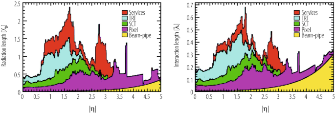

  

  Material distribution (X ₀, λ) at the exit of the ATLAS tracker, including the services and thermal enclosures. The distribution is shown as a function of |η| and averaged over ϕ. The breakdown indicates the contributions of external services and of individual sub-detectors, including services in their active volume. These plots do not include additional material just in front of the electromagnetic calorimeter, which is quite large in ATLAS (LAr cryostats and, for the barrel, solenoid coil)

16.3.2.2 Silicon-Strip and Straw Tube Trackers

The ATLAS SCT contains a total of 4088 modules corresponding to 6.3 million channels, of which 99.7% have been measured to be fully operational in terms of electrical and thermal performance in situ. The ATLAS TRT comprises approximately 350,000 channels, of which about 98.5% fully meet the operational specifications in terms of noise counting rate and of basic efficiency and high-voltage behaviour.

The ATLAS tracker was installed in three successive stages, from summer 2006 (barrel SCT/TRT tracker), to end 2006 (end-cap SCT/TRT trackers), and to spring 2007 (pixels). It is impossible to properly give credit here to all the work performed over the past 15 years to validate the design choices involving each and every one of the delicate components composing these tracking detectors. Only a few of the most prominent examples are quoted below:

• all the front-end electronic designs had to be submitted to stringent specifications in terms of survival to very high ionisation doses and neutron fluences and of robustness against single-event upsets. The performance of fully irradiated and operational modules equipped with the latest iteration in the design had to be repeatedly measured and characterised in laboratory tests and particle beams of various types and intensities [20].

• each component in contact with the active gas of the ATLAS TRT straws has had to be validated in a well-controlled set-up over many hundreds of hours of accelerated ageing tests using the gas mixture chosen for operation in the experiment. This was necessary because impurities of only a few parts per billion, picked up somewhere in the system, could be deposited on the wires and thereby destroy the gas gain in an irrecoverable way [21]. One critical component in the barrel TRT modules, a glass bead serving as wire joint to separate the two halves of each wire, actually failed the ageing tests with the originally chosen gas mixture (Xe–CO₂–CF₄) and the collaboration had to eventually change the gas mixture to the current one (Xe–CO₂–O₂), in which the fluorine component has been removed. This gas mixture reduces the direct risk to the wire joints, but is somewhat less stable operationally and does not have the same self-cleaning properties as the original one.

16.3.2.3 Pixel Detectors

The ATLAS pixel detector has been one of the last elements installed in the experiment, in great part for practical reasons, but also because this is the detector which has undergone the most difficult development path. It can perhaps be considered as the most striking example of the marvels achieved during the long and painstaking years of research and development: the pixel detector will survive over many years in the most hostile region of the experiment and deliver some of the most important data required to understand in detail what will be happening within a few tens of microns from the interaction point.

Fifteen years ago, at the time of the ATLAS Technical Proposal, very few physicists believed that these detectors could be built within the specifications required in terms of radiation hardness and of readout bandwidth and speed. Today, the data collected using cosmic rays (in 2008 and 2009) and early collisions (end of 2009) have demonstrated that the pixel detector works as expected. The future will tell how long the innermost layer will survive, but the collaboration is already proceeding towards a strategy of “replacement” of the innermost pixel layer on the timescale of 2015. This innermost layer is not expected to survive over the full time-span of the operation of the experiment, which should lead to integrated luminosities of close to 300 fb⁻¹. Table 16.9 shows the most relevant parameters concerning the ATLAS pixel system.

Table 16.9 Main parameters of the ATLAS pixel system

Finally, Fig. 16.11 shows the results of test-beam measurements of the Rϕ accuracy of production modules of the ATLAS pixel detector before and after being irradiated with a total equivalent fluence corresponding to about 10¹⁵ neutrons per cm² [22]. These results are somewhat optimistic because they were obtained with analogue readout and at an ideal incidence angle, but they nevertheless demonstrate the extreme robustness of the pixel modules constructed for ATLAS. This is one striking example of the painstaking validation work done in the early phase of the construction years.

Fig. 16.11

Residuals from Rϕ measurements of production-grade ATLAS pixel module before irradiation (left) and after being irradiated with a total equivalent fluence corresponding to about 10¹⁵ neutrons per cm² (right), as obtained from test-beam data taken in 2004. The contribution of the track extrapolation to the width of the residuals is about 5 μm (it should be subtracted in quadrature from the overall residual widths quoted in the figure to obtain the intrinsic resolution of the tested module)

16.4 Calorimeter System

The design of the ATLAS calorimeter system is to a large extent the end product of about 25 years of development and experience gained over several generations of high-energy colliders and general-purpose experiments, all of which have brought major advances in the understanding of the field. These advances range from the concept of full coverage in total transverse energy at UA1, to that of precision hadron calorimetry at ZEUS, and to that of very high granularity of the electromagnetic calorimeters and the use of energy-flow techniques in the LEP detectors [23].

The ATLAS calorimeter system, as depicted overall in Fig. 16.12, will play a crucial role at the LHC for two main reasons: first, its intrinsic resolution improves with energy, in contrast to magnetic spectrometers; second, it will provide the trigger primitives for all the high-p _T objects of interest to the experiments except for the muons.

Fig. 16.12

Cut-away view of the ATLAS calorimeter system. The various calorimeter components are clearly visible, from the LAr barrel and end-cap electromagnetic calorimeters, to the scintillating tile barrel and extended barrel hadronic calorimeters, and to the LAr end-cap and forward hadronic calorimeters

The integration of a hermetic and high-precision calorimeter system into the overall design of the ATLAS detector and its magnet systems has been a task of high complexity where compromises have had to be made, as will be shown in the first part of this section, which describes the basic requirements and features of the calorimeters. As illustrated in the second part, which highlights some aspects of the construction of the most critical element, namely the electromagnetic calorimeter, and of its measured performance in test beam, the impact of the main design choices and of the technology implementations on the performance has been very significant. A few examples of the overall performance expected in the actual configuration of the experiment are presented in Sect. 16.8.2, where it is also compared to the expected performance of the CMS calorimeter system.

16.4.1 General Considerations

16.4.1.1 Performance Requirements

The main performance requirements from the physics on the calorimeter system can be briefly summarised as follows:

• excellent energy and position resolution together with powerful particle identification for electrons and photons within the relevant geometrical acceptance (full azimuthal coverage over |η| < 2.5) and over the relevant energy range (from a few GeV to several TeV). The electron and photon identification requirements are particularly demanding at the LHC, as already explained in Sect. 16.2.1. These considerations induce requirements of high granularity and low noise on the calorimeters. One has to add to this the operational requirements of speed of response and resistance to radiation (the electromagnetic calorimeters will have to withstand neutron fluences of up to 10¹⁵ n/cm² and ionising radiation doses of up to 200 kGy over 10 years of LHC operation at design luminosity).

• excellent jet energy resolution within the relevant geometrical acceptance, which is similar to that foreseen for the electron and photon measurements (see above). The quality of the jet energy resolution would play an important role in the case of discovery of supersymmetric particles with cascade decays into many hadronic jets [24].

• good jet energy measurements over the coverage required to contain the full transverse energy produced in hard-scattering collisions at the LHC. A calorimetry coverage over |η| < 5 is necessary to unambiguously ascribe the observation of significant missing transverse energy to non-interacting particles, such as neutrinos from W-boson decay or light neutralinos from supersymmetric particle cascade decays. With adequate calorimetry coverage providing precise measurements of the missing transverse energy, the experiments will be able to reconstruct invariant masses of pairs of hadronically decaying τ-leptons produced for example in the decays of supersymmetric Higgs bosons. They will also thus be able to identify forward jets produced in vector-boson fusion processes.

• good separation between hadronic showers from QCD jets and those from decays of τ-leptons.

• fast and efficient identification of the processes of interest at the various trigger levels, in particular for the L1 trigger (see Sect. 16.6).

16.4.1.2 General Features of Electromagnetic Calorimetry

The ATLAS EM calorimeter [25] is divided into a barrel part covering approximately |η| < 1.5 and two end-caps covering 1.4 < |η| < 3.2, and its main parameters are listed in Table 16.10. Its fiducial coverage is without appreciable cracks, except in the transition region between the barrel and end-cap cryostats, where the measurement accuracy is degraded over 1.37 < |η| < 1.52 because of large energy losses in the material in front of the active EM calorimeter, which reaches up to 6 X ₀. The excellent uniformity of coverage is a direct consequence of the design of this lead/liquid Argon sampling calorimeter with accordion-shaped electrodes and absorbers. The total thickness of the EM calorimeter varies from a minimum of 24 X₀ (at η ≈ 0) to a maximum of 35 X₀ (at η ≈ 2.5). This depth is sufficient to contain EM showers at the highest energies (a few TeV) and preserve the energy resolution, in particular the constant term which is dominant above a few hundred GeV.

Table 16.10 Main parameters of the ATLAS calorimeter system

As can be seen from Table 16.10, the ATLAS EM calorimeter has been designed with both excellent lateral and longitudinal granularity, with samplings in depth optimised for energy loss corrections (presampler) and for shower pointing accuracy together with γ/π ⁰ and electron/jet separation (strips). The intrinsic performance of the EM calorimeter is however significantly affected by the unavoidable amount of material which had to be incorporated in the tracker system (see Fig. 16.10), and also by the cryostats and the solenoid coil in the case of the ATLAS EM calorimeter (see Sect. 16.8.2 for more details).

16.4.1.3 General Features of Hadronic Calorimetry

Figure 16.13 shows the total number of absorption lengths contained in the ATLAS hadronic calorimetry and in front of the muon system as a function of pseudorapidity. Good containment of jets of typically 1 TeV energy requires about 11 λ in the full calorimeter, a target which has been achieved over most of the pseudorapidity range.

Fig. 16.13

Distribution of amount of material (in absorption lengths) for the ATLAS calorimetry (and in front of the muon system) as a function of η

For the central part of the hadronic calorimetry, which covers the range 0 < |η| < 1.7, the sampling medium consists of scintillator tiles and the absorber medium is steel. The tile calorimeter is composed of three parts, one central barrel and two extended barrels. The choice of this technology provides maximum radial depth for the least cost for ATLAS. The hadronic calorimetry is extended to larger pseudorapidities by a copper/liquid-argon calorimeter system, which covers the range 1.5 < |η| < 3.2, and by the forward calorimeters, a set of copper-tungsten/liquid-argon detectors at larger pseudorapidities. The hadronic calorimetry thus reaches one of its main design goals, namely coverage over |η| < 4.9.

The ATLAS forward calorimeters are fully integrated into the cryostat housing the end-cap calorimeters, which reduces the neutron fluence in the muon system and, with careful design, affects very little the neutron fluence in the tracker volume. The main role of these calorimeters is to keep the tails in the measurement of missing transverse energy at a low level and to tag jets in the forward direction rather than to accurately measure their energy, so their geometry has been simplified and their readout costs have been minimised. The forward calorimeters are based on copper (front) and tungsten (back) absorber bodies and absorber rods, the latter being parallel to the beam and slotted into precisely machined holes. The gaps in these holes are filled with LAr and operated at an electric field of about 1 kV/mm.

16.4.2 Construction Experience and Measured Performance in Test Beam

As has been described above, the ATLAS calorimeters comprise a variety of technologies, each with its own challenges and pitfalls, and only a few of the most prominent examples of lessons learned during construction can be given in this review.

The biggest challenge has clearly been the construction of the electromagnetic calorimeters. The technology chosen for the ATLAS EM calorimeter, although based on a well established technique had a number of innovative features, which resulted in some major production issues:

• the most difficult part of the project, by far, has been the fabrication in industry of large electrodes of about 2 m length containing about 1000 resistive pads each. This problem was overcome through the careful monitoring of the production on-site by experts from the collaboration.

• a total of about 20,000 m² of honeycomb spacers have been used to maintain the flexible electrodes in the centre of the gap between absorbers. To avoid major problems with the high-voltage behaviour of assembled modules, a rigorous and careful cleaning procedure for all parts, especially the honeycomb, had to be implemented.

• radiation-tolerant electronics had to be produced for all components in the cavern. This comprises all the front-end electronics boards housed near the signal feed-throughs.

The ATLAS collaboration has performed an extensive programme of test-beam measurements to calibrate and characterise the EM calorimeter modules [26]. The original plans called for a test-beam calibration of about 20% of the modules. In the end, a smaller fraction of 15% of the ATLAS EM modules underwent detailed test-beam measurements, and a few recent results from these stand-alone calibration campaigns are presented here.

Figure 16.14 shows that a linearity of response of ±1 per mil has been obtained over an electron energy range from 20 to 180 GeV for an ATLAS barrel LAr EM module. To achieve this, while preserving the energy resolution (also shown in Fig. 16.14), requires a thorough understanding of the material in front of the active calorimeter and a careful evaluation of the weights and corrections to be applied to the raw cluster energy. The uniformity of response across the whole module has also been measured and found to contribute an r.m.s. of 0.4% to the global constant term, which is within the specifications set to the LAr EM calorimeter (see Sect. 16.8.2 for a more detailed discussion of the various contributions to the constant term for the EM calorimeters).

Fig. 16.14

Linearity of response (left) and energy resolution (right) obtained for a production module of the ATLAS barrel EM calorimeter as a function of the incident electron beam energy

16.5 Muon Spectrometer System

Muons are a very robust, clean and unambiguous signature of much of the physics that ATLAS has been designed to study. The ability to trigger and to reconstruct muons at the highest luminosities of the LHC has been incorporated into the design of the experiment from the very beginning [29]. In fact, the concepts chosen for measuring muon momenta have shaped the experiment more than any other physics consideration (see also Sect. 16.2.1).

As discussed already in Sect. 16.2.2, the choice of magnet was motivated by the method which would be used for the measurement of muons with momenta up to ∼ TeV scales. ATLAS has thus opted for a high-resolution, stand-alone measurement independently of the rest of the sub-detectors, resulting in a very large volume, with low material density, over which the muon measurement takes place. The ATLAS toroidal magnetic field provides a momentum resolution which is essentially independent of pseudorapidity up to a value of 2.7.

This section reviews the main features of the muon spectrometer system and discusses a few of the challenges encountered. A few examples of the overall performance expected in the actual configuration of the experiment are presented in Sect. 16.8.3, where it is also compared to the expected performance of the CMS muon system.

16.5.1 General Considerations

The physics signatures that give rise to muons are numerous and varied. At the highest momenta, they include muons from new high-mass (multi-TeV) resonances such as heavy neutral gauge bosons, Z ^′, as well as decays from heavy Higgs bosons. At the lowest end of the spectrum, B-physics relies on the reconstruction of muons with momentum down to a few GeV. The resulting requirements are:

• Resolution: the ‘golden’ decay of the Standard Model Higgs boson into four muons, H → ZZ → 4 μ, requires the ability to reconstruct the momentum and thus mass of a narrow two-muon state with a precision at the level of 1%. At the upper end of the spectrum, the goal is to achieve a 10% momentum resolution for 1 TeV muons.

• Wide rapidity coverage: almost two-thirds of the decays of an intermediate-mass Higgs boson to four muons have at least one muon in the region |η| > 1.4. A hermetic system, which measures muons up to |η|∼ 2.5, has turned out to be the best compromise.

• Identification inside dense environments, e.g. hadronic jets or regions with high backgrounds.

• Trigger: the ability to measure the momenta of muons online on a stand-alone basis, i.e. without reference to any other detector system, and to select events with muons above 5–10 GeV momentum is of paramount importance.

There are also the requirements which result from the 25 ns spacing in time between successive beam crossings and from the neutron radiation environment of the experimental halls. Good timing resolution and the ability to identify the bunch-crossing in question, as well as redundancy in the measurements, are therefore also demanded of the muon detectors, which represent by far the largest and most difficult system to install in the experiment.

The conceptual layout of the muon spectrometer is shown in Fig. 16.15 and the main parameters of the muon chambers are listed in Table 16.11. It is based on the magnetic deflection of muon tracks in the large superconducting air-core toroid magnets, instrumented with separate trigger and high-precision tracking chambers. Over the range |η| < 1.4, magnetic bending is provided by the large barrel toroid. For 1.6 < |η| < 2.7, muon tracks are bent by two smaller end-cap magnets inserted into both ends of the barrel toroid. Over 1.4 < |η| < 1.6, usually referred to as the transition region, magnetic deflection is provided by a combination of barrel and end-cap fields. This magnet configuration provides a field which is mostly orthogonal to the muon trajectories, while minimising the degradation of resolution due to multiple scattering. The anticipated high level of particle flux has had a major impact on the choice and design of the spectrometer instrumentation, affecting performance parameters such as rate capability, granularity, ageing properties, and radiation hardness. In the barrel region, tracks are measured in chambers arranged in three cylindrical layers around the beam axis; in the transition and end-cap regions, the chambers are installed in planes perpendicular to the beam, also in three layers.

Fig. 16.15

Cut-away view of the ATLAS muon spectrometer system. displaying the regions in which the different muon chamber technologies are used

Table 16.11 Main parameters of the ATLAS muon spectrometer

16.5.1.1 Muon Chamber Types

Over most of the η-range, a precision measurement of the track coordinates in the principal bending direction of the magnetic field is provided by Monitored Drift Tubes (MDT’s). The mechanical isolation in the drift tubes of each sense wire from its neighbours guarantees a robust and reliable operation. At large pseudorapidities, Cathode Strip Chambers (CSC’s, which are multiwire proportional chambers with cathodes segmented into strips) with higher granularity are used in the innermost plane over 2 < |η| < 2.7, to withstand the demanding rate and background conditions. The stringent requirements on the relative alignment of the muon chamber layers are met by the combination of precision mechanical-assembly techniques and optical alignment systems both within and between muon chambers.

The trigger system covers the pseudorapidity range |η| < 2.4. Resistive Plate Chambers (RPC’s) are used in the barrel and Thin Gap Chambers (TGC’s) in the end-cap regions. The trigger chambers for the muon spectrometer serve a threefold purpose: provide bunch-crossing identification, provide well-defined p _T thresholds, and measure the muon coordinate in the direction orthogonal to that determined by the precision-tracking chambers.

16.5.1.2 Muon Chamber Alignment and B-Field Reconstruction

The overall performance over the large areas involved, particularly at the highest momenta, depends on the alignment of the muon chambers with respect to each other and with respect to the overall detector.

The accuracy of the stand-alone muon momentum measurement necessitates a precision of 30 μm on the relative alignment of chambers both within each projective tower and between consecutive layers in immediately adjacent towers. The internal deformations and relative positions of the MDT chambers are monitored by approximately 12,000 precision-mounted alignment sensors, all based on the optical monitoring of deviations from straight lines. Because of geometrical constraints, the reconstruction and/or monitoring of the chamber positions rely on somewhat different strategies and sensor types in the end-cap and barrel regions, respectively.

The accuracy required for the relative positioning of non-adjacent towers to obtain adequate mass resolution for multi-muon final states, lies in the few millimetre range. This initial positioning accuracy is approximately established during the installation of the chambers. Ultimately, the relative alignment of the barrel and forward regions of the muon spectrometer, of the calorimeters and of the tracker will rely on high-momentum muon trajectories.

For magnetic field reconstruction, the goal is to determine the bending power along the muon trajectory to a few parts in a thousand. The field is continuously monitored by a total of approximately 1800 Hall sensors distributed throughout the spectrometer volume. Their readings are compared with magnetic-field simulations and used for reconstructing the position of the toroid coils in space, as well as to account for magnetic perturbations induced by the tile calorimeter and other nearby metallic structures.

The muon system consists of three large superconducting air-core toroid magnets, which are instrumented with different types of chambers to provide the two needed functions, namely high-precision tracking and triggering. The central (or barrel) region, |η| < 1.0, is covered by a large barrel magnet consisting of eight coils which surround the hadron calorimeter. In this region, tracks are measured in chambers arranged in three cylindrical layers (stations) around the beam axis. In the end-cap region, 1.4 < |η| < 2.7, muon tracks are bent in two smaller end-cap magnets inserted into both ends of the barrel toroid. The intermediate (transition) region, 1.0 < |η| < 1.4, is less straightforward, since here the barrel and end-cap fields overlap, thus partially reducing the bending power. To keep a uniform resolution in this region, tracking chambers are place in strategic places to improve the quality and accuracy of the measurement. Due to financial constraints, one out of three sets of chambers in this region has been staged, thus leading to an inferior performance in the transition region for the first years of data-taking.

The layout of the ATLAS muon spectrometer system is shown in Fig. 16.15. A total of four types of detectors are used, the choice of technology being driven by the very large surface to be covered, by trigger and precision measurement requirements, and by the different radiation environments. Resistive Plate Chambers (RPC) in the barrel region (|η| < 1.05) and Thin Gap Chambers (TGC) in the end-cap regions (1.05 < |η| < 2.4) are used for triggering purposes. These chambers provide a fast response with good time resolution but rather coarse position resolution. The precision measurements are performed by Monitored Drift Tubes (MDT) over most of the coverage. In the regions at large |η|, where background conditions are harsher and the rate of muon hits is therefore larger, Cathode Strip Chambers (CSC) are used.

The basic principle of the muon measurement in the ATLAS muon spectrometer is to obtain three segments (or super-points) along the muon trajectory. For momenta up to 300 GeV, the resolution is limited to a few percent by multiple scattering and fluctuations in the energy loss in the calorimeters, and can therefore be improved by combining the momentum measurement with that obtained in the Inner Detector. The momentum resolution goals quoted above at higher momenta imply a very high precision of 80 μm on the individual hits, given the three-point measurement and the available bending power. The required precision on the muon momentum measurement also implies excellent knowledge of the magnetic field. The air-core toroid design leads to a magnetic field, which is modest in average magnitude (0.5 T), but is also inhomogeneous, and must therefore be measured and monitored with high precision (at the level of 20 G). The inhomogeneity of the field and its rapid variations cannot be approximated by simple analytical descriptions and have to be accounted for carefully, thereby enhancing the importance of the use of the inner detector information to reconstruct low-momentum muon tracks with low fake rates.

16.5.1.3 Alignment

Alignment of the muon chambers with respect to each other and with respect to the overall detector is a critical ingredient, key to obtaining the desired performance over the large areas involved, particularly at the highest momenta. The high accuracy of the ATLAS stand-alone measurement necessitates a very high precision of 30 μm on the alignment.

The chambers have however been installed with an accuracy of a few mm, and obviously, no attempt at repositioning the chambers once their installation is completed can realistically be made. Instead, intricate hardware systems have been designed to measure the relative positions between chambers contributing to the measurement of the same tracks, but also to monitor any displacements during the detector operation. These systems are designed to provide continuous monitoring of the positions of the chambers with or without collisions in the accelerator. The very strict requirement of a 30 μm alignment has necessitated the design of a complex system, in which optical sensors are mounted with very high mechanical mounting precision (better than 20 μm in the precise coordinate). The system uses ∼5000 alignment sensors, which are either installed on the chambers or in the so-called alignment bars (long instrumented Aluminium cylinders with deformations monitored to within 10μm, which constitute the alignment reference system in the end-caps). In addition, 1789 magnetic field sensors (3D Hall probes) are also being installed on the chambers to determine with high accuracy the position and shape of the conductors of each coil. From these accurate measurements, the field will be determined throughout the whole volume to an accuracy of about 20 G, provided all magnetic materials are also mapped and described accurately.

The final alignment values will clearly be obtained with the large statistics of muon tracks traversing the muon chambers (rates of about 10 kHz are expected at a luminosity of 10³³ cm⁻² s⁻¹ for muons with p _T > 6 GeV).

16.5.2 Construction Experience and Measured Performance in Laboratory and Test Beam

The muon chambers are based on technologies, which were used in previous experiments: drift tubes and CSCs have been used widely in the past; RPCs were used in the L3 and Babar experiments, while TGCs were used in OPAL. Nevertheless, large R&D efforts have been necessary to address the special requirements of the LHC environment.

The high particle fluxes (mainly photons and neutrons) have necessitated searches for the right type of materials and gases, which prevent wire deposits in the case of drift tubes, while new operational modes were developed for the RPCs (proportional regime instead of the streamer regime used in previous experiments) and the TGCs (quasi-proportional mode instead of saturated mode), with the corresponding required changes in the front-end electronics.

In the case of the ATLAS muon spectrometer, the requirement of a precise stand-alone measurement limits the amount of material in order to minimise multiple scattering. This has led to the development of thin but precise Aluminium tubes, which are mounted on very light structures. The deformations of these structures can be monitored by a sophisticated alignment system, as well as the extensive use of paper honeycomb in the trigger chambers to limit the contribution of the detectors in the material description.

Beyond this, the greatest challenge came mostly from the very large, unprecedented areas that the muon chambers had to cover and the correspondingly large numbers of electronic channels. The ATLAS muon system contains approximately 25,000 m² of active detection planes, and roughly one million electronic channels. The main parameters of the muon chambers are listed in Table 16.11.

The requirement of achieving all this within ‘reasonable cost’ was actually one of the biggest issues encountered. In terms of lessons learned from the construction process; beyond the general observations made in Sect. 16.2.3, three issues emerge as the most important ones:

• Putting in place, right from the beginning, very tight procedures for quality assurance/quality control (QA/QC). Given the enormous number of elements (wires, strips, tubes, supports) involved, the presence of well-defined and complete QA/QC systems was of the utmost importance. Any and all issues which went unnoticed sooner or later resulted in time and energy-consuming corrective procedures being taken.

• Planning for services. Despite all initial designs and tolerances and safety factors, the cabling procedures always turn out to be more complicated, more time-consuming and eventually more space-consuming than planned. Whereas the first two issues can, at least in principle, be solved with additional manpower and increased costs, the space issue is a major one, which needs adequate planning right from the start. The space issue has been compounded by the fact that the muon system is traversed by the services of the other detectors, leading to issues of ownership of space and to problems in collecting all the necessary information for proper planning. This major complexity of the actual installation of the services has been one of the major challenges of the Technical Coordination team.

• Uniformity of technologies, power supplies and electronics. As already explained in the introduction, the size of the muon project has necessitated the distribution of the design and construction across different institutes and funding agencies. This necessarily leads to a multitude of different choices for numerous components, from the choice of high-voltage power supplies to basic choices of electronics (ASICs or FPGAs). A strong electronics coordination team is needed to alleviate many of these pressures and lead to an overall system, which will be much easier to maintain.

As for the other detector systems, the ATLAS collaboration has invested a major effort into the validation of the muon spectrometer concept using high-energy test-beam muons. The ATLAS muon test-beam setup had both trigger and tracking chambers placed in the appropriate geometrical positions and equipped with alignment sensors. The most prominent goal (in 2004) was to test the ability to monitor chamber movements and long-term deformations over time-scales of several weeks with the required accuracy, a crucial ingredient for the ultimate accuracy of muon measurements in the TeV range. The test-beam setup included the calculation of deviations from the nominal chamber positions and the storage of the results in a database. These constants were also directly determined by the reconstruction program. The variation of the sagitta as reconstructed in the muon beam, along with that measured from the optical alignment system, was studied over a period covering the thermal fluctuations of a day–night cycle. The spread of the difference between the two distributions was measured to be below 10 μm, i.e. well within the specification of 30 μm. Finally, the correct performance of the trigger was tested with the final trigger electronics prototypes and with all muon systems taking data simultaneously at 40 MHz.

16.6 Trigger and Data Acquisition System

This section briefly describes the main design features and architecture of the ATLAS trigger and data acquisition systems. A few examples of the overall trigger performance expected in the actual configuration of the experiment are presented in Sect. 16.8.4, where it is also compared to the expected performance of the CMS trigger system.

The trigger and data acquisition (DAQ) system of an experiment at a hadron collider plays an essential role because both the collision and the overall data rates are much higher than the rate at which one can write data to mass storage. As mentioned previously, at the LHC, with the beam crossing frequency of 40 MHz, at the design luminosity of 10³⁴ cm⁻² s⁻¹, each crossing results in an average of ∼23 inelastic p-p collisions with each event producing approximately 1–2 MB of zero-suppressed data. These figures are many orders of magnitude larger than the archival storage as well as the offline processing capability, which correspond to data rates of 200–300 MB/s, or of 100–200 Hz.

The required event rejection power of the real-time system at design luminosity is thus of O(10⁷), which is too large to be achieved in a single processing step, if a high efficiency is to be maintained for the physics phenomena of interest. For this reason, the selection task is split into a first, very fast selection step, followed by two steps in which the selection is refined.

The first step (L1 trigger) makes an initial selection based on information of reduced granularity and resolution from only a subset of detectors. This L1 trigger is designed to reduce the rate of events accepted for further processing to less than 100 kHz, i.e. it provides a rejection of a factor ∼10⁴ with respect to the collision rate. The figure of 100 kHz is an ‘asymptotic’ one, to be fully used at the highest luminosities when the beam and experiment conditions demand it, and financial resources allow it. It is expected that at startup, and also during the first years of LHC operation, the L1 trigger will operate at lower rates.

The second step (high-level trigger or HLT) is designed to reduce the L1 accept rate to the final output rate of ∼10² Hz. Filtering in the HLT is provided by software algorithms running in large farms of commercial processors, connected to the detector readout system via commercial networks. The physical implementation of the HLT selection is implemented in a two-step process, with independent farms for each of the two steps.

Some key requirements on the overall system are:

• To provide enough bandwidth and computing resources, within financial constraints, to minimise the dead-time at any luminosity, while maintaining the maximum possible efficiency for the discovery signals. The current goal is to have a total dead-time of less than a few (1–2)%. Most of this dead-time is currently planned to occur in the L1 trigger.

• To be robust, i.e. provide an operational efficiency which does not depend significantly on the noise and other conditions in the detector or on changes with time of the calibration and detector alignment constants.

• To provide the possibility of validating and of computing the overall selection efficiencies using only the data themselves, with as little reference to simulation as possible. This implies usage of multiple trigger requirements with overlapping thresholds.

• To uniquely identify the bunch crossing that gave rise to the trigger.

• To allow for the readout, processing and storage of events that will be needed for calibration purposes.

16.6.1 General Considerations

The most important architectural decision in the Trigger/DAQ system is the number of physical entities, or trigger levels, which will be used to provide the rate reduction of O(10³) from the rate of 100 kHz accepted by the L1 trigger to the final rate to storage of O(10²) Hz. Current practice for large general-purpose experiments operating at CERN, DESY, Fermilab, KEK and SLAC is to use at least two more entities, colloquially referred to as the L2 and L3 triggers. Some experiments even have a L4 trigger. The higher the level, the more general-purpose the implementation, with the L3 and L4 trigger systems always relying on farms of standard commercial processors.

The implementation of the L2 trigger system varies significantly across experiments, from customised in-house solutions to independent processor farms. The issue encountered by all experiments, which have opted for multiple trigger levels, is the definition of the functionality that the L2 system should provide. Of all the trigger levels after L1, the L2 trigger is the most challenging one, since it has to operate at the highest event rates, often without the benefit of full-granularity and full-resolution data, though with data from more detectors and of higher quality than that used by the L1 Trigger. Decisions that have to be made are the rejection factor that the L2 trigger must provide, the quality of the information it will be provided with, the interconnects between the detector readout, the L1 trigger and the L2 trigger, and finally, the actual implementation of the processing units which will execute the selection algorithms.

Ideally, the High-Level Trigger (HLT) should have no built-in architectural nor design limitations other than the total bandwidth and CPU, which can be purchased based on the experiments resources. Indeed, from very early on, the desire to provide the maximum possible flexibility to the HLT led to the first design principle adopted by ATLAS: the HLT selection should be provided by algorithms executed on standard commercial processors, avoiding all questions and uncertainties related to home-grown hardware processors.

The architecture is depicted schematically in Fig. 16.16. The implementation of the L2 trigger has the advantage that much less data are required to flow into the event filter farm, which in turn has more time to process incoming events. The L2 farm, on the other hand, has to provide a decision on all the events accepted by the L1 trigger. To reduce the data flow into the L2 farm, only a fraction of the detector information is actually transferred from the readout buffers to the L2 processors. This is the concept of the “Region of Interest” (ROI). In brief, the result of the L1 trigger drives the L2 processing, by indicating the regions of the detector which are involved in scrutinising the physics object (electron, muon, jet,…) identified by the L1 trigger. These regions are small, with a total data size of only a few percent of the total event size, so that the full set of data from these regions can be transferred to the L2 farm. The L2 algorithms employ sequential selection and usually not all the data from the ROI in question have to be read in. This farm has tens of ms to provide the L2 decision. The events accepted by L2 are sent to the event filter farm, which now has access to the full event data. This farm runs the final, essentially offline-like selection, “seeding” the reconstruction from the objects previously identified by the L2 trigger in order to reduce the total processing time. The rate input into the event filter farm is a few kHz, so the selection at this level has to provide typically a factor of 10 in rate reduction.

Fig. 16.16

Block diagram of the ATLAS trigger and data acquisition system. Also shown are the different components of the dataflow

The system relies on commercially available networks for the interconnection between the readout buffers and the HLT farm. The advent of very inexpensive Gbit Ethernet switching fabrics and processor interfaces, along with the rapidly deployable 10 Gbit Ethernet standard, have rendered all early thoughts (back in the mid-1990’s) of potential home-grown solutions obsolete.

16.6.2 L1 Trigger System

The L1 trigger has to process information from the detector at the full beam crossing rate of 40 MHz. The very short time between two successive beam crossings (25 ns), along with the wide geographical distribution of the electronic signals from the detector, excludes real-time processing of the full detector data by general-purpose, fully programmable processing elements.

The data are, instead, stored in pipelines awaiting the decision of the L1 trigger within up to 3 μs. The maximum time available for processing in the L1 trigger system is determined by the limited memory resources available in the front-end (FE) electronics which store the detector data during the L1 decision-making process. Technology and financial considerations at the time of the design resulted in a limit of at most 128 bunch crossings, i.e. the equivalent of approximately 3 μs of data, which can be stored in the FE memories. This total latency of 3 μs therefore includes the unavoidable latency components associated with the transfer of the detector information to the processing elements of the L1 trigger and with the latency of the propagation of the L1 decision signals back to the FE electronics. The resulting time available for the actual processing of the data is no more than ∼1−1.5μs.

In order to avoid dead-time, the trigger electronics must also be pipelined since every process in the trigger must be repeated every 25 ns. The high operational speed and pipelined architecture also imply that only specific data can be brought to the corresponding processing elements in the trigger system. In addition, the data must flow synchronously across the trigger logic in a deterministic manner.

This architecture results in the presence of data from multiple crossings being processed sequentially through the various stages of the trigger logic. To achieve this, most trigger operations are either simple arithmetic operations or functions, which use memory look-up tables, where an address is used to produce rapidly a previously calculated (and stored) result. Moreover, the short time available significantly restricts the data, which can be used in forming the L1 trigger decision, in two ways: on the timing front, the only usable data can come from detectors with very fast response or from slower detectors, which have both good time resolution and low occupancy; on the volume front, only reduced, coarse information from the calorimeter and muon chambers, corresponding to a smaller fraction of the total volume, and thereby requiring less processing power than e.g. tracker data, can be used.

The block diagram of the ATLAS L1 trigger is shown in Fig. 16.17. It contains a calorimeter trigger, a muon trigger and an overall central trigger processor. The system relies on a Timing, Trigger and Control (TTC) system derived from a precision 40 MHz clock distributed by the LHC accelerator. The different sub-systems are essentially independent of each other and the interactions among them are limited to the explicit communication lines in the diagram.

Fig. 16.17

Block diagram of the ATLAS L1 trigger. The overall L1 accept decision is made by the central trigger processor, taking input from calorimeter and muon trigger results. The paths to the detector front-ends, L2 trigger, and data acquisition are shown from left to right in red, blue and black, respectively

16.6.2.1 Muon Trigger

The L1 muon trigger provides the trigger processor with information on the number, quality and transverse momentum of muon tracks in each event. It consists of a barrel section, two end-cap sections and a part which combines the information from the full system and prepares the input to the central trigger processor. The chambers used in the L1 trigger are used mainly for this purpose, i.e. in the end-cap the L1 muon trigger system uses Thin Gap Chambers (TGC) to cover the region of small angles with respect to the beam axis, whereas, in the barrel, it uses Resistive Plate Chambers (RPC). In both cases, the chambers were selected on their ability to provide signals fast enough for the L1 trigger. Each of the two L1 muon trigger systems has its own trigger logic with different pattern-recognition algorithms.

At the end of processing by the local trigger processors, the muon trigger information from the various sources is collected, and the trigger decision is prepared before presenting it to the central trigger processor. This intermediate stage carries some significant functionality: the muon trigger to central trigger processor Interface resolves overlaps between chamber sectors in the barrel and between barrel and end-cap chambers and forms the muon candidate multiplicities for the trigger decision.

The final decision on the event is obtained by the central trigger processor itself, using either information from only the muon trigger or in association with other objects in the event (e.g. the presence of a high-p _T electron).

16.6.2.2 Calorimeter Trigger

The L1 calorimeter trigger provides essentially all the L1 trigger streams for the experiment (electrons, photons, QCD jets, τ −jets, missing E _T) except for the muons. The architecture of this trigger contains three elements, namely the generation of the trigger primitives, a local calorimeter trigger which processes information from limited parts of the detector, and a global calorimeter trigger which combines all the information from the local processors, prior to sending the summaries to the central trigger processor. Data from the calorimeters are combined to form trigger towers of approximate size 0.1 × 0.1 in η − ϕ space. Analogue sums are formed on the detector and sent through analogue transmission to the counting room.

The information is then digitised and processed to determine the transverse energy E _T in each trigger tower. As discussed previously, most of the ATLAS calorimeters have pulse shapes which extend well beyond a single crossing, so the signals are processed to assign each energy deposition to the correct bunch crossing. Once the transverse energies and the bunch crossing are determined, the algorithms in the local calorimeter trigger take over. The basic features can be summarised as follows:

• Electrons and photons are searched for as peaks in the E _T deposited in a limited η − ϕ region (neighboring towers) of the EM calorimeter. The corresponding hadronic energy is required to be small, relatively to the EM calorimeter energy. Additional isolation requirements, e.g. by demanding that neighbouring towers do not have energy larger than a certain threshold, may be imposed.

• Jets are formed by adding the energy in a large η − ϕ region consisting of an array of 4 × 4 trigger towers/elements. The algorithm provides flexibility in the measurement of the jet energy through the use of a sliding window, but therefore requires an additional processing step to settle jet overlaps and eliminate double-counting.

• τ-jets are formed by demanding very narrow energy depositions in the electromagnetic and hadronic calorimeters. Isolation requirements may also be applied.

• The missing transverse energy (as well as the total transverse energy in the event) is estimated from the sum of the transverse energies of all the calorimeter cells. The sum of the transverse energies of all jets found in the event is also provided; this will be more stable with increasing luminosity than the sum over all cells.

The results of this local processing, i.e. the electron/photon, τ-jet, and jet candidates are passed on to the central trigger processor. The physics objects are sorted in E _T and finally used in the global decision, possibly in association with other L1 objects in the event.

16.6.3 High-Level Trigger and Data Acquisition Systems

Experience with the data acquisition (DAQ) systems of previous experiments at high-energy lepton and hadron colliders has resulted in the establishment of several fundamental design principles which have been embedded in the architecture from the very beginning.

The technological advances witnessed over the last 20 years have progressed at an extraordinary rate, which until now has remained constant with time. It was decided to invest in these advances of technology and especially in the two main fronts that drive them, processing power and network speed. An additional consideration has been the expected evolution of the experiment and its data acquisition system, rendering a fully programmable HLT system highly desirable to avoid major design changes. The added flexibility provided by the fully programmable environment of a standard CPU also implies that algorithmic changes necessary for the resolution of unforeseen backgrounds or other adverse experimental conditions can be easily introduced. A final consideration was the desire to minimise the amount of non-standard, in-house solutions.

As a result of the above considerations, the data acquisition system relies on industrial standards to the greatest possible extent, and employs commercially available components, if not full-fledged systems, wherever these could meet the requirements. This applies to both hardware and software systems. The benefits of this decision are numerous, with the most important ones being the resulting economies in both the development and production costs, the prompt availability of the relevant components from multiple competing sources, and a maintenance and support mechanism which does not employ significant in-house resources.

Another general design principle, adopted at the very earliest stages of development, is that of maximal scaling. This addresses the fact that the accelerator conditions, the experimental conditions, and finally the physics programme itself are all expected to evolve significantly with time. An easily scalable system is one in which the functions, and thus the challenges as well, are factorised into sub-systems with a performance independent of the rest of the system.

The long difference in time between the design of the systems and their final implementation and deployment implied a development cycle different from that of the other detector projects. In the case of the DAQ systems, the understanding of the required functionality of the various elements of the system was, in many cases, separated from their performance. The numerous and challenging sub-system components were thus developed along two independent paths. The first development path concentrated on the identification and implementation of the full functionality needed for operation in the final DAQ. The second path concentrated on the issues that arise when the functions identified in the first path are executed at the performance levels required by the final DAQ system.

Following these principles, ATLAS has pursued an R&D programme, which has resulted in a system that could be implemented for the early luminosities of the LHC, and could be scaled to the expected needs at the full design luminosity, since the system architecture is such that in a number of incremental steps, the performance of the system can be increased proportionally.

16.6.3.1 Data Acquisition

The main elements of the ATLAS DAQ system are described in more detail below:

• Detector readout system: this consists of modules which read the data corresponding to a single bunch crossing out of the front-end electronics upon the reception of a L1 trigger accept signal. There are approximately 1600 such modules in the ATLAS readout.

• Event builder: this is the collection of networks, which provide the interconnections between the detector readout and the HLT. It provides (and monitors) the data flow and employs a large switching fabric. ATLAS has two such networks, one for the L2 trigger and one for the event filter.

• HLT systems: these are the processors, which deal with the events provided by the detector readout. They execute the HLT algorithms to select the events to be kept for storage and offline processing.

• Controls and monitors: these consist of all the elements needed to control the flow of data (events) through the DAQ system, as well as the elements needed to configure and operate the DAQ. This includes all the provisions for special runs, e.g. for calibrations, that involve special setups for both the detectors, the trigger and the readout. The other major functionality is the monitoring of the various detector elements, of the operation of the L1 and HLT and of the state of the DAQ system and its elements.

The factorisation of the DAQ function into tasks, which can be made almost independent of each other, facilitates the design of a modular system which can be developed, tested and installed in parallel. To ensure this factorisation, the different operational environments of the four functional stages must be decoupled. This is achieved via the introduction of buffering of adequate depth in between each of these stages. The primary purpose of these buffers is to match the very different operating rates of the elements at each stage. As an example, at a rate of 100,000 events per second, the readout system delivers an event every 10 μs. On the other hand, the event building process requires, even assuming a 100% efficiency of 2 Gb/s links, a time of ∼ms to completely read in the event. This is therefore the rate at which the elements of the farm system can operate on events. The two time-scales are very different, and this is where the deep buffers present in the readout system serve to minimise the coupling between the stages.

The design of the DAQ system is very modular, thereby allowing for a staged installation. The event builder has been conceived with the possibility of a phased installation from the very beginning. The operation of the ATLAS experiment has begun with a DAQ system serving only a reduced bandwidth of approximately 20–40 kHz. The deferrals were necessary because of funding pressures, whereas a staged installation of the DAQ was viewed as less damaging to the physics programme, since the initial instantaneous luminosity of the LHC is far below the design value.

16.6.3.2 High-Level Trigger

As mentioned previously, the HLT is a software filtering process executed on standard commercially available processors. The software is drawn from the offline reconstruction software of the experiment. Both levels of the HLT are executed within the offline framework, but in contrast to the event filter which uses the same algorithms as the offline, the L2 trigger processors run more dedicated code (in particular with faster data-preparation algorithms). The trigger software is steered differently from the offline and initiates the reconstruction from the physics candidate objects identified by the previous levels (L1 or L2 trigger). The overall rejection factor is achieved by applying, in software, a number of successive reconstruction and selection steps.

As an example, the HLT electron trigger is typically driven by a L1 electron/photon candidate, which is identified as a high-energy isolated electromagnetic (EM) energy deposition in the calorimeters. At the output of the L1 trigger, the rate is dominated by QCD jets. The first task in reconstructing the electron in the HLT is to rerun the clustering algorithm with access to the full granularity and resolution of the EM calorimeter and to obtain a new, more accurate, measurement of the transverse energy (E _T) of the EM cluster. Given the rapidly falling cross section, this already provides a rejection factor of ≈2 with respect to the input event rate. Further shower-shape and isolation cuts are also applied at this point. The events surviving the EM calorimeter requirements are subsequently subjected to a search for a charged-particle track in the tracking detectors. The matching between track and cluster is a powerful requirement, which yields at least a factor of 10 rejection against jets while maintaining a very high efficiency.

Events selected by the HLT are forwarded to mass storage and from there to the offline system for reconstruction and physics analysis. Given the unprecedented rate of online rejection, another very important task of the HLT is to provide detailed information on the events which have been rejected at each stage of the filtering process.

16.7 Computing and Software

The ATLAS computing and software infrastructure is clearly of paramount importance. The functionality and flexibility of both will determine, to a very large extent, the rate and quality of the physics output of the experiment. As expected, there are numerous challenges to be addressed also in these two areas.

On the computing side, the LHC experiments represent a new frontier in high-energy physics. What is genuinely new at the LHC is that the required level of computing resources can only be provided by a number of computing centres working in unison with the CERN on-site computing facilities. Off-site facilities will thus be vital to ATLAS operation to an extent that is completely different from previous large experiments. Usage of these off-site facilities necessitates the substantial use of Grid computing concepts and technologies [33]. The latter allow for the sharing of the responsibility for processing and storing the data, but also for providing the same level of data access, and making available the same amount of computing resources to all members of the collaboration.

A second challenge for computing is the development and operation of a data storage and management infrastructure which is able to meet the demands of a yearly data volume of O(10) Petabytes and is used by both organised data processing and individual analysis activities, which are geographically dispersed around the world.

The architecture which is now in place is geographically distributed and relies on four levels or tiers, as illustrated in Fig. 16.18. Primary event processing occurs at CERN in the so-called Tier-0 facility. Raw data are archived at CERN and sent (along with the reconstructed data) to the Tier-1 centres around the world. These centres share among themselves the archiving of a second copy of the raw data, while they also provide the reprocessing capacity and access to the various versions of the reconstructed data, and allow scheduled analysis of the latter by physics analysis groups. A more numerous set of Tier-2 centres, which are smaller but still have substantial CPU and disk storage resources, provide capacity for analysis, calibration activities and Monte Carlo simulation. Datasets, which are produced at the Tier-1 centres by physics groups, are copied to the Tier-2 facilities for further analysis. Tier-2 centres rely upon the Tier-1 centres for access to large datasets and secure storage of the new data they produce. A final level in the hierarchy is provided by individual group clusters used for analysis: these are the Tier-3 centres.

Fig. 16.18

Schematic flow of event data in the ATLAS computing model, illustrating the Tier-0, Tier-1 and Tier-2 connections. Tier-3 centres (typically smaller analysis clusters) are not included

The ATLAS collaboration also relies on the CERN Analysis Facility (CAF) for algorithmic development work and a number of short-latency data-intensive calibration and alignment tasks. This facility is also expected to provide additional analysis capacity with, as an example, re-processing of the express-stream data and short turn-around analysis jobs.

16.7.1 Computing Model

The tasks of archiving, processing and distributing the ATLAS data across a world-wide computing organisation are of an unprecedented magnitude and complexity. The ever-present financial limitations, along with the unpredictability of the accelerator and detector operational details at the start-up, have implied the creation of a very flexible yet cost-effective plan to manage all the computing resources and activities. This plan, referred to as the computing model, was difficult to set up initially since the resources for computing had not been included in the initial funding plan for the LHC experiments. Over the past 5 years, however, a detailed computing model has been put in place and tested thoroughly with large-scale samples of simulated data and various technical computing challenges. This computing model describes as accurately as feasible the flow of data from the data acquisition system of the experiment to the individual physicist desktop [30]. Over the past few years, it has adapted to the evolution of the major parameters which govern it, such as the respective sizes of the various data types, the reality of the resources available at the various Tiers, and the more and more precise understanding of the requirements of the actual analysis in the various physics domains.

The main requirement on the computing model is to provide prompt access to all the data needed to carry out physics analyses. This typically translates to providing all members of the collaboration with access to reconstructed data and appropriate, more limited, access to raw data for organised monitoring, calibration and alignment activities. As already mentioned, the key issue is the decentralisation and wide geographic distribution of the computing resources. Sharing of these resources is possible through the Grid and its middleware, and therefore the interplay with the Grid is built into the models from the very beginning.

The most important elements of the computing model are the event data model and the flow of the various data types to the analysis processes.

16.7.1.1 Event Data Model

The physics event store contains a number of different representations, or levels of detail, of the physics events from the raw (or simulated) data all the way to reconstructed and summary data suitable for massive fast analysis. The different types of data are:

• Raw data: this is the byte-stream output of the High-Level Trigger (HLT) and is the primary input to the reconstruction process. The ATLAS experiment expects ≈1.5 MB of data arriving at a rate of ≈200–300 Hz. Events are transferred from the HLT farm to the Tier-0 in 2 GB files containing events from a data-taking period with the same trigger selections from a single LHC fill. The events will generally not appear in a consecutive order, since they will have undergone parallel processing in the HLT farm beforehand.

• Reconstructed data (referred to as Event Summary Data or ESD): this is the output of the reconstruction process. Most detector and physics studies, with the exception of calibration and alignment procedures, will only have to rely on this format. The data are stored using an object-oriented (OO) representation in so-called POOL-format files [31, 32]. The target size for the ESD files has increased from 500 to 800 kB per event over the past few years.

• Analysis Object Data or AOD: this is derived from the ESD format and is a reduced event representation, intended to be sufficient for most physics analyses. The target size is roughly a factor five smaller than that of the ESD (i.e. 100–200 kB per event) and the contents are physics objects and other high-level analysis elements.

If experience from the Tevatron and initial experience from the experiment commissioning and early data-taking phase are used as a guide, it is expected that in the early stages of the machine and experiment commissioning the ESD format will be in heavy use. The AOD format is expected to become the dominant tool for studies only when both machine and experiments are in steady-state data-taking. Nevertheless, it is planned to commission the AOD format with real collision data as early as possible, since one of the biggest constraints on the computing model will be the access bandwidth to the data. The AOD, in addition to being the format with the smallest size, has, by construction, the most compact and complete physics information of the event, and is thus going to be indispensable in carrying out high-statistics analyses.

In preparation for the hopefully soon-to-come high-statistics analysis era, ATLAS has defined two further formats, namely a condensed data format for tagging events with certain properties, called TAG, and a Derived Physics Data format(or DPD), which are intended for use in end-user analyses. TAG data are event-level metadata, i.e. thumbnail information about each event to enable rapid and efficient selection for individual analyses. The TAG data are also stored in a relational database to enable various searches via database queries. The average size is a few kB per event. The DPD format corresponds to the highest-level of data representation, with “ntuple”-like content, for direct analysis and display by analysis programs.

These official data formats have been deployed as the vehicle for running physics analyses. As an example, the AOD format and its contents have been the subject of several generations of very extensive sets of tests with different data, conditions, and subsequent uses. Of course, since the AOD format contains only a subset of the information in the event, there will always be analyses that need to refer back to the ESD format. The most critical part of the optimisation of these various formats over the past few years has therefore been to select appropriately the objects to be included in the AOD. There is usually a trade-off between storage cost and CPU to derive the additional objects to be studied, and the details depend very strongly on the sample size required and the number of times the sample is used.

16.7.1.2 Data Flow and Processing

To maximise the physics reach of the experiment, the HLT farms will write events at the maximum possible data rate, which can be supported by the computing resources. Currently, this is expected to be in the range of 200–300 Hz, essentially independent of the instantaneous luminosity of the accelerator. Trigger thresholds will be adjusted up or down to match the maximum data rate, in order to maintain consistency with the data storage and processing capabilities of the offline systems. Extensive test campaigns have shown that the online-offline link and the Tier-0 centre are able to keep up in real-time with the HLT output rate.

The HLT output is streamed according to trigger type for the subsequent reconstruction and physics analysis. In addition, specialised calibration streams allow for independent processing from the bulk of the physics data. These streams are required to produce calibration and alignment constants of sufficient quality to allow a useful first-pass processing of the physics streams with minimum latency. ATLAS also makes use of an express stream, which is a set of physics triggers corresponding to about 5% of the full data rate. These events are selected to tune the physics and detector algorithms and also to provide rapid updates to the calibration and alignment constants required for the first-pass processing.

Streams can be used for a variety of purposes. The primary use, as mentioned previously, is to allow the prioritisation of the processing of the data. As an example, having the di-muon dataset as a independent stream obviously results in a much faster turnaround on any analysis that relies on these data. Streams can also be useful in the commissioning phase, to debug both the software and the overall online and offline computing systems. As an example, a special “debug” stream is dedicated to problematic events, e.g. failing in the HLT step, to facilitate the understanding of errors in the system. Obviously, such streams will be created as the need arises, will be rate-limited, and may even be withdrawn once the primary motivation for them is no longer present.

The first step before full-fledged prompt reconstruction is the actual processing of the calibration data in the shortest possible time. The plan calls for a short 1 to 2-day latency in completing this task. Once the calibration and alignment constants are in place, a first-pass (or prompt) reconstruction is run on the primary event streams, and the resulting reconstructed data (ESD and AOD formats) are archived into the CERN mass storage system.

Upon completion of this step, the data are distributed to the Tier-1 centres. Each Tier-1 site assumes responsibility for a fraction of the reconstructed data. Most of the ESD format data are, however, not available on disk for individual user access. A major role for the Tier-1 centres is the reprocessing of the data, once more mature calibrations and software are available, typically once or twice every year. By shifting the burden of reprocessing to the Tier-1 centres, the experiment can reprocess its data asynchronously and concurrently with data-taking and the associated prompt processing. The Tier-2 centres can obtain partial or full copies of the AOD/DPD/TAG format data, which will be the primary tool for physics analysis. The Tier-2 centres will also be responsible for large-scale simulation tasks, once the Tier-1 sites will be very busy with data reprocessing.

16.7.2 Software

On the software front, there have been two major issues encountered by the LHC experiments, which are either new or simply appear to a much greater extent than in the past: the distributed nature of the development and the maintainability of the code over long time-scales:

• Software development has had to continue down the path established at LEP and at the Tevatron: the code is developed in a distributed manner with responsibilities that span multiple individuals, institutions, countries and time zones. While for the large-scale hardware projects, a factorisation of the overall construction into substantial units has been possible, software, with its much wider contributor base within the collaborations, has a larger degree of fragmentation. This has necessitated the formation of intricate project structures to monitor and steer the code development. The usual issues which result from relying on multiple institutions and funding agencies have risen here as well (see Sect. 16.2).

• Another major issue has been the maintainability of the systems. Given the expected long lifetime of the LHC programme, it was deemed necessary, from the very beginning, that the software systems be built using object-oriented methodologies. The C+ + programming language has been chosen as the major development tool.

At the heart of the software system of the experiment is the software framework, which provides support for all the data-processing tasks. All such tasks, including the simulation, reconstruction, analysis, visualisation, and, very importantly, the high-level trigger operate within this framework. It provides the basic software environment in which code is developed and run, as well as all the basic services (e.g. access to calibration and conditions data, input/output facilities, persistency, to name but a few examples).

All the applications, which are built on top of the framework use a component model, i.e. they have building blocks, which appear to the framework as standard plug-ins. The main advantage of the component model is the factorisation of any one solution into a number of independent software codes, but also a significant flexibility to adapt to changes in the future. The final major architectural and design principle has been the separation of algorithms from the data and the acceptance of different data representations in memory (transient) and file storage (persistent).

16.7.3 Analysis Model

As has been already mentioned, the ESD and AOD/DPD formats are the primary tools for carrying out physics studies. Both formats are stored in POOL files and are processed using the respective software framework of each experiment. The decreasing event size in the event model allows the users to process a much larger number of AOD/DPD events than ESD events. In addition, the AOD/DPD formats will be more accessible, with a full copy at each Tier-1 site and large samples at Tier-2 sites. It is therefore expected that most analyses will be carried out on AOD/DPD data.

To illustrate the ATLAS analysis model with a concrete example, a specific analysis task may begin with a query against the TAG data to select a subset of events for processing using a suitable DPD format. This query might be for events with two leptons, missing transverse energy and at least two jets, all above certain thresholds. The result of this query is then used to define a dataset (or set of files) containing the information for these events. The analysis would then proceed to make further event selection by refining various physics quantities, e.g. the muon isolation or the missing transverse energy calculation. The fine-grained details of how much processing and event selection will be carried out by individuals versus organised physics groups (e.g. the Higgs group) is not frozen yet. It is widely expected that both modes of operation will occur, i.e. that there will be data samples, which are selected and perhaps processed further in an organised manner by large groups of the collaboration, but also samples created by individuals. The relative fraction of each will be driven to a large extent by the resources that will be available at any given time.

The last element of the analysis model is a distributed analysis system which allows for the remote submission of jobs from any location. This system splits, in an automated way, an analysis job into a number of smaller jobs that run on subsets of the input data. The results of the job may be merged to form an output dataset. Partial results from these jobs are made available to the user before the full set of jobs runs to completion. Finally, the distributed analysis system will ensure that all jobs and resulting datasets are properly catalogued for future reference.

16.8 Expected Performance of Installed Detectors

16.8.1 Tracker Performance

Table 16.12 shows a comparison of the main performance parameters of the ATLAS and CMS trackers, as obtained from extensive simulation studies performed over the years and bench-marked using detailed test-beam measurements of production modules wherever possible. The unprecedentedly large amount of material present in the trackers is reflected in the overall reconstruction efficiency for charged pions of low transverse momentum, which is only slightly above 80%, to be compared to 97% obtained for muons of the same transverse momentum. The electron track reconstruction efficiency is even more affected by the tracker material and the numbers shown in Table 16.12 for electrons of 5 GeV transverse momentum are only indicative, since the efficiency obtained depends strongly on the criteria used to define a reasonably well measured electron track. The somewhat lower efficiencies obtained in the case of CMS are probably due to the higher magnetic field, which enhances effects due to interactions in the detector material. The combined performance of the tracker and electromagnetic calorimeter is discussed in Sect. 16.8.2.

Table 16.12 Main performance characteristics of the ATLAS and CMS trackers

The higher and more uniform magnetic field and the better measurement accuracy at large radius of the CMS tracker result in a momentum resolution on single tracks, which is better than that of ATLAS by a factor of almost 3 over the full kinematic range of the fiducial acceptance of the trackers. The impact parameter resolution in the transverse plane is expected to be similar at high momenta for both trackers, because the smaller pixel size in ATLAS is counter-balanced by the charge-sharing between adjacent pixels and the analogue readout in the CMS pixel system. In contrast, the smaller pixel size of the CMS tracker in the longitudinal dimension leads to a significantly better impact parameter resolution in this direction at high momenta.

In summary, the ATLAS and CMS trackers are expected to deliver the performances expected at the time of their design, despite the very harsh environment in which they will operate for many years and the difficulty of the many technical challenges encountered along the way. In contrast to most of the other systems, however, they will not survive nor deliver the required performance if the LHC luminosity is upgraded to 10³⁵ cm⁻² s⁻¹. The ATLAS and CMS trackers will therefore have to be replaced by detectors with finer granularity to meet the challenges of the higher luminosity and with an order of magnitude higher resistance to radiation. This will be the major upgrade challenge for both experiments and a lively programme of research and development work has already been launched to this end.

16.8.2 Calorimeter Performance

The performance to be expected in situ for the very large-scale calorimeter systems of ATLAS and CMS is difficult to directly extrapolate from test-beam data. The calibration of these complex electromagnetic and hadronic calorimeter systems can indeed be to some extent ported with high precision from the test-beam measurements to the actual experiment and, more importantly, performed in situ using a set of benchmark physics processes such as Z → ee decays and W → jet − jet decays. This situation is somewhat new because of the following reasons:

• for the first time, there will be the possibility to control the absolute scale of hadronic jet energy measurements by using sufficiently abundant statistics from W → jet − jet topologies occurring in top-quark decays.

• extensive test-beam measurements in configurations close to that of the real experiment will have been performed at the time of first data-taking.

• it should be possible to constrain the absolute scale of the overall hadronic calorimetry using the measured response to charged pions of energies between 1 and 300 GeV and controlling this scale in situ, using a variety of samples, from single isolated tracks at the lower end of the range to e.g. clean samples of τ → π ^±ν decays.

During the past 15 years, a large-scale and steady software effort has been maintained in the collaborations to simulate in detail calorimeters of this type well before they begin their operation. The complex geometries and high granularities described above and the high energies of the products of the collisions have naturally augmented considerably the computing effort required to produce large-statistics samples of fully simulated events. A few examples are shown below for photon, electron, jet and missing transverse energy measurements.

16.8.2.1 Electromagnetic Calorimetry

Figure 16.19 shows an example of the expected precision with which photon energy measurements will be performed in ATLAS (left) and CMS (right) over the energy range of interest for H → γγ decays. In the case of ATLAS, the results are shown for all photons (unconverted and converted) and for three values of pseudorapidity. In the case of CMS, the results are shown for dominantly unconverted photons in the barrel crystal calorimeter. The selected photons are required in this latter case to have deposited more than 94.3% of their energy in a 3 by 3 crystal matrix normalised to the 5 by 5 crystal matrix used to compute the total energy. This basically selects unconverted photons and some late conversions with a 70% overall efficiency. For a photon energy of 100 GeV, the ATLAS energy resolution varies between 1.0 and 1.4%, depending on η. These numbers increase respectively to 1.2 and 1.6% if one includes the global constant term of 0.7%. The overall expected CMS energy resolution in the barrel crystal calorimeter is 0.75% for the well-measured photons at that energy (Fig. 16.19 includes the global constant term of 0.5%). This example shows that the intrinsic resolution of the CMS crystal calorimeter is harder to obtain with the large amount of tracker material in front of the EM calorimeter and in the 4T magnetic field: between 20 and 60% of photons in the barrel calorimeter acceptance convert before reaching the front face of the crystals.

Fig. 16.19

For ATLAS (left) and CMS (right), expected relative precision on the measurement of the energy of photons reconstructed in different pseudorapidity regions as a function of their energy (see text). Also shown are fits to the stochastic, noise and local constant terms of the calorimeter resolution

Similarly, Fig. 16.20 shows an example of the expected precision with which electron energy measurements will be performed in ATLAS (left) and CMS (right). In the case of ATLAS, the results are shown for electrons at η = 0.3 and 1.1 in the energy range from 10 to 1700 GeV. The energy of the electrons is always collected in a 3 by 7 cell matrix, which, as for the photons, is wider in the bending direction to collect as efficiently as possible the bremsstrahlung photons while preserving the linearity and low sensitivity to pile-up and noise. In the case of CMS, the effective resolution (r.m.s. spread) is shown for the barrel crystal calorimeter and in the most difficult low-energy range from 5 to 50 GeV. Refined algorithms are used, in both the tracker and the calorimeter, to recover as much as possible the bremsstrahlung tails and thereby to restore most of the excellent intrinsic resolution of the crystal calorimeter. Nevertheless, for electrons of 50 GeV in the barrel region, the ATLAS energy resolution varies between 1.3% (at η = 0.3) and 1.8% (at η = 1.1) without any specific requirements on the performance of the tracker at the moment. In contrast, the CMS effective resolution is estimated to be 2%, demonstrating that it is harder to reconstruct electrons, with a performance in terms of efficiency and energy resolution similar to that obtained in test beam, than photons.

Fig. 16.20

For ATLAS (left) and CMS (right), expected relative precision on the measurement of the energy of electrons as a function of their energy over the energy range of interest for H → ZZ ^(∗) → eeee decays. In the case of ATLAS, the resolution is shown for three values of pseudorapidity (only the electron energy measurement is used, with the energy collected in a 3 by 7 cell matrix in η × ϕ space), together with fits to the stochastic and local constant terms of the calorimeter resolution. In the case of CMS, the combined (tracker and EM calorimeter) effective resolution at low energy, taken as the r.m.s. spread of the reconstructed energy, collected in a 5 by 5 cell matrix and normalised to the true energy, is shown over the acceptance of the barrel crystal calorimeter, together with the individual contributions from the tracker and the EM calorimeter

Further performance figures of critical importance to the electromagnetic calorimeters are those related to electron and photon identification in the context of overwhelming backgrounds from QCD jets and of pile-up at the LHC design luminosity, of γ∕π ⁰ separation, of efficient reconstruction of photon conversions and of measurements of the photon direction using the calorimeter alone wherever the longitudinal segmentation provides a sufficiently accurate measurement. All these aspects rely heavily on the details of the longitudinal and lateral segmentation of the EM calorimetry and the reader is referred to the ATLAS and CMS detector performance reports [13, 27] for more information.

Another important issue, especially for the EM calorimeters is the calibration in situ, which will eventually provide the final calibration constants required e.g. for searches for narrow states, such as H → γγ decays. These can be divided into an overall constant defining the absolute scale and a set of inter-calibration constants between modules or cells:

• the ATLAS EM calorimeter has been shown to be uniform by construction to about 0.4% in areas of 0.2 × 0.4 or larger in Δη × Δϕ space. One will therefore have to calibrate in situ only about 440 sectors of this size. The use of the Z mass constraint alone without reference to the tracking should be sufficient to achieve an inter-calibration to better than 0.3% over a few days at low luminosity. If additional problems arise because of the material in the tracker, the use of electrons from W decay to measure E/p will provide additional constraints.

• the CMS crystals could not be pre-calibrated in the laboratory with radioactive sources to better than 4.5%. This inter-calibration spread has been brought down to significantly smaller values using cosmic rays. Without an individual calibration of the crystals in the test beam, one has to rely on in situ calibration for further improvements. Using initially large samples of minimum bias events (including explicit reconstruction of π ⁰ and η decays) and low E _T jets at fixed η, the inter-calibration could be improved to 1.5% within ϕ-rings of 360 crystals. At a later stage, high statistics samples of W-boson decays to electrons will be needed to reach the target constant term of 0.5%.

• a key issue for both ATLAS and CMS will be to keep the constant term below the respective target values of 0.7 and 0.5% in the presence of the unprecedented amount of material in the trackers. For ATLAS, other major potential contributions to the constant term (each one of the order of 0.2 to 0.3%) are mostly short-range (detector geometry, such as ϕ-modulations, variations of the sampling fraction in the end-caps, absorber and gap thickness fluctuations, fluctuations in the calibration chain, differences between calibration and physics signal), but the more potentially worrisome one is long-range and is related to the signal dependence on temperature. The LAr signal has a temperature dependence of − 2% per degree: the temperature monitoring system in the barrel sensitive volume should therefore track temperature changes above ±0.15^∘, which is the expected dispersion from the heat influx of 2.5 kW per cryostat. In CMS, the temperature control requirements are even more demanding, since the temperature dependence of a crystal and its readout is about − 4.3% per degree for a heat load of 2 W per channel or 160 kW total. The very sophisticated cooling scheme implemented in the super-modules has demonstrated the ability to maintain the temperature to better than ±0.05^∘ and thereby to meet these stringent requirements. Time-dependent effects related to radiation damage of the CMS crystals will have to be monitored continuously with a stable and precise laser system.

16.8.2.2 Hadronic Calorimetry

The expected performance for reconstructing hadronic jets is shown in Fig. 16.21. In the case of ATLAS, the jet energy resolution is depicted for two different pseudorapidity bins over an energy range from 15 to 1000 GeV for two different sizes of the cone algorithm used. The jet energies are computed using a global weighting technique inspired by the work done in the H1 collaboration [28]. In the case of CMS, the jet energy resolution is shown as a function of the jet transverse energy, for a cone size ΔR = 0.5 and for |η| < 1.4, over a transverse energy range from 15 to 800 GeV. For hadronic jets of typically 100 GeV transverse energy, characteristic for example of jets from W-boson decays produced through top-quark decay, the ATLAS energy resolution varies between 7 and 8%, whereas the CMS energy resolution is approximately 14%. The intrinsic performance of the CMS hadron calorimeter can be improved using charge particle momentum measurements, a technique often referred to as particle flow, which was developed at LEP [23]. Initial studies indicate that the jet energy resolution can be significantly improved at low energies, typically from 17 to 12% for E _T = 50 GeV and |η| < 0.3, but such large improvements are not expected for jet transverse energies above 100 GeV or so.

Fig. 16.21

For ATLAS (left) and CMS (right), expected relative precision on the measurement of the energy of QCD jets reconstructed in different pseudorapidity regions as a function of E _truth, where E _truth is the true jet energy, for ATLAS, and of $E_T^{MC}$, where $E_T^{MC}$ is the true jet transverse energy, for CMS (see text)

Finally, Fig. 16.22 illustrates a very important aspect of the overall calorimeter performance, namely the expected precision with which the missing transverse energy in the event can be measured in each experiment as a function of the total transverse energy deposited in the calorimeter. The results for ATLAS are expressed as the σ from Gaussian fits to the (x,y) components of the $E_T^{miss}$ vector for events from high-p _T jet production and also from other possible sources containing several high-p _T jets. In the case of CMS, where the distributions are non-Gaussian, the results are expressed as the r.m.s. of the same distributions for events from high-p _T jet production. For transverse momenta of the hard-scattering process ranging from 70 to 700 GeV, the reconstructed ΣE _T ranges from about 500 GeV to about 2 TeV. The difference in performance between ATLAS and CMS is a direct consequence of the difference in performance expected for the jet energy resolution.

Fig. 16.22

For ATLAS (left) and CMS (right), expected precision on the measurement of the missing transverse energy as a function of the total transverse energy, ΣE _T, measured in the event (see text)

16.8.3 Muon Performance

The expected performance of the muon systems has been a subject of very intense study in both experiments. Simulations which take into account a huge amount of detail from the real geometries of all the chambers and support structures have been refined repeatedly over the years.

In ATLAS, the quality of the stand-alone muon measurement relies on detailed knowledge of the material distribution in the muon spectrometer, especially for intermediate-momentum muons. Reconstruction of these with high accuracy and without introducing a high rate for fake tracks, has to take into account multiple scattering of the muons and thus the details of the material distribution in the spectrometer. This necessitates a very detailed mapping of the detector and the storage of this map for use by the offline simulation and reconstruction programs. The corresponding effect in CMS is much smaller, since the amount of iron in between the muon stations dominates by far and the details of the material are necessary only in the boundaries between the iron blocks.

Figures 16.23 and 16.24 show the expected resolution on the muon momentum measurement. The expected near-independence of the resolution from the pseudorapidity in ATLAS, along with the degradation of the resolution at higher η in CMS are clearly visible. The resolution of the combined measurement in the barrel region is slightly better in CMS due to the higher resolution of the measurement in the tracking system, whereas the reverse is true in the end-cap region due to the better coverage of the ATLAS toroidal system at large rapidities. A summary of the performance of the two muon measurements can be found in Table 16.13 for muon momenta between 10 and 1000 GeV.

Fig. 16.23

Expected performance of the ATLAS muon measurement. Left: contributions to the momentum resolution in the muon spectrometer, averaged over |η| < 1.5. Centre: same as left for 1.5 < |η| < 2.7. Right: muon momentum resolution expected from muon spectrometer, inner detector and their combination together as a function of muon transverse momentum

Fig. 16.24

Expected performance of the CMS muon measurement. The muon momentum resolution is plotted versus momentum using the muon system only, the inner tracker only, or their combination (full system) for the barrel, with |η| < 0.2 (left), and for the end-caps, with 1.8 < |η| < 2.0 (right)

Table 16.13 Main parameters of the ATLAS and CMS muon measurement systems as well as a summary of the expected combined and stand-alone performance at two typical pseudorapidity values (averaged over azimuth)

The expected performance matches that expected from the original designs. An interesting demonstration of the robustness of the muon systems comes from the reconstruction of muons in heavy-ion collisions. Whereas neither experiment was specifically designed for very high reconstruction efficiency in the very special conditions of heavy-ion collisions, it turns out that they can yield significant physics signals for a few key signatures such as J∕ψ and Υ, Υ^′ production [27].

16.8.4 Trigger Performance

The trigger involves, by design, the selection of only a small fraction of the p−p collisions at the LHC. As a result, a number of compromises on the extent of the physics programme have had to be made. This is an important difference with respect to the experience in e ⁺e ⁻ machines.

Efficient use of DAQ bandwidth requires that two conditions be fulfilled. First, each level of the trigger attempts to identify physics objects (leptons, photons and jets) as efficiently as possible, while keeping the output bandwidth within requirements. The selected event sample should include all events which would be found by the full offline reconstruction. Hence, the cuts in the trigger must be consistent with those of the offline analysis. Second, since the bandwidth to permanent storage media is limited, events must be selected with care at the final trigger level.

A crucial ingredient of physics analysis is the determination of the trigger efficiency. Three tools allowing the measurement of the requirements imposed by the L1 trigger have been included in the designs. One tool is the presence of overlapping programmable triggers, which allows triggers with different thresholds and cuts to run simultaneously, producing multiple results in parallel. A second tool is prescaled triggers with either lower thresholds or looser requirements (or both) to run in parallel with the main algorithm. A third tool is prescaling of a particular trigger with one of its cuts removed.

Beyond these three tools, another method for measuring the trigger efficiency, which is used extensively, is the use of processes with two physics objects where the trigger selects one of the two. As an example, Z → ee decays, selected via the single-electron trigger, can be used to measure the electron trigger efficiency by examining the second, unbiased, electron leg.

A key task is the creation of the trigger tables, i.e. the requirements demanded online, by both the L1 and HLT systems, on the events selected. Table 16.14 lists two examples from ATLAS and CMS, for the L1 trigger. There are, naturally, very significant uncertainties in these rate estimates. At one extreme, CMS allocates only one-third of the assumed DAQ bandwidth to specific triggers. In the ATLAS case, the plan is to absorb any differences in rate via changes in thresholds. Both experiments plan to allocate bandwidth to B physics as well, within the limitations of the total resources available, at the initially low luminosities of the LHC.

Table 16.14 Examples of L1 trigger tables from ATLAS and CMS

The real-time nature of the selections imposes very stringent requirements on the monitoring of the L1 and HLT performance. Initially, many triggers will be run in forced-accept mode, thereby providing the possibility to analyze in detail their performance offline. The trigger monitoring itself will employ a number of tools, including the storage of a small fraction of the events rejected, the comparison of the actual online decisions (as obtained from intermediate hardware calculations that will be stored along with the detector data) and a number of unbiased events, or “minimum-bias” events, which are selected at random, i.e. without any specific requirements on the bunch crossing in question.

The trigger systems of the two experiments are also expected to be flexible enough to adapt to changing run and/or coast conditions. As an example, the instantaneous luminosity is expected to drop in the course of a fill, and therefore an optimal allocation of resources might be to change trigger conditions, for instance by lowering trigger thresholds or decreasing pre-scale factors for selected channels. All such changes, along with any other changes in the running conditions, will be logged and the overall online monitoring must record the operational performance as a function of the changes made in real time.

A measure of the performance is given by the efficiency to trigger on single physics objects, namely electrons and photons, muons, jets and tau-jets. The presumed efficiency depends, of course, on the production process and for this reason, Standard-Model processes are used. Table 16.15 lists the efficiencies at L1 and HLT for electrons and muons. For jets, the relevant parameter is not the efficiency which can always reach 100%, but rather the effective threshold needed in order to obtain a fixed efficiency, e.g. 95%, for jets with a certain threshold at the generator level. The situation with τ-jets is more complicated, since the two experiments have studied them in the context of specific physics signatures, which are not directly comparable.

Table 16.15 Efficiency for triggering on a key physics objects in ATLAS and CMS

The performance of the L1 trigger and HLT systems has been checked against all the benchmark “major discovery channels” in extensive studies by the two experiments. These include all the expected decays of the Standard Model Higgs boson as well as those of the multiple Higgs bosons in the case of supersymmetry. In most cases, the decays involve multiple leptons and can therefore be triggered with very high efficiency. The efficiency to other signatures, such as those expected from supersymmetry is also very high. Overall, current expectations are that the two experiments can address the full physics program that will be made available by the LHC.

16.9 Ten Years of Operation and Physics Analysis in a Nutshell

This section, written 10 years after the previous ones, attempts the impossible, namely to summarise briefly what has been learned at the LHC over the past years. This attempt is limited to the p−p collision data-taking of the ATLAS and CMS experiments, leaving out by necessity entire areas of exciting results obtained in heavy-flavour physics by the LHCb experiment and in heavy-ion physics by ALICE (and also ATLAS and CMS). Most of the examples shown below are taken from ATLAS public results obtained at various stages of the data-taking and physics analysis.

Table 16.16 summarises the different phases of the commissioning and data-taking periods of the ATLAS experiment, as extracted from its already long history of more than 25 years (celebrated in October 2017 in the Bratislava ATLAS week). The first data taken and analysed with the embryonic software under development for the experiment took place in the combined test-beams at the CERN SPS where almost complete slices of the ATLAS detector were exposed to various particle beams over a wide range of energies in the years 2002 to 2006. The next step towards commissioning the experiment took place in the ATLAS cavern itself with combined cosmic runs which illuminated the whole detector, from pixels to outermost muon chambers, and provided a first realistic test-bed for the offline alignment of all sub-systems using the precise measurements of charged-particle tracks in the complex magnetic field of the experiment (silicon sensors, straw tubes, and monitored drift tubes).

Table 16.16 Successive steps in preparation, commissioning, and operation of the ATLAS detector at the LHC

16.9.1 Accelerated History: Rediscovering the Standard Model

The first beams at LHC injection energy in 2008 provided huge excitement with only a handful of events called beam splashes produced by single beams interacting in the collimator material just before reaching the experiments. With these events alone, an accurate timing (to ∼1 ns) of most of the detector readout channels was achieved, a major step towards commissioning the whole experiment for data-taking with beams. The incident which occurred in the LHC at that point was perceived as a major setback at the time, resulting in a 1 year delay for the LHC to deliver first stable beams with collisions in all experiments. This finally happened in a growing atmosphere of excitement at the end of 2009 at the modest centre-of-mass energy of 0.9 TeV, which corresponds to the injection energy of the proton beams from the CERN SPS into the LHC.

These first few days of data-taking led to the first public results from the LHC experiments and even to a few papers with the first measurements of charged particle multiplicities and differential spectra [34]. The data turned out to be also a wonderful test-bed for rediscovering a large fraction of the very diverse zoo of particles produced in pp interactions. One example is shown in Fig. 16.25 with distinctive peaks at the masses of the π ⁰ and η mesons in the diphoton spectrum, visible above the combinatorial background from random combinations of pairs of photons reconstructed in the electromagnetic calorimeters.

Fig. 16.25

Invariant mass distribution of low-mass diphoton events, as measured in ATLAS with early data at $\sqrt {s} = 0.9$ TeV

Another later example of this zoo of particles is shown in Fig. 16.26 based on the first run-2 dataset at 13 TeV from CMS, where one distinguishes clearly among other resonances the narrow J∕ψ, Υ, and Z mass peaks used for precise calibration and efficiency measurements of the reconstructed muons across a wide range of energy and pseudorapidities.

Fig. 16.26

Invariant mass distribution of dimuon events, as measured in CMS with early data at $\sqrt {s} = 13$ TeV

In 2010, the very modest accumulated integrated luminosity of 36 pb⁻¹, more than one thousand times smaller than that accumulated in 2017, was nevertheless amply sufficient to observe and measure W∕Z-boson production and the production of pairs of top quarks, as shown, respectively, in Figs. 16.27 [35] and 16.28 [36]. Placing LHC measurements on top of the precise predictions from QCD for these production cross-sections as a function of centre-of-mass energy, way beyond previous hadron colliders where these particles were discovered, was the first step in paving the way towards precise tests of the theory with high-statistics measurements based on the very large samples expected in the later years. As of 2019, ATLAS and CMS have accumulated samples of more than 500 million W → lν decays, 50 million Z → ll decays, and respectively, five million pairs of top quarks with one semi-leptonic top decay and 0.3 million high-purity pairs of top quarks with one electron, one muon, and two b-tagged jets in the final state.

Fig. 16.27

W-boson production cross-section times branching fraction to an electron or muon plus a neutrino, as measured at hadron colliders by PHENIX at RHIC, by UA1/UA2 at the S$p\bar p$S, by CDF/D0 at the Tevatron, and by ATLAS at the LHC. The theoretical predictions are shown for both proton-proton and proton-antiproton collisions as a function of the centre-of-mass energy. The ATLAS data correspond to an integrated luminosity of 0.32 pb⁻¹ obtained in 2010 at $\sqrt {s} = 7$ TeV

Fig. 16.28

Top quark pair-production cross-section, as measured at hadron colliders by CDF/D0 at the Tevatron and by ATLAS/CMS at the LHC. The theoretical predictions for proton-proton and proton-antiproton collisions assume a top-quark mass of 172.5 GeV and are shown as a function of the centre-of-mass energy. The ATLAS and CMS data correspond to an integrated luminosity of approximately 3 pb⁻¹ obtained in 2010 at $\sqrt {s} = 7$ TeV

16.9.2 Precision Measurements

The heavy fundamental particles discussed above are thus an abundant source of prompt isolated electrons and muons, and also, in the case of the Z boson, of hadronically decaying τ-leptons, and have been used extensively in each period of data-taking to assess the performance of the detector to reconstruct, identify, and measure their decay products, as well as to provide the most abundant source of triggers for the search for the Higgs boson and for new physics beyond the Standard Model (SM).

Figure 16.29 [37] shows that the efficiencies for reconstructing and identifying prompt isolated electrons could be measured in ATLAS with an overall accuracy ranging from the permil level near the Jacobian peaks from W∕Z-boson decays to a few percent in the range 7–10 GeV turned out to be of critical importance for the search for the Higgs boson decaying to four leptons and for still ongoing searches for supersymmetric particles in the electroweak sector.

Fig. 16.29

Breakdown of the total uncertainty in the electron combined reconstruction and identification efficiencies, as a function of transverse energy, for the various identification criteria in ATLAS

Figure 16.30 [38] illustrates the calibration accuracy achieved for prompt isolated muons, displayed as a function of the leading muon pseudorapidity for the already very large samples obtained with ATLAS in the run-1 8 TeV data. Tens of millions of J∕ψ and Z-boson decays were used to calibrate the data and correct the simulation to reach an overall accuracy at the permil level, leading later on to very precise measurements of the Higgs-boson and W-boson masses. The dimuon events from the intermediate-mass Υ resonance were not used for the calibration itself and served as an independent validation sample to verify the closure of the procedure in terms of its uncertainties.

Fig. 16.30

Ratio of the fitted mean mass, < m _μμ > , for data over simulation (MC), from Z (top), Υ (middle), and J∕ψ (bottom) decays to dimuon pairs, as a function of the pseudorapidity of the highest-p _T muon in ATLAS. The ratio is shown for corrected MC (filled symbols) and uncorrected MC (empty symbols). The error bars represent the overall statistical and systematic uncertainty obtained from the mass fits. The bands show the uncertainties in the MC corrections calculated separately for the three samples

With sufficiently large samples of prompt isolated electrons, muons and photons, the jets produced in association with these precisely measured objects could be calibrated in situ to a precision far exceeding the initial expectations. Figure 16.31 [39] illustrates this in terms of the overall jet energy scale uncertainty in ATLAS from first run-2 data as a function of jet transverse momentum. The in situ absolute calibration achieves an overall uncertainty at the percent level or even below over a large kinematic range. Uncertainties due to the expected response differences for quark versus gluon jets and to pile-up at low transverse momenta dominate however the overall uncertainty on the jet energy scale over most of the range.

Fig. 16.31

Fractional jet energy scale (JES) systematic uncertainty components as a function of jet transverse momentum, p _T for jets reconstructed at central pseudorapidity from particle flow objects in ATLAS. The total uncertainty (all components summed in quadrature) is shown as a filled region topped by a solid black line. Topology-dependent components are shown under the assumption of a dijet flavour composition. At values of p _T, the uncertainty from the pile-up of p−p interactions in the same or neighbouring bunch-crossings dominates the overall jet energy scale uncertainty. The data shown represent an average over the run-2 period from 2015 to 2017, corresponding to an average number of 30 interactions per bunch crossing

Precisely measured objects in simple final states lead to precisely measured fiducial differential and integrated cross-sections, which can then be compared to state-of-the-art theoretical predictions and used for example to improve the uncertainties in the parton distribution functions in the proton. Two examples of such ATLAS measurements, among the most precise to-date at the LHC, are shown as an illustration in Figs. 16.32 [40] and 16.33 [41], for inclusive jets as a function of jet transverse momentum in different rapidity ranges and for the integrated W ^± versus Z∕γ ^∗ cross-sections, respectively.

Fig. 16.32

Inclusive jet cross-section as a function of jet transverse momentum, p _T, in bins of jet rapidity. The results are shown for standard jets as measured with ATLAS 8 TeV data. The data are compared to the next-to-leading order QCD predictions with the MMHT2014 parton distribution function set, corrected for non-perturbative and electroweak effects

Fig. 16.33

Integrated fiducial cross sections times leptonic branching fractions, $\sigma ^{fid}_{W}$ versus $\sigma ^{fid}_{Z}$, as measured with ATLAS 7 TeV data. The data ellipses display the 68% confidence level coverage for the total uncertainties (full green) and total excluding the luminosity uncertainty (open black). Theoretical predictions based on various parton distribution function (PDF) sets are shown with open symbols of different colours. The uncertainties of the theoretical calculations correspond to the PDF uncertainties only

These precision measurements together with a wealth of others are not only used to improve the knowledge of the parton distribution in the proton, but also to improve the theoretical modelling of the relevant production processes, thereby reducing theoretical uncertainties which today are dominant when considering the measurement of fundamental Standard Model parameters such as the W-boson mass and the weak mixing angle.

16.9.3 Discovery and Measurements of the Higgs Boson

The search for the Higgs boson, over a wide mass range, was a major goal and challenge for the LHC physics programme, and the expected signatures from Higgs-boson decays therefore served as benchmarks to optimise the detector design from the very beginning in the late 1980’s. These signatures span the full range of physics objects which can be reconstructed, identified and measured precisely in the experiments. The four-lepton H → ZZ ^∗→ 4l and the dillepton plus missing transverse energy H → WW ^∗→ lνlν channels were expected to be the most sensitive ones for Higgs-boson masses above 120–130 GeV. For lower values of the Higgs-boson mass, as favoured by the combined precision electroweak fits to the data available before LHC turn-on, the diphoton channel H → γγ channel was expected to be the most sensitive channel.

The expectations for Higgs-boson discovery in the 1990’s required integrated luminosities of approximately 30 to 100 fb⁻¹ at the nominal LHC centre-of-mass energy of 14 TeV for Higgs-boson discovery in a single decay channel. These were updated before LHC operation with more precise theoretical calculations, resulting in particular in a significant increase of the dominant Higgs-boson production cross-section through gluon-gluon fusion, to simple combinations of the most sensitive channels, and finally to the reduced 7 TeV centre-of-mass energy of the initial run-1 data. These updated expectations, leading to potential discovery with as little as 5–10 fb⁻¹ of integrated luminosity, resulted in a period of great excitement within the ATLAS and CMS experiments, but also in the community at large, from summer 2011 (with 1 fb⁻¹ collected by the experiments) to summer 2012 when the Higgs boson was officially announced as having been discovered by each of the two experiments. The evolution of the Higgs-boson signal significance over this period is illustrated in Fig. 16.34. In summer 2011, as shown in Fig. 16.34a, there were no indications of any signal yet and the fluctuations observed as a function of mass were compatible with background fluctuations. At the end of 2011, however, both experiments had excluded a Standard Model Higgs-boson signal over a mass range extending from the LEP limit of 114 to 600 GeV, except for a narrow mass range around 125 GeV in which the largest deviation from background expectations was observed around 125 GeV and corresponded to approximately three standard deviations in each experiment, as shown in Fig. 16.34b. Finally, Fig. 16.34c,d shows the observed significance in summer 2012 when the discovery was claimed and subsequently published by both experiments [42, 43] for 10 fb⁻¹ of data at 7 and 8 TeV.

Fig. 16.34

Evolution of the combined significance of the Higgs-boson signal in the ATLAS and CMS experiments from exclusion limits in summer 2011 to discovery in summer 2012

The four-lepton and diphoton channels have always been rightly considered as the two best channels for Higgs-boson discovery, since they both provide a clear and narrow peak for the Higgs-boson signal in the invariant mass distribution of the final state particles on top of a continuous background. In addition the four-lepton channel can be observed above a much smaller continuum background, consisting predominantly of continuum ZZ∗→ 4l final states. These features can be seen in Figs. 16.35 and 16.36 taken from the ATLAS discovery publication [42]. In contrast, the third channel which contributed to the discovery, namely the H → WW∗→ lνlν channel, has a poor mass resolution because of the presence of neutrinos in the final state, as shown in Fig. 16.37.

Fig. 16.35

Distribution of the four-lepton invariant mass for the selected candidates in the H → ZZ ^∗→ 4l channel, as observed by ATLAS at the time of discovery in summer 2012. The expected signal for m _H = 125 GeV is shown stacked on top of the overall background prediction

Fig. 16.36

Distribution of the invariant mass of diphoton candidates in the Htoγγ channel, as observed by ATLAS at the time of discovery in summer 2012. The expected signal for m _H = 125 GeV is shown stacked on top of the overall background prediction. The residuals of the weighted data with respect to the fitted background is displayed in the bottom panel

Fig. 16.37

Distribution of the transverse mass of the Higgs boson candidates in the H → WW decay channel, as observed by ATLAS at the time of discovery in summer 2012. The expected signal for m _H = 125 GeV is shown stacked on top of the overall background prediction

After the discovery, measurements of the properties of the Higgs boson were performed in successive stages, first focusing on its spin, then on its couplings to bosons and fermions and on possible non-SM contributions to its width. At the end of run-1, ATLAS and CMS produced a combined paper on the Higgs-boson couplings [44], leading to the conclusion that in all production modes and decay channels which had been measured at the time, the Higgs-boson properties were compatible with what one would expect from the SM. More recently, each experiment has produced updated results based also on a large fraction of the run-2 data. This is illustrated in Fig. 16.38, which is based on the most recent run-2 ATLAS Higgs combination results [45] and shows that the strength of the measured Higgs-boson couplings to fermions and bosons follows the expectations from the SM, in which for example the Yukawa fermion coupling is expected to be proportional to the fermion mass. Finally, based on the most recent results from the combined run-1 and run-2 datasets from ATLAS and CMS [46], Table 16.17 shows that the Higgs couplings to charged third-generation fermions are now all clearly observed unambiguously and measured to be compatible with SM expectations. In contrast to the channels used for the discovery, the vast majority of the signals explored in these cases are among the most difficult Higgs-boson measurements due to the diverse and potentially large backgrounds and to the fact that the signal does not yield a narrow peak above the background.

Fig. 16.38

Reduced coupling strength modifiers κ _Fm _F∕v for fermions (F = t, b, τ, μ) and $\sqrt {\kappa _V} m_V/v$ for weak gauge bosons (V = W, Z) as a function of their masses m _F and m _V, respectively, where the vacuum expectation value of the Higgs field v = 246 GeV. The results are obtained from ATLAS 13 TeV data and the SM prediction is also shown (dotted line). The coupling modifiers κ _F and κ _V are measured assuming that there are no beyond-SM contributions to the Higgs-boson decays or production processes. The lower inset shows the ratios of the measured values to their SM predictions

Table 16.17 Summary of direct measurement of all Yukawa couplings of the Higgs boson to third-generation charged fermions (τ lepton, bottom quark, and top quark) shown for the ATLAS and CMS experiments

16.9.4 Search for New Physics: Dashed and Renewed Hopes

The search for signatures from new physics beyond the SM has been ongoing in many directions from the very beginning of LHC data-taking, as has always been the case when an accelerator at the energy frontier begins operation and almost immediately delivers data to the experiments which allow them to supersede the limits from previous searches very quickly in certain cases, such as those obtained at the Tevatron. In the early years of data-taking, the experimental analyses were very much geared towards discovery because each year of data-taking brought either a large increase in integrated luminosity or a significant boost in centre-of-mass energy which is the key to searches at the edge of the available phase space. Examples of such searches are shown in Figs. 16.39 and 16.40, based on very recent results from ATLAS.

Fig. 16.39

Ratio of the observed cross-section limit to the expected Z′ cross-section in the Sequential Standard Model for the combination of the dielectron and dimuon channels. The ratio is shown as a function of the Z′ mass for a number of ATLAS searches performed at various LHC centre-of-mass energies from 2010 to 2018

Fig. 16.40

Evolution of exclusion limits in TeV set by ATLAS on dijet resonance searches, interpreted as arising from the decay of an excited quark, from 2010 to 2017. The background image shows a display of one of the highest-mass ATLAS dijet events

Figure 16.39 presents the evolution of the limits set by successive ATLAS searches for one of the simplest signatures of new physics, namely that for a new neutral vector boson, Z′, decaying into electron or muon pairs. The limit of ∼1 TeV on the mass of the Z′ boson in the case of a simple sequential extension of the SM was already competitive in 2010 with the legacy search limits from the CDF/D0 experiments at the Tevatron. With the full run-2 dataset, the limit is now set at 5 TeV [47] and will not extend much further without any further increase of the beam energy. Figure 16.40 shows a similar evolution of the limits set on possible excited quarks decaying into a pair of high transverse momentum jets [48].

Since 2017, however, these golden years for the excitement of searches at the edge of the available phase space are gone, and the focus of the analyses has been more on the more difficult and exotic signatures of new physics. In particular, despite its theoretical beauty before symmetry breaking, supersymmetry, if realised in nature, has remained elusive and beyond the reach of the experimental searches in even the most exotic scenarios envisaged for its possible manifestation at the scales at which it is probed. In most models, the third generation supersymmetric partners of the quarks, the so-called stop quarks, are expected to have the smallest mass and therefore to be the most accessible at the LHC. Since their decay signatures involve predominantly top and bottom quarks, the search for these particles has had to branch into many complex signatures, leading at first to only a partial coverage of the accessible parameter space in terms of the masses of the lightest stop quark and of the lightest neutralino, assumed to be stable. This is illustrated in Fig. 16.41, based on ATLAS run-1 data [49]. The sensitivity at the time reached at best a mass of 700 GeV and the searches were not yet very sensitive to stop quark masses close to the top-quark mass itself. Eight years later, after several generations of ever more complex and diverse searches for the stop quark, Fig. 16.42 shows that the sensitivity has extended to masses close to 1000 GeV [49], and that most of the plane of possible masses is now excluded for a lightest neutralino mass below 300 GeV.

Fig. 16.41

First summary plot based on ATLAS run-1 data at $\sqrt {s} = 7$ and 8 TeV on searches for top squarks, showing the top squark versus lightest supersymmetric particle mass plane

Fig. 16.42

Summary plot based on ATLAS 2015-2016 data at $\sqrt {s} = 13$ TeV on searches for top squarks, showing the top squark versus lightest supersymmetric particle mass plane

Perhaps the most striking example of the huge efforts put by ATLAS and CMS into hunting supersymmetry has been the search for the weakly interacting supersymmetric particles, with names such as chargino, neutralino, slepton or Higgsino. It has taken the LHC experiments much longer to supersede the limits from the experiments at the LEP electron-positron collider for some of these hypothetical supersymmetric particles because of the small cross-sections involved and of the rather low energies of the decay products, leading therefore to potentially large backgrounds from SM processes with similar signatures and much larger cross-sections. This is illustrated in Fig. 16.43 which presents the most recent limits on the heavier chargino and neutralino masses as a function of the lightest neutralino mass for cases where the lightest neutralino is assumed to be stable [49].

Fig. 16.43

For a variety of ATLAS datasets and search channels, 95% confidence-level exclusion limits on supersymmetric neutralino and chargino production as a function of their mass versus that of the lightest supersymmetric particle (assumed to be stable). Each individual exclusion contour represents one or more analysis in simple merged curves

The few results shown here, together with, for example, the very active ongoing searches for dark matter or long-lived particles, demonstrate that there are many areas still to be covered in the search for new physics at the LHC. The accelerator and all its experiments will remain for many many years to come a wonderful provider of new data in this quest for physics beyond the Standard Model, however elusive it may be.

16.10 Conclusion

The formidable challenge related to the design, construction, installation, and commissioning of the ATLAS and CMS experiments reached a successful conclusion at the end of 2009 with the beginning of data-taking. At the time, the next challenge was as daunting and even more exciting for all the physicists participating in the exploitation phase: understand the performance of these unprecedented detectors as precisely as possible and extract the rich harvest of physics, which would undoubtedly show up once the LHC machine achieved its design goals at high energy and high luminosity.

Ten years later, after taking large amounts of data at centre-of-mass energies of 7, 8 and 13 TeV and operating successfully at luminosities exceeding even the design goals of the machine and the experiments, one can look back with tremendous pride and respect at what has been achieved by the thousands of people involved in the accelerator and the experiments. But we have also been very lucky and should feel huge gratitude towards nature which has offered the ATLAS and CMS experiments the possibility to first observe and later measure the Higgs boson in the somehow miraculous variety of production processes and decay channels with which it manifests itself at the LHC. The searches for new physics at this new frontier have, however, unfortunately not yielded yet any sign of where the solutions of some of the remaining mysteries of nature might lie. Nevertheless, the physics harvest already available from this wonderful tool for fundamental research is already rich beyond belief and the ongoing analyses in the experiments continue to probe the Standard Model predictions to the utmost of our current capabilities. Might new physics still emerge from the expected thirty times larger datasets to be collected over the coming ten to 15 years from the upgraded machine and experiments? The hopes remain high, yet only nature knows.

References

ATLAS Collaboration, ATLAS Technical Proposal. CERN/LHCC/94-43 (1994); CMS Collaboration, CMS Technical Proposal. CERN/LHCC/94-38 (1994).
ATLAS Collaboration, The ATLAS Experiment at the CERN Large Hadron Collider. JINST 3 S08003 (2008).
CMS Collaboration, The CMS Experiment at the CERN LHC. JINST 3 S08004 (2008).
Froidevaux, D., Sphicas, P., Annu. Rev. Nucl. Part. Sci. 56 (2006) 375–440.
ALICE Collaboration, The ALICE Experiment at the CERN LHC. JINST 3 S08002 (2008).
LHCb Collaboration, The LHCb Detector at the LHC. JINST 3 S08005 (2008).
Grunewald, M.W., Invited Talk at EPS Int. Europhysics Conf. on High Energy Physics (HEP-EPS-2005), Lisbon, Portugal (2005). arXiv:hep-ex/0511018.
Chanowitz, M.S., Phys. Rev. D 66 (2002) 073002. arXiv:hep-ph/0207123.
Barbieri, R., Strumia, A., Phys. Lett. B 462 (1999) 144. arXiv:hep-ph/9905281.
Birkedal, A., Matchev, K., Perelstein M., arXiv:hep-ph/0412278.
Gianotti, F., Mangano, M., CERN Preprint, CERN-PH-TH/2005-072 (2005). arXiv:hep-ph/0504221.
Blaising, B., et al., Contribution to the Zeuthen Briefing Book. http://council-strategygroup.web.cern.ch/council-strategygroup/
ATLAS Collaboration, Detector and Physics Performance Technical Design Report. CERN/LHCC/99-15 (1999); Asai, S., et al., Eur. Phys. J. C 32 (2004) 19.
ATLAS Collaboration, Magnet System Technical Design Report. CERN/LHCC/97-18 (1997); ATLAS Collaboration, Barrel Toroid Technical Design Report. CERN/LHCC/97-19 (1997); ATLAS Collaboration, End-cap Toroid Technical Design Report. CERN/LHCC/97-20 (1997); ATLAS Collaboration, Central Solenoid Technical Design Report. CERN/LHCC/97-21 (1997); CMS Collaboration, The Magnet Project - Technical Design Report. CERN/LHCC/97-10 (1997).
ATLAS Collaboration, Technical Co-ordination Technical Design Report. CERN/LHCC/99-01 (1999).
Akesson, T., et al., Report of the High-Luminosity Study Group to the CERN Long-Range Planning Committee, ed. Mulvey, J., CERN Yellow Book, 88-02 (1988).
ATLAS Collaboration, Inner Detector Technical Design Report, Vol. II. CERN/LHCC/97-16. ISBN 92-9083-103-0 (1997); ATLAS Collaboration, Pixel DetectorTechnical Design Report. CERN/LHCC/98-13, (1998).
Lindstrom, G., Radiation damage in silicon detectors, Nucl. Instrum. Meth. A 512 (2003) 30–43.
Coe, P.A., Howell, D.F., Nickerson, R.B., Frequency scanning interferometry in ATLAS: remote, multiple, simultaneous and precise distance measurements in a hostile environment. Meas. Sci. Technol. (2004) 2175–2187.
Buttar, C.M., et al., Nucl. Instrum. Meth. A 447 (2000) 126; Dierlamm, A., Nucl. Instrum. Meth. A 514 (2003) 167.
Akesson, T., et al., Nucl. Instrum. Meth. A 522 (2004) 25; Capeans, M., et al., IEEE Trans. Nucl. Sci. 51 (2004) 960; Akesson, T., et al., Nucl. Instrum. Meth. A 515 (2003) 166; Romaniouk A., ATLAS Internal Note, ATL-INDET-98-211 (1998).
Gorelov, I., et al., Nucl. Instrum. Meth. A 481 (2002)204; Alimonti, G., et al., ATLAS Internal Note, ATL-INDET-INT-2005-006 (2005); Alimonti, G., et al., ATLAS Internal Note, ATL-INDET-INT-2005-007 (2005).
ALEPH Collaboration, Nucl. Instrum. Meth. A 360 (1995) 481; OPAL Collaboration, OPAL Technical Note, OPAL-TN-306 (1995).
Drage, L., Parker, M.A., ATLAS Internal Note, ATL-PHYS-2000-007 (2000).
ATLAS Collaboration, Liquid Argon Calorimeter Technical Design Report. CERN/LHCC/96-41 (1996).
Colas, J., et al., Nucl. Instrum. Meth. A 550 (2005) 96.
CMS Collaboration, CMS Physics Technical Design Report, Vol. I: Detector Performance and Software. CERN/LHCC/2006-01 (2006).
Braunschweig, H., et al., Nucl. Instrum. Meth. A 265 (1988) 246; Andrieu, B., et al., DESY Preprint, DESY 93-04 (1993).
ATLAS Collaboration, Muon Spectrometer Technical Design Report. CERN/LHCC/97-22 (1997).
ATLAS Collaboration, Computing Technical Design Report. CERN/LHCC/2005-022 (2005).
Chytracek, R., et al., Nucl. Science Symp. Conf. Record, IEEE 4 (2004) 2077; see also http://lcgapp.cern.ch/project/persist/
Brun, R., Rademakers, F., Nucl. Instrum. Meth. A 389 (1997) 81; see also http://root.cern.ch/
The LHC Computing Grid. Technical Design Report. CERN/LHCC/2005-024 (2005).
ALICE Collaboration, Eur. Phys. J C65 (2010) 111; ALICE Collaboration, Phys. Lett. B693 (2010) 53; CMS Collaboration, JHEP 02 (2010) 041; ATLAS Collaboration, Phys. Lett. B688 (2010) 21.
ATLAS Collaboration, JHEP 12 (2010) 060.
ATLAS Collaboration, Eur. Phys. J. C71 (2011) 1577.
ATLAS Collaboration, Eur. Phys. J. C74 (2014) 2941.
ATLAS Collaboration, Eur. Phys. J. C74 (2014) 3130.
ATLAS Collaboration, https://atlas.web.cern.ch/Atlas/GROUPS/PHYSICS/PLOTS/JETM-2018-006.
ATLAS Collaboration, JHEP 09 (2017) 020.
ATLAS Collaboration, Eur. Phys. J. C77 (2017) 367.
ATLAS Collaboration, Science 338 (2012) 1576.
CMS Collaboration, Science 338 (2012) 1569.
ATLAS and CMS Collaborations, JHEP 08 (2016) 045.
ATLAS Collaboration, ATLAS-CONF-2019-005 (2019), https://cds.cern.ch/record/2668375.
M. Kado, talk given at the Aspen 2019 Winter Conference in Physics, https://indico.cern.ch/event/748043/contributions/3313769/attachments/1817533/2971936/AspenHiggs.pdf.
ATLAS Collaboration, CERN-EP-2019-030 (2019), http://arxiv.org/abs/arXiv:1903.06248, submitted to Phys. Lett. B.
ATLAS Collaboration, ATLAS-CONF-2019-007 (2019), http://cdsweb.cern.ch/record/2668385.
ATLAS Collaboration, https://atlas.web.cern.ch/Atlas/GROUPS/PHYSICS/CombinedSummaryPlots/SUSY.
Acknowledgements
The author wishes to thank deeply P. Sphicas, with whom the review article of ref. [4] was written. Much of the contents of this chapter are drawn from that review. May all the ATLAS and CMS colleagues who helped in a significant way to prepare this review find here also the expression of the author’s most sincere thanks. It would have been impossible to collect the information in this chapter without the help of many experts in a variety of fields across all the aspects of the design, construction and installation of these very large state-of-the-art experiments in particle physics.
Author information
Authors and Affiliations
Corresponding author
Editor information
Editors and Affiliations
Rights and permissions
Open Access This chapter is licensed under the terms of the Creative Commons Attribution 4.0 International License (http://creativecommons.org/licenses/by/4.0/), which permits use, sharing, adaptation, distribution and reproduction in any medium or format, as long as you give appropriate credit to the original author(s) and the source, provide a link to the Creative Commons license and indicate if changes were made.
The images or other third party material in this chapter are included in the chapter's Creative Commons license, unless indicated otherwise in a credit line to the material. If material is not included in the chapter's Creative Commons license and your intended use is not permitted by statutory regulation or exceeds the permitted use, you will need to obtain permission directly from the copyright holder.
Copyright information
© 2020 The Author(s)
About this chapter
Cite this chapter
Froidevaux, D. (2020). Integration of Detectors into a Large Experiment: Examples from ATLAS and CMS. In: Fabjan, C., Schopper, H. (eds) Particle Physics Reference Library. Springer, Cham. https://doi.org/10.1007/978-3-030-35318-6_16
Download citation
DOI: https://doi.org/10.1007/978-3-030-35318-6_16
Published:
Publisher Name: Springer, Cham
Print ISBN: 978-3-030-35317-9
Online ISBN: 978-3-030-35318-6
eBook Packages: Physics and AstronomyPhysics and Astronomy (R0)