
Abstract
You will be introduced to some of the powerful and flexible image-analysis methods native to MATLAB. You will also learn to use MATLAB to simulate a time-series of Brownian motion (diffusion), to analyse time-series data, and to plot and export the results as pretty figures ready for publication. If this is the first time you code, except from writing Macros in ImageJ, then this will also serve as a crash course in programming for you.
You have full access to this open access chapter, Download chapter PDF
You will be introduced to some of the powerful and flexible image-analysis methods native to MATLAB. You will also learn to use MATLAB to simulate a time-series of Brownian motion (diffusion), to analyse time-series data, and to plot and export the results as pretty figures ready for publication. If this is the first time you code, except from writing Macros in ImageJ, then this will also serve as a crash course in programming for you.
5.1 Tools
We shall be using the commercial software package MATLAB as well as some of its problem specific toolboxes, of which there are currently more than 30.
5.1.1 MATLAB
Don’t panic! MATLAB is easy to learn and easy to use. But you do still have to learn it. MATLAB is short for matrix laboratory, hinting at why MATLAB is so popular in the imaging community—remember that an image is just a matrix of numbers. MATLAB is commercial software for numerical, as opposed to symbolic, computing. This material was developed and tested using versions R2015b, R2016a, R2017a, and R2018a of MATLAB.
5.1.2 Image Processing Toolbox
Absolutely required if you want to use MATLAB for image analysis.
5.1.3 Statistics and Machine Learning Toolbox, Curve Fitting Toolbox
Somewhat necessary for data-analysis, though we can get quite far with the core functionalities alone.
5.2 Getting Started with MATLAB
That is what we are doing here! However, if you have to leave now and still want an interactive first experience: Head over here, sign up, and take a free, two hour, interactive tutorial that runs in your web-browser and does not require a MATLAB license (they also have paid in-depth courses).
5.2.1 Baby Steps
Start MATLAB and lets get going! When first starting, you should see something similar to ◘ Fig. 5.1

The full MATLAB window with default layout of the windows. Some preset layouts are accessible in the tool-strip, under the HOME tab, in the Layout pull-down menu. Double-click on the top-bar of any sub-window to maximize it, double-click again to revert
First we are just going to get familiar with the command line interface. To reduce clutter, double-click on the bar (grey or blue) saying Command Window. This will, reversibly, maximize that window.
Now, let us add two numbers by typing 5+7, followed by return. The result should look like in ◘ Fig. 5.2

The command window in MATLAB after entering 5+7 and hitting the return key. The result, 12, is displayed and stored in the variable ans
Next, let us define two variables a and b and add them to define a third variable c
1 >> a=5 2 3 a = 4 5 5 6 7 >> b=7 8 9 b = 10 11 7 12 13 >> c=a+b 14 15 c = 16 17 12
This time, we notice that the result of our operation are no longer stored in the variable ans but in the variable with the name we gave it, i.e., a, b, and c.
Finally, let us change one of the variables and see how the other two change in response to this.
1 >> a=10 2 3 a = 4 5 10 6 7 >> c 8 9 c = 10 11 12 12 13 >> c=a+b 14 15 c = 16 17 17
Here, you should notice that the value of c does not change until we have evaluated it again—computers are fast, but they cannot not read our minds (most of the time), so we have to tell them exactly what we want them to do.
Ok, that might have been somewhat underwhelming. Let us move on to something slightly more interesting and that you can probably not so easily do on your phone.
5.2.2 Plot Something
Here are the steps we will take:
-
1.
Create a vector x of numbers
-
2.
Create a function y of those numbers, e.g. the cosine or similar
-
3.
Plot y against x
-
4.
Label the axes and give the plot a title
-
5.
Save the figure as a pdf file
First we define the peak-amplitude (half of the peak-to-peak amplitude)
1 >> A = 10 2 3 A = 4 5 10
Then we define a number of discrete time-points
1 >> x = 0 : 0.01 : 5* pi ;
Notice how the input we gave first, the A, was again confirmed by printing (echoing) the variable name and its value to the screen. To suppress this, simply end the input with a semicolon, like we just did when defining x. The variable x is a vector of numbers, or time-points, between 0 and 5π in steps of 0.01. Next, we calculate a function y(x) at each value of x
1 >> y = A * cos ( x );
Finally, we plot y versus x Footnote 1
1 >> figure;plot (x,y)
To make the figure a bit more interesting we now add one more plot as well as legend, labels, and a title. The result is shown in ◘ Fig. 5.3.

Two sinusoidal plots with legend, axes labels, and title
1 >> y2 = y .* x; 2 >> hold on 3 >> plot (x, y2, ’--r’) 4 >> legend (’cos(x)’, ’x * cos(x)’) 5 >> xlabel (’Time (AU)’) 6 >> ylabel (’Position (AU)’) 7 >> title (’Plots of various sinusoidal functions’)
Here, hold on ensures that the plots already in the figure are “held”, i.e., not erased, when the next function is plotted in the same figure window. We specify the use of a dashed red line, for the new plot, by the ’--r’ argument in the plot function. You will also have noticed that we multiplied using . ∗ and not just ∗—this is known as element-wise multiplication, as opposed to matrix or vector multiplication (more on that in a little while).
After having created a figure and adjusted it to your liking, you may want to export it for use in a paper or presentation. This can be done either via the pull-down menus, if you only need to do it once, or via the command line if it is a recurrent job:
1 >> print (’-dpdf’, ’/Users/simon/Desktop/cosineFigure.pdf’)
Here, the first argument, -dpdf’, specifies the output file format; whereas the second argument specifies where (/Users/simon/Desktop/) the output file should be saved and with what name (cosineFigure.pdf). The print function is not confined to the pdf format but can also export to png, tiff, jpeg, etc. On a Windows machine, the path to the desktop is something like c:Users$username)Desktop, though it will depend on the version of Windows you run.
5.2.3 Make it Pretty
We have a large degree of control over how things are rendered in MATLAB. It is possible to set the typeface, font, colors, line-thickness, plot symbols, etc. Don’t overdo this! The main objective is to communicate your message, and that message is rarely “look how many colors I have”—if you only have two graphs in the same figure, gray-scale will likely suffice. Strive for clarity!
5.2.4 Getting Help
At this point you might want to know how to get help for a specific command. That is easy, simply type help and then the name of the command you need help on. Example, for the xlabel command we just used:
1 >> help xlabel 2 xlabel X- axis label. 3 xlabel (’text’) adds text beside the X- axis on the current axis. 4 5 xlabel (’text’, ’Property1’,PropertyValue1, ’Property2’,PropertyValue2 ,...) 6 sets the values of the specified properties of the xlabel. 7 8 xlabel (AX,...) adds the xlabel to the specified axes. 9 10 H = xlabel (...) returns the handle to the text object used as the label. 11 12 See also ylabel, zlabel, title, text. 13 14 Reference page for xlabel
If you click the link on the last line it will open a separate window with more information and graphical illustrations. Alternatively, simply go directly to that page this way
1 >> doc xlabel
Expect to spend substantial time reading once you start using more of the options available. MATLAB is a rich language and most functions have many properties that you can tune to your needs, when these differ from the default.
5.3 Automating It: Creating Your Own Programs
The command-line is a wonderful place to quickly try out new ideas—just type it in and hit return. Once these ideas become more complex we need to somehow record them in one place so that we can repeat them later without having to type everything again. You know what we are getting to: The creation of computer programs.
In the simplest of cases we can take a series of commands, that were executed in the command line, and save them to a file. We could then, at a later stage, open that file and copy these lines into the command line, one after the other, and press return. This is actually a pretty accurate description of what takes place when MATLAB runs a script: It goes through each line of the script and tries to execute it, one after the other, starting at the top of the file.
5.3.1 Create, Save, and Run Scripts
You can use any editor you want for writing down your collection of MATLAB statements. For ease of use, proximity, uniformity, and because it comes with many powerful extra features, we shall use the editor that comes with MATLAB. It will look something like in ◘ Fig. 5.4 for a properly typeset and documented program. You will recognize most of the commands from when we plotted the sinusoidsal functions earlier. But now we have also added some text to explain what we are doing.

The editor window. The script is structured for easy human interpretation with clear blocks of code and sufficient documentation. Starting from the percent sign all text to the right of it is “outcommented” and appears green, i.e., MATLAB does not try to execute it. A double percent-sign followed by space indicates the beginning of a code-block that can be folded (command-.), un-folded (shift-command-.) and executed (command-enter) independently. The currently active code-block is yellow. The line with the cursor in it is pale-green. Notice the little green square in the upper right corner, indicating that MATLAB is happy with the script and has no errors, warnings, or suggestions
A script like the one in ◘ Fig. 5.4 can be run in several ways: (1) You can click on the big green triangle called “run” in Editor tab; (2) Your can hit F5 when your cursor is in the editor window; or (3) You can call the script by name from the command line, in this case simply type myFirstScript and hit return. The first two options will first save any changes to your script, then execute it. The third option will execute the version that is saved to disk when you call it. If a script has unsaved changes an asterisk appears next to its name in the tab.
When you save a script, please give it a meaningful name—“untitled.m” or “script5.m” are not good names even if you intend to never use them again (if it is temporary call it “scratch5.m” or “deleteMe5.m” so that if you forget to delete it now, you will not be in doubt when you rediscover it weeks from now). Make it descriptive and use underscores or camel-back notation as in “my_first_script.m” or “myFirstScript.m”. The same goes for variable names.
5.3.2 Code Folding and Block-Wise Execution
As you will have noticed, in the screenshot of the editor, the lines of codes are split into paragraphs separated by lines that start with two percent signs and a blank space. All the code between two such lines is called a code-block. These code-blocks can be folded by clicking on the little square with a minus in it on the left (or use the keyboard shortcut command-., to unfold do shift-command-.). This is very useful when your code grows.
You can quickly navigate between code-blocks with command-arrow-up/down and once your cursor is in a code-block you are interested in you can execute that entire block with command-enter. Alternatively, you can select (double-click or click-drag) code and execute it with shift-F7. For all of these actions you will see the code appearing and attempting to execute in the command window.
A list of keyboard shortcuts as well as settings for code-folding can be found in the preference settings (can you find the button?), via the command-, shortcut, as always, on a mac. What is it on a PC?
5.3.3 Scripts, Programs, Functions: Nomenclature
Is it a script or a program? It depends! Traditionally, only compiled languages like C, C++, Fortran, and Java are referred to as programming languages and you write programs. Languages such as JavaScript and Perl, that are not compiled, were called scripting languages and you write scripts. Then there is Python, sitting somewhere in between. MATLAB also is in between, here is what MathWorks have to say about it;
When you have a sequence of commands to perform repeatedly or that you want to save for future reference, store them in a program file. The simplest type of MATLAB program is a script, which contains a set of commands exactly as you would type them at the command line.
Ok, so when we save our creations to an m-file (a file with extension .m) we call it a program file (it is a file and it is being used by the program MATLAB). But the thing we saved could be either a script or a function, or perhaps a new class definition. We shall use the word “program” to refer to both scripts and functions, basically whatever we have in the editor, but may occasionally specify which of the two we have in mind if it makes things clearer.
5.4 Working with Images
Because MATLAB was designed to work with matrices of numbers it is particularly well-suited to operate on images. Recently, Mathworks have also made efforts to become more user-friendly. Let’s demonstrate (◘ Figs. 5.5 and 5.6):
-
1.
Save an image to your desktop, e.g. “Blobs (25K)” from ImageJ as “blobs.tif” (also provided with material)
Fig. 5.5 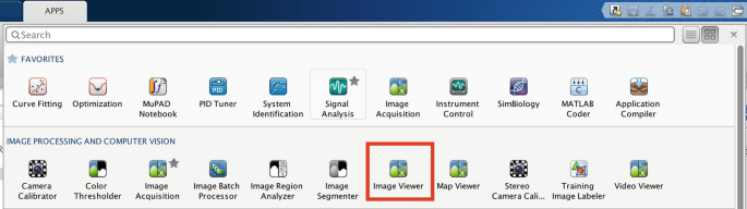
Access to various apps in the tool-strip of MATLAB. The apps accessible will depend on the tool-boxes you have installed
Fig. 5.6 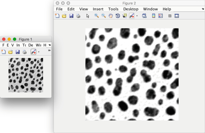
The “blobs” from ImageJ displayed without (left) and with (right) scaling of intensity and size
-
2.
Open the MATLAB app Image Viewer either from the tool-strip or by typing imtool
-
3.
From the Image Viewer go to File > Open ... and select an image
-
4.
Adjust the contrast, inspect the pixels, measure a distance, etc, using the tool-strip shortcuts


5.4.1 Reading and Displaying an Image
This, however, is not much different from what we can do in ImageJ. The real difference comes when we start working from the command-line and making scripts—while this is also possible in ImageJ, it is a lot easier in MATLAB. Assuming you have an image named “blobs.tif” on your desktop, try this
1 >> cd /Users/simon/Desktop 2 >> myBlobs = imread(’blobs.tif’); 3 >> figure (1); clf 4 >> imshow(myBlobs) 5 >> figure (2); clf 6 >> imshow(myBlobs, ’displayrange’, [10 200], ... 7 ’initialmagnification’, ’fit’)
Here is what we just did: (1) We navigated to the directory holding our image; (2) Read the image into the variable myBlobs using the imread command; (3) Selected figure number 1 (or created it if it didn’t exist yet) and cleared it; (4) Displayed the content of our variable myBlobs in figure 1; (5) Selected, or created, figure number 2 and cleared it; (6) Again displayed the content of myBlobs but now with the displayed gray-scale confined (especially relevant for 16bit images that otherwise appear black), and the displayed image fitted to the size of the window.
5.4.2 Extracting Meta-Data from an Image
Because we are becoming serious image-analysts we also take a look at the meta-data that came with the image.
1 >> blobInfo = imfinfo(’blobs.tif’); 2 >> whos blobInfo 3 Name Size Bytes Class Attributes 4 5 blobInfo 1x1 5908 struct 6 7 >> blobInfo 8 9 blobInfo = 10 11 Filename: ’/Users/simon/Desktop/blobs.tif’ 12 FileModDate: ’05-Jun-2016 09:45:04’ 13 FileSize: 65172 14 Format: ’tif’ 15 FormatVersion: [] 16 Width: 256 17 Height: 254 18 BitDepth: 8 19 ColorType: ’grayscale’ 20 FormatSignature: [77 77 0 42] 21 ByteOrder: ’big-endian’ 22 NewSubFileType: 0 23 BitsPerSample: 8 24 Compression: ’Uncompressed’ 25 PhotometricInterpretation: ’WhiteIsZero’ 26 StripOffsets: 148 27 SamplesPerPixel: 1 28 RowsPerStrip: 254 29 StripByteCounts: 65024 30 XResolution: [] 31 YResolution: [] 32 ResolutionUnit: ’Inch’ 33 Colormap: [] 34 PlanarConfiguration: ’Chunky’ 35 TileWidth: [] 36 TileLength: [] 37 TileOffsets: [] 38 TileByteCounts: [] 39 Orientation: 1 40 FillOrder: 1 41 GrayResponseUnit: 0.0100 42 MaxSampleValue: 255 43 MinSampleValue: 0 44 Thresholding: 1 45 Offset: 8 46 ImageDescription: ’ImageJ=1.50b...’
After your experience with ImageJ you should have no problems understanding this information. What is new here, is that the variable blobInfo that we just created is of the type struct. Elements in such variables can be addressed by name, like this:
1 >> blobInfo.Offset 2 3 ans = 4 5 8 6 7 >> blobInfo.Filename 8 9 ans = 10 11 /Users/simon/Desktop/blobs.tif
If you want to add a field, or modify one, it is done like this:
1 >> blobInfo.TodaysWeather = ’rainy, sunny, whatever’ 2 3 blobInfo = 4 5 TodaysWeather: ’rainy, sunny, whatever’
Note, that we are modifying the content of the variable inside of MATLAB—the information in the “blobs.tif” file sitting on your hard-drive was not changed. If you want to save the changes you have made to an image (not including the metadata) you need the command imwrite. If you want to also save the metadata, and generally want more detailed control of your tif-image, you need the Tiff command.
When addressing an element by name, you can reduce typing by hitting the TAB-key after entering blobInfo.—this will display all the field-names in the structure.
It is important to realize that imread will behave different for different image formats. For example, the tiff format used here supports the reading of specific images from a stack via the ’index’ input argument (illustrated below) and extraction of pixel regions via the ’pixelregion’ input argument. The latter is very useful when images are large or many as it can speed up processing not having to read the entire image image into memory. On the other hand, jpeg2000 supports ’pixelregion’ and ’reductionlevel’, but not ’index’.
5.4.3 Reading and Displaying an Image-Stack
Taking one step up in complexity we will now work with a stack of tiff-files instead. These are the steps we will go through
-
1.
Open “MRI Stack (528K)” in ImageJ (File > Open Samples)—or use the copy provided
-
2.
Save the stack to your desktop, or some other place where you can find it (File > Save)
-
3.
Load a single image from the stack into a two-dimensional variable
-
4.
Load multiple images from the stack into a three-dimensional variable
-
5.
Browse through the stack using the implay command
-
6.
Create a montage of all the images using the montage command
After performing the first two steps in ImageJ, we switch to MATLAB to load a single image-plane (we will work in the editor, use Live Script if you feel like it) and display it (see. result in ◘ Fig. 5.7):

slice number 7 from mri-stack.tif
1 %% --- INITIALIZE --- 2 clear variables % clear all variables in the workspace 3 close all % close all figure windows 4 clc % clear the command window 5 cd (’~/Desktop’) % change directory to desktop 6 7 %% --- load single image and display it --- 8 mriImage = imread(’mri-stack.tif’, ’index’, 7); 9 imshow(mriImage)
To build a stack in MATLAB we need the extra argument ’index’ to specify which single image to read and where in the stack to write it, here we chose image number 7:
1 mriStack( : , : , 7 ) = imread(’mri-stack.tif’, ’index’,7);
Next, we load the entire mri-stack one image at a time. This is done by writing into the three-dimensional array (data-cube) mriStack using a for-loop (this concept should already be familiar to you from the ImageJ macro sections). We use the colon-notation to let MATLAB know that it should assign as many rows and columns as necessary to fit the images. We also take advantage of already knowing that there are 27 images.
1 for imageNumber = 1 : 27 2 mriStack(: , : , imageNumber) = imread(’mri-stack.tif’, ’index’, imageNumber); 3 end
We can use the whos command to inspect our variables and the implay command to loop through the stack (command line):
1 >> whos 2 Name Size Bytes Class Attributes 3 4 imageNumber 1x1 8 double 5 mriImage 226x186 42036 uint8 6 mriStack 226x186x27 1134972 uint8 7 >> implay(mriStack)
Finally, we want to create a montage. This requires one additional step because we are working on 3-dimensional single-channel data as opposed to 4-dimensional RGB images (the fourth dimension is color)—the montage command assumes/requires 4D data (that is just how it is):
1 mriStack2 = reshape (mriStack, [226 186 1 27]); 2 map = colormap (’copper’); % or: bone, summer, hot 3 montage(mriStack2, map, ’size’, [3 9])
The reshape command is used to, well, reshape data arrays and here we used it to simply add one more (empty) dimension so that montage will read the data. The result is shown in ◘ Fig. 5.8.

A montage of the 27 images in the MRI stack, arranged as 3 × 9 and displayed with the colormap “copper”
We can again inspect the dimensions and data-types using the whos command, this time with an argument that restricts the result to any variable beginning with mriStack
1 >> whos mriStack* 2 Name Size Bytes Class Attributes 3 4 mriStack 226x186x27 1134972 uint8 5 mriStack2 4-D 1134972 uint8
To get the dimensions of the 4D mristack2 variable we use the command size
1 > size (mriStack2) 2 3 ans = 4 5 226 186 1 27
Here, the third dimension is the color channel.
5.4.4 Smoothing, Thresholding and All That
Yes, of course we can perform all these operations and here is a small taste of how it is done. We are going to
-
1.
Load an image and invert it
-
2.
Create a copy of it that has been smoothed with a Gaussian kernel
-
3.
Determine the Otsu threshold for this copy
-
4.
Create a binary image based on the smoothed copy
-
5.
Display the mask on the original
-
6.
Apply this mask (binary image) to the original and make measurements through it
-
7.
Display measurements directly on the original (inverted) image
In the editor, we first initialize, then load, invert, and display the result:
1 %% --- INITIALIZE --- 2 clear variables 3 close all 4 clc 5 tfs = 16; %title font size 6 7 %% --- load image --- 8 cd ~/Desktop 9 blobs = imread(’blobs.tif’); % read tif 10 blobs_inv = 255 - blobs; %invert 8bit image 11 12 %% --- display the inverted image --- 13 figure (1) 14 imshow(blobs_inv, ’initialmagnification’, ’fit’) 15 title (’Inverted’, ’fontsize’, tfs)
Next, we smooth the inverted image with a Gaussian kernel, detect the Otsu threshold, apply it, and display the result:
1 %% --- Gaussian smooth and Otsu threshold --- 2 blobs_inv_gauss = imgaussfilt(blobs_inv, 2); % sigma = 2 pixels 3 OtsuLevel = graythresh(blobs_inv_gauss); % find threshold 4 blobs_bw = imbinarize(blobs_inv_gauss, OtsuLevel); % apply threshold 5 6 %% --- display the thresholded image --- 7 figure (2) 8 imshow(blobs_bw, ’initialmagnification’, ’fit’) 9 title (’Inverted, Smoothed, Thresholded’, ’fontsize’, tfs)
To illustrate, on the grayscale image, what we have determined as foreground, we mask it with the binary image blobs_bw by multiplying pixel-by-pixel:
1 %% --- mask the inverted image with the thresholded image --- 2 blobs_bw_uint8 = uint8(blobs_bw); % convert logical to integer 3 blobs_masked = blobs_inv .* blobs_bw_uint8; % mask image 4 5 %% --- display the masked image --- 6 figure (3) 7 imshow(blobs_masked, ’initialmagnification’, ’fit’) 8 title (’Inverted and Masked’, ’fontsize’, tfs)
As an alternative to showing the masked image we can choose to show the outlines of the connected components (the detected blobs):
1 %% --- find perimeter of connected components --- 2 blobs_perimeter = bwperim(blobs_bw); % perimeter of white connected components 3 blobs_summed = blobs_inv + 255 * uint8(blobs_perimeter); % convert, scale, and overlay perimeter on image 4 5 %% --- display image with perimeter overlaid --- 6 figure (4) 7 imshow(blobs_summed, ’initialmagnification’, ’fit’) 8 title (’Inverted, Masked, Outlines’, ’fontsize’, tfs)
In step two we convert the logical variable blobs_perimeter to an 8-bit unsigned integer on the fly (and multiplied it by 255 to increase the intensity), before adding it to the image. If you wonder why we do this conversion, just try to omit it and read the error-message from MATLAB.
Now, let’s make some measurements on the b/w image and display them on the blobs_summed image from above:
1 %% --- measure areas etc on b/w image --- 2 stats = regionprops(blobs_bw, ’area’, ’perimeter’, ’centroid’); % extract features from thresholded image 3 centroids = cat(1, stats.Centroid); % reformat the centroid data to array 4 5 %% --- display centroid positions overlaid on grayscale with outlines --- 6 figure (4) % this figure already exists, we are now adding to it 7 hold on % tell MATLAB too keep what is already in the figure 8 plot (centroids(:, 1), centroids(:, 2), ’*r’) % use red asteriks 9 title (’Inverted, Masked, Outlines, Centroids’, ’fontsize’, tfs)
The result of this step is shown in ◘ Fig. 5.9.

“Blobs” shown with outlines of threshold-based segmentation overlaid. The centroid of each connected component is marked with a red asterisk
Finally, we measure the gray-scale image using the masks—this should remind you of the “Redirect to:” option in ImageJ (Analyze > Set Measurements …):
1 %% --- measure grayscale values --- 2 labels = bwlabel(blobs_bw); % get identifier for each blob 3 statsGrayscale = regionprops(labels, blobs_inv, ’meanIntensity’); % measure pixel-mean for each blob 4 meanIntensity = cat(1, statsGrayscale.MeanIntensity); % reformat the extracted date 5 6 %% --- display measurements on image --- 7 % again, we add to an already existing image 8 figure (3); hold on 9 xOffset = 10; % number of pixels to shift the text to the left 10 text (centroids(:, 1) - xOffset, centroids(:, 2), num2str (meanIntensity, 4), ’color’, ’blue’, ’fontsize’, 10)
Here, we subtracted 10 from the x-coordinate to shift the text ten pixels to the left and thereby centering it a bit better on the detected blobs. We also indicate that we want at most four digits displayed.
The result is shown in ◘ Fig. 5.10.

Masked version of “blobs” with the measured mean intensity for each connected component shown
Exercise: Do this and understand each step! The code shown above is available in blobAnalysis.m.
5.5 Time-Series Analysis
MATLAB has a dedicated data type called simply timeseries. We shall not be using this class here as it is too specialized for what we want to do. At a later stage in your research you might find it useful, but be warned that is was developed probably more with the financial sector in mind and may not support quite the kind of analysis you need to perform.
Whether or not you actually have a time-series or simply an ordered list of data often does not matter. Many of the tools are the same but were indeed developed by people doing signal-processing for, e.g., telephone companies, i.e., they worked on actual time-series data.
5.5.1 Simulating a Time-Series of Brownian Motion (Random Walk)
Physical example: Diffusing molecule or bead. A particle undergoing Brownian motion (read Brown’s paper Brown et al. (1828), it is delightful!) is essentially performing a random walk: In one dimension, each step is equally likely to be to the right or left. If, in addition, we make the size of the step follow a Gaussian distribution, we essentially have Brownian motion in one dimension, also known as diffusion. Here, we will simplify a bit and set a number of physically relevant constants to one, just to keep the code simpler.
The code for generating the random numbers goes something like this (see entire script of name simulateAndPlotBrownianMotion.m):
1 %% --- INITIALIZE --- 2 clear variables 3 close all 4 clc 5 6 % --- simulation settings --- 7 dt = 1; % time between recordings 8 t = (0 : 1000) * dt; % time 9 10 %% --- GENERATE RANDOM STEPS --- 11 stepNumber = numel(t); % number of steps to take 12 seed = 42; % "seed" for the random number generator 13 rng(seed); % reset generator to postion "seed" 14 xSteps = randn (1, stepNumber) * sqrt (dt); % Gaussian distributed steps of zero mean
At this stage you do not have to understand the function of the sqrt (dt) command—with dt = 1 it is one anyway—it is here because this is how Brownian motion actually scales with time. The seed variable and the rng command together control the state in which the (pseudo-)random number generator is started—with a fixed value for seed we will always produce the same random numbers (take a moment to ponder the meaning of randomness when combined with a computer).
After this, we calculate the positions of the particle and the experimentally determined speeds (we will return to these in detail below):
1 %% --- CALCULATE POSITIONS AND SPEEDS --- 2 xPos = cumsum (xSteps); % positions of particle 3 varSteps = var(xSteps); % variance of step-distribution 4 5 xVelocity = diff (xPos) / dt; % "velocities" 6 xSpeed = abs (xVelocity); % "speeds" 7 8 meanSpeed = mean (xSpeed); 9 stdSpeed = std (xSpeed); 10 11 %% --- DISPLAY NUMBERS --- 12 disp ([’VAR steps = ’ num2str(varSteps)]) 13 disp ([’Average speed = ’ num2str (meanSpeed)]) 14 disp ([’STD speed = ’ num2str (stdSpeed)])
In the last three lines we used the command disp that displays its argument in the command window. It takes as argument variables of many different formats, incl. numerical and strings. Here, we gave it a string variable that was concatenated from two parts, using the [ and ] operators (other options are to use the commands cat, strcat, or horzcat). The first part is an ordinary string of text in single quotes, the second part is also a string but created from a numeric variable using the command num2str.
The other MATLAB commands cumsum, diff, mean, and std do what they say and calculate the cumulative sum, the difference, the mean, and the standard deviation, respectively. Look up their documentation, using the doc command, for details and additional input arguments.
5.5.2 Plotting a Time-Series
Ok, now let us plot some of these results:
1 %% --- PLOT STEPS VERSUS TIME --- 2 figure ; hold on; clf 3 plot (t, xSteps, ’-’, ’color’, [0.2 0.4 0.8]) 4 xlabel (’Time [AU]’) 5 ylabel (’Step [AU]’) 6 title (’Steps versus time’)
The output of these lines, and a similar pair for the positions, is shown in ◘ Fig. 5.11. See the script simulateAndPlotBrownianMotion.m to learn how to tweak plot parameters.

Steps (left) and positions (right) as a function of time for a one-dimensional random walk
5.5.3 Histograms
Let us now examine the distribution of step-sizes. We do that by plotting a histogram:
1 %% --- PLOT HISTOGRAM OF STEPS --- 2 figure ; hold on 3 binNumber = floor ( sqrt (stepNumber)); 4 histHandle = histogram(xSteps, binNumber) 5 xlabel (’Steps [AU]’) 6 ylabel (’Count’) 7 title (’Histogram of step-sizes’)
◘ Figure 5.12 show the resulting plot. The command histogram was introduced in MATLAB R2014b and replaces the previous command hist—they are largely similar but the new command makes it easier to create pretty figures and uses the color-scheme introduced in MATLAB R2014b: Since version R2014b, MATLAB’s new default colormap is called “parula” and replaces the previous default of “jet”.

Histogram of step sizes for a random walk. The steps were generated with the command randn that creates pseudo-random numbers from a Gaussian distribution
5.5.4 Sub-Sampling a Time-Series (Slicing and Accessing Data)
Sometimes we can get useful information about our time-series by sub-sampling it. An example could be a signal x, that is corrupted by nearest-neighbor correlations: To remove this, simply remove every second data-point, like this:
1 x = 0 : 0.1 : 30; 2 xSubsampled = x(1 : 2 : end );
Or, if you wanted only every third data-point from the first 200 entries:
1 xSubsampled = x(1 : 3 : 200);
What we just illustrated, was how to read only selected entries from a vector; in the first example we read every second entry from the beginning (the first element in a vector in MATLAB has index 1, not 0), in steps of 2, until the end. The same idea holds for arrays of arbitrary dimension in MATLAB; each dimension is treated independently.
If we wanted, we could also have given a list of indices to read, like this:
1 readThese = [2 5 7 88 212]; % data-points to read 2 xSubsampled = x(readThese);
Alternatively, if we only wanted to replace a single element, say in entry 7, with the number 3; or find all entries larger than 0.94, then set them to 1:
1 % --- replace single element --- 2 x(7) = 3; % overwrite/add the 7th element with "3" 3 4 % --- replace several elements --- 5 xIndex = find (x > 0.94); 6 x(xIndex) = 1; % write "1" in positions from xIndex
The find command is very useful for data-wrangling and thresholding. Combined with the query command isNaN (asking if something “is not-a-number”) you will certainly find yourself applying it once working with real-world data.
5.5.5 Investigating How “Speed” Depends on Δt
After having carefully examined the steps and trajectories we may get the idea of also looking into the velocities and their sizes (speeds). Velocities can be calculated from positions by differentiation wrt. time. Since we have a discrete time-series, we do that by forming the difference and dividing by the time-interval Δt—this is what we did above with the help of the diff command.
And this is where it gets interesting: When we vary Δt, our estimate of the speed also changes! Does this make sense? Take a minute to think about it: What we are finding is that, depending on how often we determine the position of a diffusive particle, the estimated speed varies. Would you expect the same behavior for a car or a plane? Ok, if this has you a little confused you actually used to be in good company, that is, until Einstein explained what is really going on, back in 1905—you might know the story.
The take-home message is that speed is ill-defined as a measure for Brownian motion. This is because Brownian motion is a fractal, so, just like when you try to measure the length of Norway’s coast-line, the answer you get depends on how you measure. If you are wondering what we can use instead, read on, the next section, on the mean-squared-displacement, has you covered.
5.5.6 Investigating How “Speed” Depends on Subsampling
Another way of investigating the fractal nature of Brownian motion is to directly subsample the already recorded (simulated) time-series of positions. That is, we create a new time-series from the existing one by only reading every second, or third, or fourth etc. time and position data, and then calculate the speed for this new time-series:
1 %% --- SUBSAMPLE THE POSITIONS --- 2 % --- Re-sample at every fourth time-point --- 3 t_subsampled_4 = t(1 : 4 : end ); 4 xPos_subsampled_4 = xPos(1 : 4 : end ); 5 meanSpeed4 = mean ( abs ( diff (xPos_subsampled_4)/dt/4)); 6 7 % --- Re-sample at every eighth time-point --- 8 t_subsampled_8 = t(1 : 8 : end ); 9 xPos_subsampled_8 = xPos(1 : 8 : end ); 10 meanSpeed8 = mean ( abs ( diff (xPos_subsampled_8)/dt/8));
Notice how we used, hard to read, compact notation by chaining several commands to calculate the mean speed in a single line—this is possible to do, but usually makes the code harder to read.
Let us now plot these new time-series on top of the original
1 %% --- ZOOMED PLOT SUBSAMPLED POSITION VERSUS TIME --- 2 figure ; hold on; 3 plot (t, xPos, ’-k.’, ’markersize’, 16) 4 plot (t_subsampled_4, xPos_subsampled_4, ’--or’, ’markersize’, 6) 5 plot (t_subsampled_8, xPos_subsampled_8, ’:sb’, ’markersize’, 10) 6 legend (’Every position’, ’Every fourth position’, ’Every eighth position’) 7 set ( gca , ’xlim’, [128 152]) 8 9 xlabel (’Time [AU]’) 10 ylabel (’Position [AU]’) 11 title (’Position versus time’)
This code, where we added a few extras such as control of the size of markers, should generate a plot like the one shown in ◘ Fig. 5.13

Position as a function of time for a one-dimensional random walk. Black dots show the original time-series. If we had only recorded this trajectory at 1/4 or 1/8 the sampling frequency we would have found the positions indicated by red circles and blue squares, respectively. If we were to estimate the speed for each of these three time-series we would find that the red trace has half (\( 1\slash \sqrt{4} \)) the speed of the black, and the blue has \( 1\slash \sqrt{8}\simeq 0.35 \) that of the black. Conclusion: The “speed” depends on how often we measure and is therefore clearly an ill-defined parameter for Brownian motion
5.5.7 Simulating Confined Brownian Motion
Brownian motion doesn’t have to be free. The observed particle could be trapped in a small volume or elastically tethered to a fixed point. To be specific, let us choose as physical example a sub-micron sized bead in an optical trap, in water. This turns out to be just as easy to simulate as pure Brownian motion. Writing down the equations of motion and solving them (or using intuition) we see that the observed positions are simply given by random numbers from a Gaussian distribution. The width of the distribution is determined by the strength of the trap (size of the confinement, stiffness of tether). Importantly, we are not sampling the position of this bead very often, only every millisecond or so, rarely enough that it has time to “relax” in the trap between each determination.
1 sampleNumber = 1001; % number of position determinations 2 xTrapped = randn (1, sampleNumber); % position of bead in trap
What do we get if we repeat the above analysis? Try it.
5.5.8 Simulating Directed Motion with Random Tracking Error
We may also want to create a time-series that is a hybrid: We have a particle that moves with constant speed in one direction, but the position determination is contaminated with random tracking errors. The simulation, again, is simple:
1 %% --- INITIALIZE --- 2 dt = 1; % time between recordings 3 t = 0 : dt : 1000 * dt; % time 4 v = 7; % constant translation speed 5 6 %% --- GENERATE POSITIONS --- 7 xPos = v*t + randn (1, sampleNumber); % position of bead in trap
Repeat the above analysis for this new time-series. How does the speed determination depend on the degree of smoothing, sub-sampling, or Δt? Here, the concept of speed does make sense, and averaging over time (smoothing) should give a better determination, see ► Sect. 5.5.10.
5.5.9 Loading Tracking Data from a File
Instead of analyzing simulated data we often want to work on actual experimental data. If your data was generated in ImageJ with the TrackMate plugin, the output (when exporting tracks) would be an XML file and we would need a parser (reader) for it called importtrackmatetracks.m in order to get the data into MATLAB. See introduction here and code here. This function will return a cell-array of tracks consisting of time, x, y, and z positions (the concept of a function is explained below in ► Sect. 5.6.1.1):
1 function [tracks, metadata] = importTrackMateTracks(file, clipz, scalet) 2 %%IMPORTTRACKMATETRACKS Import linear tracks from TrackMate 3 % 4 % This function reads a XML file that contains linear tracks generated by 5 % TrackMate (http://fiji.sc/TrackMate). Careful: it does not open the XML 6 % TrackMate session file, but the track file exported in TrackMate using 7 % the action ’Export tracks to XML file’. This file format contains less 8 % information than the whole session file, but is enough for linear tracks 9 % (tracks that do not branch nor fuse). 10 % 11 % SYNTAX 12 % 13 % tracks = IMPORTTRACKMATETRACKS(file) opens the track file ’file’ and 14 % returns the tracks in the variable ’tracks’. ’tracks’ is a cell array, 15 % one cell per track. Each cell is made of 4xN double array, where N is the 16 % number of spots in the track. The double array is organized as follow: 17 % [Ti, Xi, Yi, Zi ; ...] where T is the index of the frame the spot has been 18 % detected in. T is always an integer. X, Y, Z are the spot spatial 19 % coordinates in physical units. 20 . 21 . 22 .
To get a feeling for the data: Pick a few individual tracks and submit them to the same analysis as above. Try a few from the different experimental conditions (try both long and short tracks). Do you notice any difference?
5.5.10 Smoothing (Filtering) a Time-Series
If you suspect that some of the jitter in your signal is simply noise, you can smooth the signal. This is very much the same procedure as when smoothing an image. The relevant command is smooth (requires the Curve Fitting Toolbox) and it has several options for adaptation to your needs:
1 % --- simple smoothing --- 2 xPosSmoothed = smooth(xPos); % defaults to moving average over 5 data points 3 4 % --- sophisticated smoothing --- 5 span = 7; % number of data points to average over 6 method = ’sgolay’ ; % Savitsky-Golay filter 7 degree = 3; % the order of the s-g filter 8 9 xPosSmoothed = smooth(xPos, span, method, degree);
5.6 MSD: Mean Square Displacement
Motivated by the shortcomings of the speed as a measure for motion, we try our hands at another measure. This measure, while a bit more involved, does not suffer the same problems as the speed but takes a little getting used to. Without further ado:
The mean square displacement for a one-dimensional time-series x(t), sampled continuously, is defined as
where 〈⋅〉 is the expectation value of the content, either in the ensemble sense or with respect to t (same thing if the system is ergodic)—think of it as the average over all time-points. It measures how far a particle has moved, in an average sense, in a time-interval of size τ.
In practice, we need to replace the expectation-value-operation 〈⋅〉, with something we can calculate based on our data. There are several ways of doing this, see Qian et al. (1991), and the following is one of the more popular and meaningful ones, for time-lag τ = k Δt:
where M is the number of postion-determinations of x. Please note, that we are averaging over the track itself using a sliding window: This means that our estimates for the MSD are not independent for consecutive values of the time-lag τ—this is the price we pay for reducing noise and using all the data.
◘ Figure 5.14 shows theoretical and simulated results for the MSD for three different types of motion: (1) Brownian motion (free diffusion); (2) Brownian motion in an optical trap (confined diffusion); and (3) Random motion with finite persistence (Ornstein-Uhlenbeck process)

Mean-squared displacement for the Ornstein-Uhlenbeck process (persistent random motion), Brownian motion in an optical trap (confined diffusion), and Brownian-motion proper (free diffusion). Straight lines show slopes of one (green) and two (blue), for comparison to the cases of Brownian motion and linear motion. Green points: Freely diffusing massless particle (Einstein’s Brownian motion); red points: trapped massless particle (OT limit, or OU velocity process); and blue points: freely diffusing massive particles (time integral of OU process). This is ◘ Fig. 8 in Nørrelykke and Flyvbjerg (2011)
5.6.1 Creating a Function That Calculates MSDs
One of the great thing about the MSD is that there are no approximations when moving from continuous to discrete time: There are no sampling artifacts. For a fixed time-lag, the MSD can be calculate in MATLAB by defining a function like this:
1 function msd_tau = fun_msd_at_tau_1dim(x,tau) 2 3 % fun_msd_at_tau_1dim FUNCTION 4 % GIVEN INPUT DATA ’X’ THIS FUNCTION RETURNS THE 5 % MEAN-SQUARED-DISPLACEMENT CALCULALTED IN OVERLAPPING WINDOWS 6 % FOR THE FIXED TIMELAG VALUE ’tau’ 7 % NB: THIS IS FOR A SINGLE TIMELAG ONLY BUT AVERAGED OVER THE ENTIRE TRACK 8 9 % 2016-06-03, sfn, created 10 % 2016-06-10, sfn, modified for one dimension 11 % 2017-05-15, sfn, nomenclature changes 12 13 %% --- INITIALIZE --- 14 M = length (x); % number of postions determined 15 dr2 = zeros (1, M - tau); % initialize and speed up procedure 16 17 %% --- CALCULATE THE MSD AT A SINGLE TIMELAG --- 18 for k = 1 : M - tau 19 dx2 = (x(k + tau) - x(k)).^2; % squared x-displacement 20 21 dr2(k) = dx2; % store the squared x-displacement for each postion of the sliding window 22 end 23 24 msd_tau = mean (dr2); % The mean of the squared displacements calculated in sliding windows
In this code-example you should notice that we declared a function, used the command zeros to pre-allocate memory hence speed up the procedure, and squared each element in a vector with the .̂ operator which should not be confused with the ̂ operator that would have attempted to form the inner product of the vector with itself (and fail). If your function-call fails, you might have to tell MATLAB where to find the function using the addpath command or by clicking on “set path” in the HOME tab and then pointing to the folder that holds the function.
5.6.1.1 About Functions and How to Call Them
A function is much like a normal script except that it is blind and mute: I doesn’t see the variables in your workspace and whatever variables are defined inside of the function are not visible from the workspace either. One way to get data into the function is to feed it explicitly as input, here as x and tau. The only data that gets out is that explicitly stated as output, here msd_tau. This is how you call the function msd_tau, ask it to calculate the mean square displacement for the time-series with coordinates (x, y), for a single time-lag of τ = 13 and return the result in the variable dummy:
1 >> dummy = fun_msd_at_tau_1dim(x, 13);
Having learnt how to do this for a single time-lag, we can now calculate the MSD for a range of time-lags using a for loop:
1 for tau = 1 : 10 2 msd(tau) = fun_msd_at_tau_1dim(x, tau); 3 end
After which we will have a vector of length ten holding the MSD for time-lags one through ten. If the physical time-units are non-integers you simply plot MSD against these, do not try to address non-integer positions in a vector or matrix, they do not exist. This will become clear the first time you try it.
To build some further intuition for how the MSD behaves, let us calculate it analytically for a couple of typical motion patterns.
5.6.2 MSD: Linear Motion
By linear motion we mean
where v is a constant velocity and t is time. That is, the particle was at position zero at time zero, x(t = 0) = 0, and moves to the right with constant speed. The MSD then becomes
i.e., the MSD grows with the square of the time-lag τ. In a double-logarithmic (log-log) plot, the MSD would show as a straight line of slope 2 when plotted against the time-lag τ:
5.6.3 MSD: Brownian Motion
By Brownian motion we mean
where \( \dot{\mkern6mu} \) means differentiation wrt. time, \( a=\sqrt{2D} \), D is the diffusion coefficient and η is a normalised, Gaussian distributed, white noise
where δ is Dirac’s delta function. See Wikipedia for an animation of Brownian motion:
► https://en.wikipedia.org/wiki/Brownian_motion
With this equation of motion we can again directly calculate the MSD:
a result that should be familiar to some of you.
Apart from prefactors, that we do not care about here, the crucial difference is that the MSD now grows linearly with the time-lag τ, and in a log-log plot it would hence be a straight line with slope one when plotted against τ.
We are much more interested in the mathematical properties of this motion than in the actual thermal self-diffusion coefficient D: The temporal dynamics of this equation can be used to model systems that move randomly, even if not driven by thermal agitation. So, when we say Brownian motion, from now on, we mean the mathematical definition, not the physical phenomenon.
For those interested in some mathematical details, Brownian motion can be described via the Wiener process W, with the white noise being the time-derivative of the Wiener process \( \eta =\dot{W} \). The Wiener process is a continuous-time stochastic process and is one of the best known examples of the broader class of Levý processes that can have some very interesting characteristics such as infinite variance and power-law distributed step-sizes. These processes come up naturally in the study of the field of distributions, something you can think of as being a generalization of ordinary mathematical functions, and also requires an extension of normal calculus to what is known as Itô calculus. If you are into mathematical finance or stochastic differential equations you will know all of this already.
5.6.3.1 MSD: Simulated Random Walk
We can also calculate the MSD for the discrete random walk that we simulated earlier. There, we simplified our notation by setting 2D = 1 but otherwise the random walk was a mathematically exact representation of one-dimensional free diffusion. Here is the calculation, for a time-lag of τ = k Δt and explicitly including the \( \sqrt{2D} \) prefactor; you should already have all the ingredients to understand each step:
here we used that the position at time n Δt is the sum of the steps before then:
where ζ are Gaussian distributed random numbers of zero mean, unit variance, and uncorrelated:
with δ i,j Kronecker’s delta: Zero for i and j different, unity if they are the same. These ζ-values are the ones we created with the randn command in MATLAB. Again, we see that the MSD is linear in the time-lag τ = k Δt.
5.6.4 MSD: Averaged Over Several 2-Dim Tracks
To start quantifying the motion of multiple tracks, in two spatial dimensions, we first calculate the mean-squared-displacement for an individual track m
where k = 1, 2, …, M m − 1 is the time-lag in units of Δt and M m is the number of positions determined for track m. Notice, that we use a sliding window so that the M m − k determinations of the MSDs at time-lag k Δt are not independent; this introduces strong correlations between the MSD calculated at neighboring time-lags by trading independence for smaller error-bars Wang et al. (2007).
One way to calculate the sample-averaged MSD is to weigh each MSD by the number of data-points used to calculated it
where the sums extend over all time-series with M m > k. Here, the weights are chosen as equal to the number of intervals that was used to calculate the MSD for a given time-lag and track.
5.6.5 Further Reading About Diffusion, the MSD, and Fitting Power-Laws
Papers dealing with calculation of the MSD: Qian et al. (1991) and under conditions with noise: Michalet (2010). Analytically exact expressions for several generic dynamics cases (free diffusion, confined diffusion, persistent motion both free and confined): Nørrelykke and Flyvbjerg (2011). Determining diffusion coefficients when this or that moves or not, this is an entire PhD thesis compressed to one long paper: Vestergaard et al. (2014). How to fit a power-law correctly and what can happen if you do it wrong like most people do—an absolute must-read: Clauset et al. (2009).
Take Home Message
Ok, good, you made it to here. Congratulations!
If this was your first encounter with coding, MATLAB, or numerical simulations you may feel a bit overwhelmed at this point—don’t worry, coding isn’t mastered in one day; put in the hours and you will learn to master MATLAB, like many have before you. If you already knew MATLAB you probably skipped this chapter.
Here is what you just learned how to do in MATLAB:
-
Create a plot and save it to a file in pdf, png, or other formats
-
Load an image and process it (smoothing, thresholding)
-
Perform measurements on an image and overlay those measurements on the image
-
Read and modify the meta-data in an image file
-
Simulate a random walk as a model for free diffusion (Brownian motion), confined/tethered motion, and directed motion with tracking error
-
Calculate and display the mean square displacement (MSD)—a robust measure of motion
-
Spot when “speed” is a flawed measure for motion (the mean will depend on the sampling interval)—when there is a random component, it is always a flawed measure
-
Structure and document your code, keeping good code hygiene
Notes
- 1.
By now, you have probably noticed that some words are typeset like this. Those are words that MATLAB recognize as commands (excluding commands that are specific to toolboxes).
Bibliography
Brown R, Hon FRS, MRSE, Acad RI, VPLS (1828) XXVII. A brief account of microscopical observations made in the months of June, July and August 1827, on the particles contained in the pollen of plants; and on the general existence of active molecules in organic and inorganic bodies. Philos Mag 4(21):161–173. https://doi.org/10.1080/14786442808674769
Clauset A, Shalizi CR, Newman MEJ (2009) Power-law distributions in empirical data. SIAM Rev 51(4):661–703
Michalet X (2010) Mean square displacement analysis of single-particle trajectories with localization error: Brownian motion in an isotropic medium. Phys Rev E Stat Nonlin Soft Matter Phys
Nørrelykke SF, Flyvbjerg H (2011) Harmonic oscillator in heat bath: exact simulation of time-lapse-recorded data and exact analytical benchmark statistics. Phys Rev E Stat Nonlin Soft Matter Phys 83(4):041103
Qian H, Sheetz MP, Elson EL (1991) Single particle tracking. Analysis of diffusion and flow in two-dimensional systems. Biophys J 60(4):910–921
Vestergaard C, Blainey PC, Flyvbjerg H (2014) Optimal estimation of diffusion coefficients from single-particle trajectories. Phys Rev E Stat Nonlin Soft Matter Physics
Wang YM, Flyvbjerg H, Cox EC, Austin RH (2007) When is a distribution not a distribution, and why would you care: single-molecule measurements of repressor protein 1-D diffusion on DNA. In: Controlled nanoscale motion: nobel symposium, vol 131, pp 217–240. Springer, Berlin/Heidelberg. ISBN: 978-3-540-49522-2. https://doi.org/10.1007/3-540-49522-3_11
Acknowledgements
We thank Ulrike Schulze (Wolfson Imaging Centre–MRC Weatherall Institute of Molecular Medicine, Micron Oxford Advanced Bioimaging Unit, University of Oxford) for reviewing this chapter.
Author information
Authors and Affiliations
Corresponding author
Editor information
Editors and Affiliations
Appendices
Appendix: MATLAB Fundamental Data Classes
All data stored in MATLAB has an associated class. Some of these classes have obvious names and meanings while others are more involved, e.g. the number 12 is an integer, whereas the number 12.345 is not (it is a double), and the data-set {12, 'Einstein', 7+6i, [1 2 ; 3 4]} is of the class cell. A short video (5min) about MATLAB fundamental classes and data types.
Here are some of the classes that we will be using, sometimes without needing to know it, and some that we won’t:
- single, double :
-
32 and 64 bit floating number, e.g. 1’234.567 or -0.000001234. The default is double.
- int8/16/32/64, uint8/16/32/64 :
-
(unsigned-)integers of 8/16/32/64 bit size, e.g. -2 or 127
- logical :
-
Boolean/binary values. Possible values are TRUE, FALSE shown as 1,0
- char :
-
characters and strings (largely the same thing), e.g. ’hello world!’. Character arrays are possible (all rows must be of equal length) and are different from cell arrays of characters.
- cell :
-
cell arrays. For storing heterogeneous data of varying types and sizes. Very flexible. Great potential for confusion. You can have cells nested within cells, nested within cells …
- struct :
-
structure arrays. Like cell arrays but with names and more structure; almost like a spreadsheet.
- table :
-
tables of heterogeneous but tabular data: Columns must have the same number of rows. Think “spreadsheet”. Supports useful commands such as summary. New data format from 2013b.
- categorical :
-
categorical data such as ’Good’, ’Bad’, ’Horrible’, i.e., data that take on a discrete set of possible values. Plays well with table. New data format from 2013b.
5.1.1 MATLAB Documentation Keywords for Data Classes
The following is a list of search terms related to the cell, struct, and table data classes. They are titles of individual help-documents and are provided here because the documentation of MATLAB is vast and it can take some time to find the relevant pages. Simply copy and paste the lines into MATLAB’s help browser in the program or on the web
Access Data in a Cell Array Cell Arrays of Character Vectors Multilevel Indexing to Access Parts of Cells Access Data in a Structure Array Cell vs. Struct Arrays Create and Work with Tables Access Data in a Table
Here is a link to a video about tables and categorical arrays.
Appendix: Do I Have That Toolbox?
To find out which toolbox a particular command requires simply search for it in the documentation and notice the path. Alternatively, use the which command:
1 >> which (’graythresh’) 2 /Applications/MATLAB_R2015b.app/toolbox/images/images/graythresh.m
Any path to a function, as found with the which command, that includes .../toolbox/matlab/... does not require a specific toolbox as it is part of the core MATLAB distribution. It is also possible to use the matlab.codetools.requiredFilesAndProducts command:
1 >> [fileList,productList] = matlab.codetools.requiredFilesAndProducts( ’graythresh’); 2 >> productList.Name 3 4 ans = 5 MATLAB 6 7 ans = 8 Image Processing Toolbox
To find out which toolboxes you have installed, say doc to start the help-browser and click “All Products”, see ◘ Fig. 5.15.

Truncated view of Help window showing “All Products” which includes all the toolboxes you have installed—if it doesn’t say “toolbox” it is something else
Alternatively, navigate to the folder where MATLAB is installed, via command line or MATLAB or Finder. Example for an installation on a Mac, getting the list in iTerm (bash):
1 [simon@SimonProRetina ~]$ ls -lho /Applications/MATLAB_R2015b.app/toolbox/ | head 2 total 0 3 drwxr-xr-x 5 simon 170B Oct 13 2015 aero 4 drwxr-xr-x 7 simon 238B Oct 13 2015 aeroblks 5 drwxr-xr-x 12 simon 408B Oct 13 2015 bioinfo 6 drwxr-xr-x 23 simon 782B Oct 13 2015 coder 7 drwxr-xr-x 11 simon 374B Oct 13 2015 comm 8 drwxr-xr-x 40 simon 1.3K Oct 13 2015 compiler 9 drwxr-xr-x 8 simon 272B Oct 13 2015 compiler_sdk 10 drwxr-xr-x 8 simon 272B Oct 13 2015 control 11 drwxr-xr-x 8 simon 272B Oct 13 2015 curvefit 12 [simon@SimonProRetina ~]$
Here, you need to be able to recognize that the toolbox names are abbreviated, so that, e.g., the Aerospace Toolbox is referred to simply as aero.
Appendix: HTML and Live Scripts
5.1.1 Publish Your Script to HTML
If you want to show your code and it’s output to someone, without running MATLAB, you can do it with the PUBLISH feature. Running this command on your script will execute it and create a folder called “html” in the same place as your script. Inside of this folder you will find a single .html file and perhaps a number of .png files for the figures that your script created. ◘ Figure 5.16 shows the result of publishing to HTML the same code as was shown in ◘ Fig. 5.4.

Example of publishing code to HTML. This is the same code as in the m-script shown in ◘ Fig. 5.4. Notice how the output of the script is included with the code. This is an HTML file and therefor easy to share, but you cannot execute it in MATLAB
5.1.2 Working with Live Scripts
Live Script is a new feature in MATLAB R2016a. You can think of it as something in between publishing to HTML and working directly in the script editor. Existing scripts can be converted to live scripts and the other way around! ◘ Figure 5.17 shows the same code as in ◘ Fig. 5.4, but converted to the live script format (extension mlx). If you have seen iPython notebooks or Mathematica you might see what the inspiration is. Try it out, you might like it! Just keep in mind that it is a new feature and that you cannot share your live-scripts with anyone using an older version than R2016a (unless you convert to standard m-file first).

Example of Live Script, a new feature in MATLAB R2016a. This is the same code as in the m-script shown in ◘ Fig. 5.4. Notice how the output of the script is included with the code. This script can be edited and executed in MATLAB
Appendix: Getting File and Folder Names Automatically
5.1.1 Read from a Folder
To get a list of files in a folder you have several options: (1) Navigate MATLAB to the folder (by clicking or using the cd command) and type ls or dir; (2) Give the ls or dir command followed by the path to the folder, like this
1 >> ls /Users/simon/Desktop/ 2 blobs.tif mri-stack.tif 3 4 >> dir /Users/simon/Desktop/ 5 6 . blobs.tif 7 .. mri-stack.tif
We can also assign the output to variables:
1 >> lsList = ls (’/Users/simon/Desktop/’); 2 >> dirList = dir (’/Users/simon/Desktop/’);
What is the difference between the two variables dirList and lsList?
5.1.2 Path and File Names
To illustrate how to work with and combine file-names and path-names we will introduce the dialogue window (again assuming we are in the /Users/simon/Desktop/ directory and have a file called “blobs.tif” there):
1 >> fileName = uigetfile (’.tif’)
In response to which we should see a dialogue window similar to ◘ Fig. 5.18.

The dialogue window, in OS X, that appears in response to the uigetfile command
We should also be told the name of the file we selected:
1 fileName = 2 3 blobs.tif
If we want more information, such as the location of the file we do:
1 >> [fileName, pathName] = uigetfile (’.tif’) 2 3 fileName = 4 5 blobs.tif 6 7 pathName = 8 9 /Users/simon/Desktop/
From the file- and path-name we can now create the full file-name, incl. the path, using the command fullfile:
1 >> fullFileName = fullfile(pathName, fileName) 2 3 fullFileName = 4 5 /Users/simon/Desktop/blobs.tif
Obviously, if you are working on a different system you file-separator might look different. However, that is because fullfile inserts platform-dependent file separators. If you want more control over this aspect you should look into the filesep command.
Reversely, if you had the full name of a file and wanted to extract the file-name or the path-name, you could do this:
1 >> [pathstr,name,ext] = fileparts(fullFileName) 2 3 pathstr = 4 5 /Users/simon/Desktop 6 7 name = 8 9 blobs 10 11 ext = 12 13 .tif
Alternatively, if all we wanted was the name of a directory we would use the command uigetdir—you can guess what it does.
Why did we just do all this? We did it because we often have to spend a lot of time on data-wrangling before we can even get to the actual data-analysis. Knowing how to easily extract file and path names for your data allows you automate many later steps. Example: You might want to open each image in a directory, crop it, scale it, smooth it, then save the results to another directory with each modified image given the same name as the original but with “_modified” appended to the name.
Appendix: Codehygiene
It is important for your future self, not to mention collaborators, that you keep good practices when coding.
-
The actual code should be easy to read, not necessarily as compact as possible
-
Use descriptive names
-
Document the code
-
Insert plenty of blank spaces: Let your code breathe!
◘ Figure 5.19 is and example of how your code could look, when folded, if you take care to structure it nicely—notice how easy it to figure out what goes on where, without having to read a single line of actual code.

Screenshot of code that is clearly structured and folded. The currently active code-block is highlighted in yellow
Appendix: MATLAB Cheat Sheet
Here are two compact pages that you are encouraged to print separately and keep around when using MATLAB—at least initially. They outline most of the syntax and also list the most commonly used commands. This version (you can find several online) was compiled by Thor Nielsen (thorpn86@gmail.com) ► http://www.econ.ku.dk/pajhede/.


Rights and permissions
Open Access This chapter is licensed under the terms of the Creative Commons Attribution 4.0 International License (http://creativecommons.org/licenses/by/4.0/), which permits use, sharing, adaptation, distribution and reproduction in any medium or format, as long as you give appropriate credit to the original author(s) and the source, provide a link to the Creative Commons license and indicate if changes were made.
The images or other third party material in this chapter are included in the chapter's Creative Commons license, unless indicated otherwise in a credit line to the material. If material is not included in the chapter's Creative Commons license and your intended use is not permitted by statutory regulation or exceeds the permitted use, you will need to obtain permission directly from the copyright holder.
Copyright information
© 2020 The Author(s)
About this chapter

Cite this chapter
Nørrelykke, S.F. (2020). Introduction to MATLAB. In: Miura, K., Sladoje, N. (eds) Bioimage Data Analysis Workflows. Learning Materials in Biosciences. Springer, Cham. https://doi.org/10.1007/978-3-030-22386-1_5
Download citation
DOI: https://doi.org/10.1007/978-3-030-22386-1_5
Published:
Publisher Name: Springer, Cham
Print ISBN: 978-3-030-22385-4
Online ISBN: 978-3-030-22386-1
eBook Packages: Biomedical and Life SciencesBiomedical and Life Sciences (R0)