
Abstract
Overtaking accidents caused by improper operations performed by a driver occur frequently. However, most studies on overtaking safety have neglected research into driver control input. A novel method is proposed to obtain the driver control input during the overtaking process. Meanwhile, to improve the safety of overtaking, two types of safe distances, and the time of the overtaking are considered. Path constraints are established when considering the two types of safe distances. An optimal control model is established to solve the minimum time maneuver under multiple constraints. Using the Gauss pseudospectral method, the optimal control problem is converted into a nonlinear programming problem, which is then solved through sequential quadratic programming (SQP). In addition, the effectiveness of the proposed method is verified based on the results of a Carsim simulation. The simulation results show that by adopting an inverse dynamics method to solve the manipulation problem of the vehicle’s minimum overtaking time, the manipulation capability of a vehicle in completing an overtaking safely within the minimum time can be obtained. This method can provide a reference for research into the active safety of manned and unmanned vehicles.
1 Introduction
With continuous improvements in traffic conditions, vehicles have entered a high-speed era. It is thus necessary to solve the “minimum time problem” in vehicle handling dynamics to satisfy the stability, safety, maneuverability, and high-speed characteristics of a vehicle. With the aim of eliminating the restrictions of slow vehicles or other factors such as road structures, high-speed vehicles will choose when to change lanes to obtain a better driving environment or achieve the desired driving purposes.
The driver’s control input will be affected by the driver’s subjective feelings, previewing time, reaction time, and other uncertain factors, which lead to a lack of uniform and accurate mathematical models in the study of closed-loop systems [1,2,3,4,5]. The study of inverse dynamics in vehicle handling is in contrast to the positive problem. When setting up a model without a driver, the driver’s input can be obtained if the model of the vehicle and the motion state are known [6, 7]. This method is able to compare the maneuverability of different vehicles operated in the most efficient manner. The specified maneuverability involves accurately reaching a given state variable [8, 9], tracking a given path accurately [10,11,12], and passing through the given path within the shortest time without deviating from the given path boundary [13, 14]. The latter situation is the issue studied in this research.
Bernard et al. [15, 16] presented a nonlinear inverse model of a vehicle that simulates combined steering and braking/driving, the results of which show that the inverse method is useful in solving the problem of path tracking under different braking/driving scenarios. Their model has provided a new idea regarding the development and application of vehicle handling dynamics. Fujioka et al. [17] used a transient vehicle dynamics model to represent a vehicle with different driving and steering configurations, and a conjugate gradient descent method was used to solve the minimum time handling problem in which the starting point, ending point, and trajectory are not constrained. However, this will not occur so universally in general application. Hendriks et al. [18] studied the optimal handling inverse problem by applying an optimal control theory and Pontryagin’s minimum principle, the results of which show that different vehicle configurations have different optimal control strategies, and their method can be used to evaluate the optimal transient handling performance of a vehicle. Their algorithm is rather robust with respect to inaccurate starting values, but is the least efficient in terms of speed of convergence. Casanova et al. [19, 20] established a vehicle steering control model based on the linear optimal discrete time preview control theory, and obtained the control input and optimal completion time using an inverse dynamics method. Andreasson et al. [21, 22] used the inverse dynamics method to study the vehicle chassis control, the results of which show that the method is effective for dealing with the complex problems of chassis control. Boyer et al. [23] used a handling inverse dynamics method to study the multi-body dynamics of a vehicle and analyzed its maneuverability. Wang et al. [24] used a multiple shooting method to study the emergency collision avoidance problem. However, the linearization applied in this method makes the quadratic programming problem deviate significantly from the original model. Liu et al. [25,26,27] used the Gauss pseudospectral method to study the optimal path tracking control problem. Their method shows many advantages compared to previous traditional methods. However, all research in this regard was based on the assumption that obstacles are stationary, and dynamic obstacles were not considered.
In summary, the above studies did not involve the minimum time handling problem while overtaking in a dynamic environment, that is, the lateral and longitudinal safety distances in the minimum time handling problem while overtaking were not considered. The longitudinal safety distance refers to the idea that the overtaking vehicle should keep a certain distance with the overtaken vehicle during the overtaking process, thereby avoiding traffic accidents such as a rear-end collision. The lateral safety distance refers to the lateral lane constraint, as well as the constraint of the vehicle width variation caused by a roll. The lateral safety distance is used to ensure the vehicle completes the overtaking behavior only within its own lane and the left adjacent lane; this can avoid the scraping of two vehicles owing to variations in body width. Therefore, considering the influence of the longitudinal and lateral safety distances, with the aim of overtaking the front vehicle as quickly as possible, the optimal overtaking trajectory and the shortest overtaking time are figured out using the inverse dynamics method.
2 Vehicle Motion Model
2.1 3-Degree of Freedom Vehicle Model
Assuming that the tire cornering properties are within the linear range, the vehicle steering motion model is simplified as a 3-degree of freedom (DOF) linear vehicle model with lateral motion, yawing motion, and longitudinal motion, as depicted in Figure 1, where the differential equations of motion are expressed as follows:
where \( v \) is the lateral velocity; \( u \) is the longitudinal velocity; \( \omega_{\text{r}} \) is the yaw rate of the vehicle; \( m \) is the total mass of the vehicle; \( I_{\text{z}} \) is the moment of inertia around the vertical axis; a, b are the distances from the center of the mass to the front and rear axles, respectively; \( k_{1} , \, k_{2} \) are the comprehensive cornering stiffness of the front and rear wheels, respectively; \( \delta \) is the steering angle of the front wheel; \( F_{\text{yf}} \) is the cornering force of the front wheel; \( F_{\text{yr}} \) is the cornering force of the rear wheel; \(F_{\rm{xf}} \) is the driving/braking force of the front wheel (when \(F_{\rm{xf}} \) ≥ 0, \(F_{\rm{xf}} \) is the driving force, and when \(F_{\rm{xf}} \) < 0, \(F_{\rm{xf}} \) is the braking force); \( F_{\text{xr}} \) is the driving/braking force of the rear wheel; \( F_{\text{f}} \) is the rolling resistance (\( F_{\text{f}} = mgf \), where f is the coefficient of the rolling resistance); and \( F_{\text{w}} \) is the air resistance (\( F_{\text{w}} = C_{\text{D}} A(3.6u)^{2} /21.15 \), where \( C_{\text{D}} \) is coefficient of air resistance and A is frontal area).

3-DOF vehicle model
Considering the influence of the driving/braking force, the lateral forces of the front and rear wheels are
where \( \varphi \) is friction coefficient of the road surface, and \( F_{\text{zf}} \) and \( F_{\text{zr}} \) are the vertical forces of the front and rear wheels, respectively.
Considering the longitudinal load transfer, the vertical forces of the front and rear wheels are
where \( h_{\text{g}} \) is the height of vehicle’s center of mass.
To simulate the trajectory of the vehicle, we established a ground reference coordinate system (Figure 1). Letting the coordinates of the vehicle’s center of mass in the \( xoy \) coordinate system be x, y, and the angle between the x’ axis of the vehicle coordinate system and the x axis of the ground reference coordinate system be θ, the vehicle velocity in the ground reference coordinate is projected as
2.2 Vehicle Overtaking Model Based on Two Kinds of Safe Distances
Overtaking is a common phenomenon in the process of vehicle driving. Inappropriate timing of an overtaking, or operational errors, can lead to traffic accidents. In this paper, the entire overtaking process is divided into three phases: lane changing, overtaking, and merging. Taking safety as the premise, aiming at overtaking the vehicle ahead as quickly as possible, and considering the safety distance and relationship between the overtaking and overtaken vehicles during the overtaking process, a new vehicle-overtaking model is established to provide judgment and support.
In this paper, the simulated scenarios of a vehicle overtaking are simplified as follows:
-
(1)
The driving sections are assumed to be straight and flat roads within the city.
-
(2)
There is only one overtaken vehicle, as shown in Figure 2, and vehicles A and B are in the same lane, with no other vehicles in the adjacent lane.
Figure 2 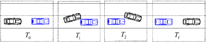
Process for minimum overtaking time
-
(3)
Vehicle B is in front of vehicle A.
-
(4)
Vehicle B drives straight ahead with a uniform velocity, while vehicle A overtakes B with a uniform velocity.

The vehicle should keep a certain distance, which is the safety distance of vehicle A, with the vehicle ahead during the overtaking to avoid a rear-end collision during a lane change. In addition, the safety distance, which is now the safety distance of vehicle B, should still be maintained after the overtaking is achieved. In view of driving safety, the normal overtaking process is as follows: when the distance between the front and rear vehicles is in the longitudinal safety distance, vehicle B can start overtaking, and enters the original lane when the longitudinal distance is at least greater than the safety distance, as shown in Figure 2. Here, T0 is the initial time of the overtaking, Tf is the terminal time of the overtaking, \( D_{\text{a}} \) is the longitudinal safety distance when vehicle A is ahead of vehicle B, and \( D_{\text{b}} \) is the longitudinal safety distance when vehicle B is ahead of vehicle A. The estimated time spent on overtaking is shown in the following:
where \( u_{1} \) and \( u_{0} \) are the speed of vehicles A and B, respectively. The estimated driving distance of vehicle A in this process is \( S_{1} = u_{1} t \), the longitudinal safety distance of the two vehicles is \( D_{\text{a}} \), and the minimum distance for overtaking is \( D_{\text{b}} \).
The 15th item in the “Measures for the Administration of Expressway Traffic,” published by the Chinese government in March of 1995, stipulates that, “When driving a vehicle on a highway, it is necessary to maintain a sufficient distance between the vehicle and the vehicle ahead which are in the same lane. Under normal conditions, when the driving speed is at 100 km/h, the distance headway should be 100 m or more, and when traveling at a speed of 70 km/h, the distance headway should be at least 70 m.” In this paper, the speeds of the overtaking vehicle are 120 and 160 km/h, respectively. In addition, the speed of the overtaken vehicle is 80 km/h, and thus the safety distances are Da1 = 120 m, Da2 = 160 m, and Db = 80 m.
The side-slip angle of the vehicle will change when steering, resulting in a change in the width of the vehicle, the variable quality of which is \( \Delta L = h_{\text{x}} \,{\text{sin}}\,\phi \), where \( h_{\text{x}} \) is the height of the spring. In addition, the direction of the side-slip angle will also change during this process. In order to ensure that no collisions will occur during the overtaking process, assuming that the vehicle’s body width is \( L_{\text{o}} = L + 2h_{\text{x}}\, {\text{sin}}\,\phi_{\text{m}} \) during the overtaking, where L is the body width of the vehicle when driving straight, and \( \phi_{\text{m}} \) is the maximum slip angle when no rollover occurs, \( h_{\text{x}} {\text{sin}}\,\phi_{\text{m}} \) is thus considered to be the lateral safety distance in this study.
2.3 Optimal Control Model
Optimal control is a method that uses a control law to make sure the controlled object can reach a certain required terminal state from the initial state, and ensures that the specified performance index reaches the minimum (or maximum) value. The driving safety of the vehicle can be enhanced a step further by adjusting the control input to the optimal value. The minimum time handling problem can be regarded as the optimal control problem. The control variables \( {\varvec{Z}}(t) \) are the angle of the steering wheel, \( \delta_{\text{sw}} (t) \), and the driving/braking force of the front wheel, \(F_{\rm{xf}} (t) \), and the control objective is to go through a given path within the minimum time.
Therefore, the performance index is
where \( t_{0} \) and \( t_{\text{e}} \) are the initial and terminal times, respectively.
The state equation can be expressed as
where \( {\varvec{X}}(t) = \left\{ {v(t), \, \gamma (t), \, u(t), \, x(t), \, y(t)} \right., \, \theta (t)\}^{\text{T}} \).
The longitudinal velocity \( u \) is constrained by the maximum vehicle velocity, and the lateral displacement y is constrained by the left and right boundaries of the trajectory. From Figure 2, we know that T0 is the initial moment of overtaking, and Tf is the terminal moment of overtaking, and thus we regard the space that vehicle B goes through from T0 to Tf as a fixed obstacle. The stake is arranged according to the technical requirements of the GB 6323-94 test procedures, as shown in Figure 3. Therefore, the constraint for the lateral displacement y is \( f_{1} (x) \le y \le f_{2} (x), \) where \( f_{1} (x) \) is the piecewise continuous function fit using the standard stake, and \( f_{2} (x) \) is the upper bound of the left lane.

Test road for vehicle minimum overtaking time
Here, \( \delta_{\text{sw}} \) is bounded by the driver’s physiological limit, and the control variable \(F_{\rm{xf}} \) is bounded by the road adhesion. When the vehicle has front-wheel drive:
When the vehicle is under a braking force, and all wheels are assumed to be in a lock-braked condition, the constraints on \(F_{\rm{xf}} \) and \( F_{\text{xr}} \) are expressed as follows:
The control variable \( F_{\rm{xf}} \) is constrained by the maximum driving force provided by the power transmission system. According to the relationship between the engine speed and the speed of the vehicles, as well as the relationship between the engine output torque and the driving force, the relationship between the maximum driving force and the speed of the vehicles can be obtained based on the external characteristics of the engine.
The constraint used to prevent a rollover during the process of obstacle avoidance is
where B is the wheel track and K is a stability factor.
All constraints can be expressed through the following equation:
3 Gauss Pseudospectral Method for Inverse Problem of Vehicle Handling Dynamics
For convenience, we summarized the inverse dynamics problem above as the optimal control problem using Mayer as the optimization objective:
where
Equations (11a)‒(11d) can be obtained based on the objective function, dynamic equations, and constraints of the inverse dynamics problem.
The steps used to solve the inverse problem of the vehicle handling dynamics through the Gauss pseudospectral method are as follows.
3.1 Interval Transformation
Because the collocation points of the Gauss pseudospectral method are distributed in the interval \( [ - 1,1] \), the time interval of the optimal control problem \( t \in [t_{0} ,t_{e} ] \) should be converted into \( \tau \in [ - 1,1] \) when the above optimal control problem is solved using the Gauss pseudospectral method, transforming the time variable \( t: \, \tau = 2t/(t_{e} - t_{0} ) - (t_{e} + t_{0} )/ \)\( (t_{e} - t_{0} ) \), and converting Eqs. (11a)‒(11d) into the following forms:
3.2 Global Interpolation Polynomial Approximation of State Variables and Control Variables
The Gauss pseudospectral method selects N LG points and an initial point \( \tau_{0} = - 1 \) as nodes, constructs N+1 Lagrange interpolation polynomials, \( L_i (\tau )(i = 0, \ldots ,N) \), and uses them as the basis functions to approximate the state variables as
where a Lagrange interpolation polynomial function is presented as follows:
Let the approximate states on the nodes be equal to the actual states, that is, \( {\varvec{x}}(\tau_{i} ) = {\varvec{X}}(\tau_{i} ), \, (i = 0, \ldots ,N) \).
The Lagrange interpolation polynomials \( L^{ *}_{\text{i}} (\tau ) \) are used as the basis functions to approximate the control variables, that is,
where \( L^{ *}_{i} (\tau ) = \prod\nolimits_{j = 1,j \ne i}^{N} {\frac{{\tau - \tau_{j} }}{{\tau_{i} - \tau_{j} }}} \). \( \tau_{i} (i = 1, \ldots ,N) \) are the LG points.
3.3 Convert the Dynamic Differential Equation Constraint into Algebraic Constraint
The derivative of the state variable can be obtained by taking the derivative of Eq. (12), thereby converting the dynamic differential equation constraint into an algebraic constraint, that is,
The differential matrix \( {\varvec{D}}_{ki} \in R^{N \times (N + 1)} \) is a constant value when the number of interpolation nodes is given, the expression of which is shown as follows:
where \( \tau_{k} (k = 1, \ldots ,N) \) are the points in set κ, and \( \tau_{i} (i = 0, \ldots ,N) \) belong to set \( \kappa_{0} = \{ \tau_{0} ,\tau_{1} , \ldots ,\tau_{N} \} . \) Substitute Eq. (16) for Eq. (11b), and convert it into a discrete state at the interpolation node \( \tau_{k} (1 \le k \le N). \) In this way, the dynamic differential equation constraints of the optimal control problem can be converted into algebraic constraints for \( k = 1, \ldots ,N \), namely,
3.4 Terminal State Constraint under Discrete Conditions
The nodes used in the Gauss pseudospectral method include N collocation points \( (\tau_{1} , \ldots ,\tau_{N} ) \), the initial point \( \tau_{0} \equiv - 1 \), and the terminal point \( \tau_{e} \equiv 1 \). The terminal state \( X_{e} \) is not defined in Eq. (12), and the terminal state should also satisfy the dynamic equation constraint:
The terminal constraint is discretized and approximated through a Gaussian integration:
where \( \omega_{k} = \int_{ - 1}^{1} {L_{i} (\tau ){\text{ d}}\tau } \) is the Gauss weight, and \( \tau_{k} \) are the LG points.
The boundary value constraint Eq. (12c) and the path constraint Eq. (12d) are discretized at the interpolated points:
The solution to the optimal control problem transformed from an inverse dynamics problem of vehicle handling is converted into solving the nonlinear programming problem through the transformation mentioned above.
4 Sequential Quadratic Programming Method (SQP)
The optimization method used in this paper is a type of SQP algorithm, namely, the Wilson–Han–Powell method, which is based on the general Lagrange–Newton method. The sequential quadratic programming method is a commonly used optimization method for solving the nonlinear programming problem. The basic thinking of SQP is to transform the nonlinear programming problem into a series of quadratic programming problems according to the literature [28, 29].
Considering the optimal control problem with general nonlinear constraints,
where \( f(x) \) and \( c_{i} (x) \) are real-valued continuous functions, at least one of which is nonlinear. Sub-problems are constructed as
where \( {\varvec{A}}(x_{k} ) = [{\varvec{a}}_{1} (x_{k} ), \ldots ,{\varvec{a}}_{m} (x_{k} )] = \nabla {\varvec{c}}(x_{k} )^{\text{T}} , \) \( E = \left\{ {1,2, \ldots ,m_{e} } \right\} \), \( I = \left\{ {m_{e} + 1, \ldots ,m} \right\} \), gk is the gradient of function \( f(x) \) at point xk, and Bk is the approximation of the Lagrange function’s Hessian matrix. The solution to the above sub-problems is dk. The Wilson–Han–Powell method used in this paper takes dk as the search direction of the kth iteration, which is the descent direction of the penalty functions.
The steps used by the stepwise quadratic programming algorithm proposed by Han (1977) are as follows:
Step (1):
Step (2): Solve the sub-problems above to obtain \( {\varvec{d}}_{k} \); if \( \left\| {d_{k} } \right\| \le \varepsilon \), stop, and seek \( {\varvec{\upalpha}}_{k} \in [0,\delta ] \) such that
Step (3): \( {\varvec{x}}_{k + 1} = {\varvec{x}}_{k} + {\varvec{\upalpha}}_{k} {\varvec{d}}_{k} \), and calculate \( {\varvec{B}}_{k + 1} \); \( k = k + 1 \), and return to step (2).
The penalty function \( P(x,\sigma ) \) in Eq. (25) is L1’s exact penalty function, and \( \varepsilon_{k} \) is a nonnegative sequence that satisfies the following equation:
Calculate \( {\varvec{B}}_{k + 1} \)by quasi-Newtonian iteration
Use BFGS correction formula to calculate \( {\varvec{B}}_{k + 1} \)
The optimal control problem of the time-varying system considered in this study can be solved when transforming it into a finite-dimensional nonlinear programming problem using the direct collocation method above:
-
1.
Divide the given partition interval into n equal parts, and n + 1 nodes can then be obtained.
-
2.
Using \( s_{j} \) as the estimated value of the control variable at the selected node, if the control variable value is known, then use the initial value of the state variable \( x_{j} \) to find the state variable value of each node in the sequential iterations, and thus we obtain \( x_{n + 1} \) and the performance index J. Therefore, the solution to the state equation and the performance index are regarded as the control variable functions of each node.
The finite-dimensional nonlinear programming problem after transformation is solved using the sequential quadratic programming method described above.
5 Simulation
5.1 Contrast Verification
Assuming that the vehicle is traveling in a one-way two-lane environment, there are no vehicles in the adjacent lane, and both vehicles are traveling at a uniform speed.
To verify the correctness of the model, the optimal path of the inverse dynamics model is tracked using the fully nonlinear vehicle model in Carsim. The model parameters of Carsim and the vehicle motion model are shown in Table 1. The simulation speed is 160 km/h.
A full nonlinear vehicle model in Carsim is used to track the optimal path by importing the path data from MATLAB. Figure 4 shows the path tracking performance. It can be seen that the trajectories are in good agreement, which indicates that the optimal path satisfies the vehicle dynamics constraint. Figure 5 shows the steering wheel angle of MATLAB and Carsim. It can be seen that the outputs of both are basically consistent, and thus the correctness of the inverse dynamics method is verified.

Verification of path tracking

Verification of steering wheel angle
5.2 Simulation of Overtaking Process
After an analysis of the simulation results of the overtaking process under different test scenarios, test scenarios using different relative velocities of \( \Delta v = \) 40 km/h and \( \Delta v = \) 80 km/h were conducted, where the expected velocity of the overtaken vehicle is 80 km/h, and the expected velocity of the overtaking vehicle is 120 km/h and 160 km/h, respectively.
After iterative optimization, the shortest time for completing the overtaking process is 19.5 s and 23.4 s, respectively, where the motion law is as follows: driving straight for a certain distance, and then turning left to change lanes. During the first and second lane changes, the vehicle can be regarded as driving straight when travelling between the road boundaries.
Figure 6 shows the trajectory centerline constraints of the overtaking vehicle during the overtaking process when v =160 and 120 km/h. It can be seen from Figure 4 that the time to change lanes is earlier with a speed of 160 km/h, and the longitudinal distance the vehicle drives during the process of a lane change is greater at v =160 km/h. During the overtaking process, the higher the speed is, the smaller the resulting longitudinal distance, and the greater the lateral distance. The reason for this is that the roll angle increases when the speed increases during the process of steering, and the projection width increases. The lateral safe distance between the two vehicles then increases, and thus the lateral distance driven during the overtaking process is greater with a higher speed.

Simulation results of trajectory deviation
The longitudinal projection distance between the overtaking vehicle and overtaken vehicle, and the longitudinal projection distance between the overtaking vehicle and the lane boundary, are as shown in Figure 7. When the projection distance is zero, it indicates that the two vehicle projections coincide in the driving direction. It can be seen from Figure 7 that the longitudinal projection distance between the overtaking vehicle and the overtaken vehicle is greater at a higher speed, and the longitudinal projection distance between the overtaking vehicle and the lane boundary is smaller at a higher speed. The reverse is true at a lower speed. The reasons for this are described above.

Simulation results of longitudinal projection distance
During the overtaking process, the relationship between the longitudinal distance of the two vehicles and the driving distance is as shown in Figure 8. When the distance between the two vehicles is zero, it indicates that the lateral projections of the two vehicles coincide in the driving direction. From Figure 8, it can be seen that the absolute value of the slope during the process of a lane change is greater than the absolute value of the slope when driving straight; in addition, the slope of the curve during the process of merging is less than the slope of the curve when driving straight. The reason for this is that the relative longitudinal velocity of the two vehicles increases during a lane change, whereas the relative longitudinal velocity of the two vehicles decreases during the merging process.

Simulation results of lateral projection distance
In terms of the longitudinal distance that the vehicle drives during the overtaking process, it can be seen from Figures 6, 7, 8 that the distance the vehicles drive is shorter when at a higher speed, and the distance that the overtaking vehicle and the overtaken vehicle drive in parallel is also shorter when at a higher speed. Thus, a higher speed is more conducive to driving safety.
The simulation results of the steering angle, roll rate, and yaw rate of the overtaking vehicle at different speeds are shown in Figures 9, 10, 11, respectively. It can be seen from Figures 9 and 10 that, at a speed of 160 km/h, the steering angle and roll rate are greater. Figure 11 shows that the yaw rate is smaller at 160 km/h, but the integral value of the yaw rate is greater when at a higher speed.

Simulation results of steering angle

Simulation results of roll rate

Simulation results of yaw rate
Therefore, considering the control input and response of the vehicle, starting the overtaking process at a lower speed is beneficial to the safe driving of the vehicle.
6 Conclusions
-
(1)
Considering the required longitudinal and lateral safe distances during the overtaking process, an optimal control model is established, where the overtaking time is regarded as the performance index.
-
(2)
The Gauss pseudospectral method is applied to discretize the optimal control problem, which is then solved through sequential quadratic programming.
-
(3)
The inverse dynamics method is verified using Carsim, and the outputs of Carsim and MATLAB are highly consistent. The optimal path satisfies the vehicle dynamics constraint, and the correctness of the inverse dynamics method is therefore verified. This method can be used to solve the minimum time in an overtaking problem using the constraints of two different types of safe distances.
-
(4)
Not only can this study be used to evaluate the dynamic overtaking performance of a vehicle, as well as provide certain guidance on high-speed overtaking, it also provides a reference value for research into unmanned vehicles.
References
H Farah. Age and gender differences in overtaking maneuvers on two-lane rural highways. Transportation Research Record Journal of the Transportation Research Board, 2011, 2248(2248): 30-36.
E I Vlahogianni, J C Golias. Bayesian modeling of the microscopic traffic characteristics of overtaking in two-lane highways. Transportation Research Part F: Traffic Psychology and Behavior, 2012, 15(3): 348-357.
C Liorca, A Garcia, et al. Influence of age, gender and delay on overtaking dynamics. IET Intelligent Transport Systems, 2013, 7(2): 174-183.
T Q Tang, H J Huang, S C Wong, et al. A new overtaking model and numerical tests. Physical A: Statistical Mechanics and Its Applications, 2007, 376(1): 649-657.
A H Ghods. Microscopic overtaking model to simulate two-lane highway traffic operation and safety performance. University of Waterlo, Ontario, Canada, November 14, 2013.
Y Q Zhao, H Yin, L X Zhang, et al. Present state and perspectives of vehicle handling inverse dynamics. China Mechanical Engineering, 2005, 16(1): 77-82. (in Chinese)
L Zhou, S F Zheng, B X Wang, et al. Coherence analysis method for dynamic force identification. Journal of Vibration Engineering, 2011, 24(1): 14-19. (in Chinese)
R S Sharp, H Peng. Vehicle dynamics applications of optimal control theory. Vehicle System Dynamics, 2011, 49(7): 1073-1111.
H Yin, Y Q Zhao, W D Wen, et al. Identification of two kinds of vehicle steering input. Journal of Harbin Institution of Technology, 2009, 41(12): 219-222. (in Chinese)
L X Zhang, Y Q Zhao, F Q Pan. Application of optimal control to vehicle handling inverse dynamics. Journal of Basic Science and Engineering, 2008, 16(1): 73-78. (in Chinese)
M F Selekwa, J R Nistler. Path tracking control of four wheel independently steered ground robotic vehicles. 2011 50th IEEE Conference on Decision and Control and European Control Conference, Orlando, FL, USA, December 12-15, 2011: 6355-6360.
A A Janbakhsh, R Kazemi. A new approach for simultaneous vehicle handling and path tracking improvement through SBW system. ASME 2010 10th Biennial Conference on Engineering Systems Design and Analysis, Istanbul, Turkey, July 12-14, 2010: 267-276.
L X Zhang, Y Q Zhao, G X Song, et al. Research on inverse dynamics of vehicle minimum time maneuver problem. China Mechanical Engineering, 2007, 18(21): 2628-2632. (in Chinese).
W Wang, Y Q Zhao, J X Xu, et al. Controlling and optimization of vehicle while encountering an emergency collision avoidance. Journal of Vbroengineering, 2014, 16(2): 623-632.
J Bernard, M Pickelmann. An inverse linear model of a vehicle. Vehicle System Dynamics, 1986, 15(4): 179-186.
J D Trom, M J Vanderploeg, J E Bernard. Application of inverse models to vehicle optimization problems. Vehicle System Dynamics, 1990, 19(2): 97-110.
T Fujioka, T Kimura. Numerical simulation of minimum-time cornering behavior. JSAE Review, 1992, 13(1): 44-51.
J P M Hendrikx, T J J Meijlink, R F C Kriens. Application of optimal control theory to inverse simulation of car handling. Vehicle System Dynamics, 1996, 26(6): 449-461.
D Casanova, R S Sharp, P Symonds. Minimum time maneuvering: the significance of yaw inertia. Vehicle System Dynamics, 2000, 34(2): 77-115.
R S Sharp, D Casanova D, P Symonds. A mathematical model for driver steering control, with design, tuning and performance results. Vehicle System Dynamics, 2000, 23(5): 289-326.
J Andreasson, T Bunte. Global chassis control based on inverse vehicle dynamics models. Vehicle System Dynamics, 2006, 44(sup 1): 321-328.
T Bunte, J Andreasson. Global chassis control based on inverse vehicle dynamics models providing minimized utilization of the tyre force potential. VDI Berichte, 2006, 1931: 163-173.
F Boyer, S Ali. Recursive inverse dynamics of mobile multibody systems with joints and wheels. IEEE Transactions on Robotics, 2011, 27(2): 215-228.
W Wang, S Y Bei, H Yang, et al. Minimum time approach to emergency collision avoidance by vehicle handling inverse dynamics. Mathematical Problems in Engineering, 2015, 2015(1): 1-9.
Y J Liu. Vehicle handling inverse dynamics based on Gauss Pseudospectral Method while encountering emergency collision avoidance. Journal of Mechanical Engineering, 2012, 48(22): 127-131. (in Chinese)
Y J Liu, Y Q Zhao, X F Zhou. Research on safety of vehicle emergency collision avoidance based on optimal control. 2013 Fifth International Conference on Measuring Technology and Mechatronics Automation, Hong Kong, January 16-17, 2013: 923-926.
Y J Liu, J S Jiang. Optimum path-tracking control for inverse problem of vehicle handling dynamics. Journal of Mechanical Science and Technology, 2016, 30(8): 3433-3440.
P E Gill, W Murray, M A Saunders. SNOPT: An SQP algorithm for large-scale constrained optimization. SIAM Review, 2005, 47(1): 99-131.
Y Hattori, E One, S Hosoe. Optimum vehicle trajectory control for obstacle avoidance problem. IEEE/ASME Transactions on Mechatronics, 2006, 11(5): 507-512.
Authors’ contributions
Y-QZ was in charge of the whole trial; X-LZ and W-XZ wrote the manuscript; FL assisted with sampling and laboratory analyses. All authors read and approved the final manuscript.
Authors’ Information
You-Qun Zhao, born in 1968, is currently a professor at Nanjing University of Aeronautics and Astronautics, China. He received his Ph.D. degree from Jilin University, China, in 1998. His research interests include automotive dynamics and control.
Xing-Long Zhang, born in 1990, is currently a Ph.D. candidate at Nanjing University of Aeronautics and Astronautics, China.
Wen-Xin Zhang, born in 1993, is currently a Ph.D. candidate at Nanjing University of Aeronautics and Astronautics, China.
Fen-Lin, born in 1980, is currently an associate professor at Nanjing University of Aeronautics and Astronautics, China. He received his Ph.D. degree from Nanjing University of Aeronautics and Astronautics, China, in 2008.
Competing Interests
The authors declare no competing financial interests.
Funding
Supported by National Natural Science Foundation of China (Grant No. 11672127), and Fundamental Research Funds for the Central Universities of China (Grant No. NP2016412).
Publisher’s Note
Springer Nature remains neutral with regard to jurisdictional claims in published maps and institutional affiliations.
Author information
Authors and Affiliations
Corresponding author
Rights and permissions
Open Access This article is distributed under the terms of the Creative Commons Attribution 4.0 International License (http://creativecommons.org/licenses/by/4.0/), which permits unrestricted use, distribution, and reproduction in any medium, provided you give appropriate credit to the original author(s) and the source, provide a link to the Creative Commons license, and indicate if changes were made.
About this article

Cite this article
Zhao, YQ., Zhang, XL., Zhang, WX. et al. Minimum Time Overtaking Problem of Vehicle Handling Inverse Dynamics Based on Two Kinds of Safe Distances. Chin. J. Mech. Eng. 31, 100 (2018). https://doi.org/10.1186/s10033-018-0301-y
Received:
Accepted:
Published:
DOI: https://doi.org/10.1186/s10033-018-0301-y