
Abstract
In the development of hard real-time systems, knowledge of the Worst-Case Execution Time (WCET) is needed to guarantee the safety of a system. For single-core systems, static analyses have been developed which are able to derive guaranteed bounds on a program’s WCET. Unfortunately, these analyses cannot directly be applied to multi-core scenarios, where the different cores may interfere with each other during the access to shared resources like for example shared buses or memories. For the arbitration of such resources, TDMA arbitration has been shown to exhibit favorable timing predictability properties. In this article, we review and extend a methodology for analyzing access delays for TDMA-arbitrated resources. Formal proofs of the correctness of these methods are given and a thorough experimental evaluation is carried out, where the presented techniques are compared to preexisting ones on an extensive set of real-world benchmarks for different classes of analyzed systems.


Notes
Best-Case Execution Time.
In case of out-of-order pipelines, the analysis which we will present in the following would need to consider all orders in which the instructions of basic blocks can possibly be executed in separation and merge this information afterwards to get a valid overapproximation.
Using the arithmetic mean would be infeasible since we are working with relative values here (Fleming and Wallace 1986).
References
Aho AV, Lam MS, Sethi R, Ullman JD (2006) Compilers: principles, techniques, and tools, 2nd edn. Addison-Wesley, Reading
Altmeyer S, Maiza C, Reineke J (2010) Resilience analysis: tightening the CRPD bound for set-associative caches. In: LCTES ’10: proceedings of the ACM SIGPLAN/SIGBED 2010 conference on languages, compilers, and tools for embedded systems. ACM, New York, pp 153–162. http://rw4.cs.uni-saarland.de/~ reineke/publications/ResilienceAnalysisLCTES10.pdf. doi:10.1145/1755888.1755911
Andrei A, Eles P, Peng Z, Rosen J (2008) Predictable implementation of real-time applications on multiprocessor systems-on-chip. In: Proceedings of the 21st international conference on VLSI design, VLSID ’08. IEEE Computer Society, Washington, pp 103–110
Chattopadhyay S, Roychoudhury A, Mitra T (2010) Modeling shared cache and bus in multi-cores for timing analysis. In: Proceedings of the 13th international workshop on software & compilers for embedded systems, SCOPES ’10. ACM, New York, pp 6:1–6:10
Cousot P, Cousot R (1979) Systematic design of program analysis frameworks. In: Proceedings of the 6th ACM SIGPLAN-SIGACT symposium on principles of programming languages (POPL), San Antonio, Texas. ACM, New York, pp 269–282
European Space Agency (2012) DEBIE—first standard space debris monitoring instrument. https://gate.etamax.de/edid/publicaccess/debie1.php
Fleming P, Wallace J (1986) How not to lie with statistics: the correct way to summarize benchmark results. Commun ACM 29:218–221
FlexRay Consortium (2010) FlexRay communications system, protocol specification version 3.0.1. http://www.flexray.com
Goossens K, Hansson A (2010) The aethereal network on chip after ten years: goals, evolution, lessons, and future. In: Proceedings of the 2010 design automation conference, Anaheim, California, USA. ACM, New York, pp 306–311
Gustavsson A, Ermedahl A, Lisper B, Pettersson P (2010) Towards WCET analysis of multicore architectures using UPPAAL. In: 10th International workshop on worst-case execution time analysis, WCET ’10. Schloss Dagstuhl—Leibniz-Zentrum für Informatik, Dagstuhl, pp 101–112
Hardy D, Puaut I (2008) WCET analysis of multi-level non-inclusive set-associative instruction caches. In: Proceedings of the 2008 real-time systems symposium. IEEE Computer Society, Washington, pp 456–466
Hardy D, Piquet T, Puaut I (2009) Using bypass to tighten WCET estimates for multi-core processors with shared instruction caches. In: Proceedings of the 2009 30th IEEE real-time systems symposium, RTSS ’09. IEEE Computer Society, Washington, pp 68–77
Kelter T, Falk H, Marwedel P, Chattopadhyay S, Roychoudhury A (2011) Bus-aware multicore WCET analysis through TDMA offset bounds. In: Proceedings of the 23rd euromicro conference on real-time systems (ECRTS), Porto/Portugal, pp 3–12
Lundqvist T, Stenström P (1999) Timing anomalies in dynamically scheduled microprocessors. In: Proceedings of the 20th IEEE real-time systems symposium, RTSS ’99. IEEE Computer Society, Washington
Lv M, Guan N, Yi W, Yu G (2010) Combining abstract interpretation with model checking for timing analysis of multicore software. In: 31st IEEE real-time systems symposium (RTSS)
Mälardalen WCET Research Group (2012) Mälardalen WCET Benchmark Suite. http://www.mrtc.mdh.se/projects/wcet
Mische J, Guliashvili I, Uhrig S, Ungerer T (2010) How to enhance a superscalar processor to provide hard real-time capable in-order SMT. In: Proceedings of the 23rd international conference on architecture of computing systems (ARCS), Hannover/Germany, pp 2–14. doi:10.1007/987-3-642-11950-7_2
Muchnick SS (1997) Advanced compiler design and implementation. Morgan Kaufmann, San Mateo
Nemer F, Cassé H, Sainrat P, Bahsoun JP, Michiel MD (2006) PapaBench: a free real-time benchmark. In: Mueller F (ed) 6th intl workshop on worst-case execution time (WCET) analysis, Internationales Begegnungs- und Forschungszentrum für Informatik (IBFI). Schloss Dagstuhl, Dagstuhl
Paolieri M, Quiñones E, Cazorla FJ, Bernat G, Valero M (2009) Hardware support for WCET analysis of hard real-time multicore systems. In: Proceedings of the 36th annual international symposium on computer architecture, ISCA ’09. ACM, New York, pp 57–68
Paukovits C, Kopetz H (2008) Concepts of switching in the time-triggered network-on-chip. In: Proceedings of the 14th IEEE international conference on embedded and real-time computing systems and applications, pp 120–129
Pellizzoni R, Schranzhofer A, Chen JJ, Caccamo M, Thiele L (2010) Worst case delay analysis for memory interference in multicore systems. In: Proceedings of the conference on design, automation and test in Europe, DATE ’10, pp 741–746
Pitter C, Schoeberl M (2010) A real-time Java chip-multiprocessor. ACM Trans Embed Comput Syst 10:9
Reineke J, Sen R (2009) Sound and efficient WCET analysis in the presence of timing anomalies. In: Holsti N (ed) 9th intl workshop on worst-case execution time (WCET) analysis. Schloss Dagstuhl—Leibniz-Zentrum für Informatik, Dagstuhl
Reineke J, Wachter B, Thesing S, Wilhelm R, Polian I, Eisinger J, Becker B (2006) A definition and classification of timing anomalies. In: Proceedings of 6th international workshop on worst-case execution time (WCET) analysis
Skutella M (2009) An introduction to network flows over time. Res Trends Comb Optim. doi:10.1007/987-3-540-76796-1_21
Suhendra V, Mitra T (2008) Exploring locking & partitioning for predictable shared caches on multi-cores. In: Proceedings of the 45th annual design automation conference, DAC ’08. ACM, New York, pp 300–303
Wilhelm R, Engblom J, Ermedahl A, Holsti N, Thesing S, Whalley D, Bernat G, Ferdinand C, Heckmann R, Mitra T, Mueller F, Puaut I, Puschner P, Staschulat J, Stenström P (2008) The worst-case execution-time problem—overview of methods and survey of tools. ACM Trans Embed Comput Syst 7:36:1–36:53
Wilhelm R, Grund D, Reineke J, Schlickling M, Pister M, Ferdinand C (2009) Memory hierarchies, pipelines, and buses for future architectures in time-critical embedded systems. IEEE Trans Comput-Aided Des Integr Circuits Syst 28(7):966–978
Zhang W, Yan J (2009) Accurately estimating worst-case execution time for multi-core processors with shared direct-mapped instruction caches. IEEE Computer Society Press, Los Alamitos, pp 455–463
Acknowledgements
This work was partially funded by the European Community’s ArtistDesign Network of Excellence, by the European Community’s 7th Framework Program FP7/2007-2013 under grant agreement no 216008, by the German Research Foundation DFG under reference number FA1017/1-1 and by Faculty Research Council grant T1 251RES0914 (R-252-000-416-112) at NUS.
Author information
Authors and Affiliations
Corresponding author
Appendix: Proofs
Appendix: Proofs
In this appendix you find all proofs of lemma and theorems from the article, except for the Offset Relocation Lemma (Lemma 3), whose proof is discussed in the text due to its novelty.
Lemma 1 For any O∈O +, u b (O) contains the offsets of all absolute time instants t such that t is the first cycle after the execution of basic block b, starting at an offset o∈O.
Proof
If a particular execution of the basic block does not access the bus, offexecute from Eq. (4) contains all possible resulting offsets, since ET b is the set of all possible running times then. If the particular execution of the block does access the bus, the block only consists of a single instruction, according to Definition 2. offaccess contains the possible offsets of the first cycle t after the execution of the basic block for any starting offset o∈O and runtime e∈ET b . Since the only difference between offexecute and offaccess is the application of the Φ p function, we show this by examining the three cases from Eq. (7):
-
In the first case, the access has to be delayed until the start of core p’s slot in the current TDMA hyperperiod.
-
In the second case, the access can be granted immediately, since the bus is allocated to core p and will be allocated to p for at least e cycles.
-
In case three, the access cannot be served in the current TDMA hyperperiod and thus must be delayed to the next TDMA hyperperiod (as shown in Fig. 2).
By taking the union over all possible starting offsets o∈O and execution times e∈ET b in Eq. (6), the Lemma follows for this case, too. □
Theorem 1 The MOP solution provides a valid overapproximation of all offsets with which block b can be entered.
Proof
m joins the offsets resulting from the single b-traces which represent all execution paths leading to b. We must thus only prove that \(u_{q_{b}} ( S )\) is an overapproximation of the offsets which result from the execution of b-trace q b starting with an offset o∈S. This can be proven via induction over the length of q b where the induction step is made by applying Lemma 1. □
Theorem 2 For a given interprocedural control flow graph of a task τ and given starting offsets O in , the results \(w \in\mathbb{N}\) and O∈O + as computed by Algorithm 3 for function \(f^{\mathrm{start}}_{\tau}\) are overapproximations of the WCET and the resulting offsets of any execution of τ which starts with an offset o∈O in .
Proof
We prove the proposition by structural induction over the interprocedural control flow graph. □
Base case: The smallest possible graph is a single basic block. Therefore, we have to prove the proposition for a single basic block to give the induction base case. According to Definition 2, the basic block either consists of a single instruction which accesses the bus, or of multiple instructions which do not access the bus.
-
A basic block with a bus access
In this case, the returned WCET is a valid overapproximation since we compute the maximum over all possible completion times as returned by Φ p +e.
-
A basic block without a bus access
In this case, the returned WCET is a valid overapproximation since we maximize over the given ET b values.
The correctness of the offset result follows from Lemma 1, since the result is computed through a single application of the transfer function u.
Induction step: The induction step must consider the possible structures which can appear in the CFG. We required our interprocedural control flow graphs to be reducible in Sect. 2. A reducible control flow graph can be inductively defined with the patterns shown in Figs. 15 and 16. Every graph which adheres to Definition 9, which includes our control flow graphs, can be constructed using those inductive patterns (Muchnick 1997). In the patterns, the circles indicate reducible subgraphs. For the induction step, we can assume that the proposition was already shown for the subgraphs. We then must prove that the proposition is also true for the depicted graphs as a whole. This is done by looking at the different cases:
-
Sequential patterns
According to the induction hypothesis, the WCET and offset results for the subgraphs are valid overapproximations. For the sequential case shown in Fig. 15a we add up the WCETs and combine the offset results in lines 9 to 11 of Algorithm 3. This obviously yields overapproximations for the whole sequence.
Fig. 15 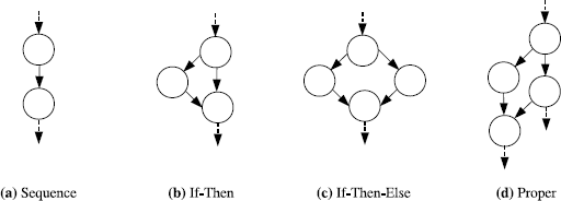
Sequential structural patterns
For the case of branches as shown in Figs. 15b and 15c, we compute safe overapproximations, since we take the maximum WCET of any path leading to the end block in line 6 of Algorithm 3. Similarly, we merge the result offsets of all paths reaching the end block in line 7 of the same algorithm. The last sequential case as shown in Fig. 15d is a combination of an if-then with a sequence. Therefore, the correctness for this case follows from the same arguments as in those cases.
-
Cyclic patterns
The possible cyclic patterns are shown in Fig. 16. We omitted patterns for loops which contain break or continue statements, since the generalization to these cases is a pure technicality. Theorems 4 and 5 from Sect. 5.2 show that our analysis framework correctly overapproximates the WCET and offset sets of loops (cyclic patterns). □
Fig. 16 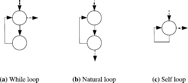
Cyclic structural patterns


In the proofs of correctness of the proposed “AnalyzeLoop” functions, we can use the induction hypothesis from Theorem 2, that \(\mathit{wcet}_{l}^{LB} ( O )\) and \(u_{l}^{LB} ( O )\) compute valid overapproximations.
Lemma 4
For two offset sets O 1 and O 2 with O 1⊆O 2 we observe that \(\mathit{wcet}_{l}^{LB} ( O_{1} ) \leq \mathit{wcet}_{l}^{LB} ( O_{2} )\) and \(u_{l}^{LB} ( O_{1} ) \subseteq u_{l}^{LB} ( O_{2} )\).
For \(\mathit{wcet}_{l}^{LB}\) this can be derived from the monotony of Φ p and for \(u_{l}^{LB}\) it can be derived from the monotony of the m and u b functions. Thus, \(\mathit{wcet}_{l}^{LB}\) and \(u_{l}^{LB}\) are monotone.
Theorem 3 For given starting offsets O in,l , the global convergence analysis computes safe overapproximations of the loop WCET and result offsets.
Proof
This proof handles the case of cyclic patterns in the proof of Theorem 2 and thus is a plug-in for this proof. If we would set \(O_{in}^{i} = O_{out}^{i-1}\) in the analysis, then we would perform a fully unrolling analysis, which would be unlikely to converge at any time step before the loop bound. The safeness of this fully unrolling analysis then follows from the safeness of the single-iteration analysis which we can assume since this is the induction hypothesis from Theorem 2. We use \(O_{in}^{i} = m ( O_{in}^{i-1}, O_{out}^{i-1} )\), therefore in our algorithm \(O_{in}^{i} \supseteq O_{out}^{i-1}\) holds. Lemma 4 implies that the WCET and offset results which we compute per iteration are overapproximations of the real WCET and offsets. This proves the correctness of the algorithm for the first j loop iterations. Then we have two cases:
-
\(j = B^{max}_{l}\)
In this case, all loop iterations were analyzed and thus the correctness of the analysis was shown for all loop iterations.
-
\(O_{in}^{j} = O_{in}^{j+1}\)
In this case, since \(O_{in}^{j}\) is a safe overapproximation of the offsets in loop iteration j and \(O_{in}^{j+1} = u_{l}^{LB} ( O_{in}^{j} )\) is a safe overapproximation of the offsets in loop iteration j+1, the loop can never be entered with offsets \(o \notin O_{in}^{j}\) in any succeeding iteration k>j. Therefore the offset and WCET results for the j-th iteration are safe overapproximations for all \(B^{max}_{l} - j\) remaining iterations. □
Lemma 2 For a loop l, assume O in,l is an overapproximation on the set of offsets at the entry of the loop before the first iteration. We claim that \(\mathit{reachable}(i) \supseteq O^{\mathrm{real}}_{i}\) is true for all iterations of the loop.
Proof
Let us assume that the construction of the offset graph terminates at iteration m (thus, m is the last iteration of the construction) and the loop bound is i. We prove the proposition by induction over the loop bound.
Base case: We can use the outer induction hypothesis, that the offset results computed by the single-iteration analysis are valid overapproximations. With O in,l being an overapproximation of the input offsets and i=1, this already proves the proposition since only a single loop iteration is modeled then.
Induction step: Due to the induction hypothesis we know that \(\mathit{reachable}(i) \supseteq O^{\mathrm{real}}_{i}\). We must show that \(\mathit{reachable}(i+1) \supseteq O^{\mathrm{real}}_{i+1}\) holds. To accomplish this, we assume that there is an offset \(o_{err} \in O^{\mathrm {real}}_{i+1}\) with o err ∉reachable(i+1). We will show that this leads to a contradiction.
If such an offset o err exists, then by definition of \(O^{\mathrm{real}}_{i+1}\) there must be a possible execution scenario A in which the (i+1)-th loop iteration is entered with offset o err . Let (a 1,a 2,…,a i+1) be the offsets with which the first i+1 iterations of the loop are entered in scenario A. Note that this implies a i+1=o err . Since we assume that o err ∉reachable(i+1), there must be at least two such offsets a p and a q for which \(( v_{a_{p}}, v_{a_{q}} ) \notin E\). Using the induction hypothesis it follows that a p ∈reachable(i) and thus that p=i and q=i+1.
Since a p is reachable in the graph, there must have been a construction iteration j<min(m,i) with \(a_{p} \in O_{out}^{j}\) and \(a_{p} \notin O_{in}^{j}\) where offset a p was reached for the first time. In construction iteration j+1 we add all edges \(E_{j+1} = O_{out}^{j} \times O_{out}^{j+1}\) to the graph. Since \(O_{out}^{j+1} = u_{l}^{LB} ( O_{out}^{j} )\) and \(a_{p} \in O_{out}^{j}\), it follows that \(a_{q} \in O_{out}^{j+1}\) since \(u_{l}^{LB}\) yields a safe overapproximation of the offsets and offset a p is followed by offset a q in scenario A. Therefore, we have \(( v_{a_{p}}, v_{a_{q}} ) \in E\) which is a contradiction. □
Theorem 4 Let us assume \(O^{real}_{in,l}\) is the set of offsets with which loop l may be entered in the first iteration. Given that \(O_{in,l} \supseteq O^{real}_{in,l}\), the graph tracking analysis always computes an overapproximation of the total execution time of the loop.
Proof
We prove this by induction on the loop bound \(B_{l}^{max}\).
Base case (\(B_{l}^{max}=1\): In this case, the objective function (Eq. (22)) simply takes the maximum of c(e) where e∈E transition and src(e)∈O in,l . Note that for any e∈E transition , c(e) represents the worst-case execution time of one loop iteration (computed by Algorithm 2) starting at offset src(e). Therefore, \(\max_{src(e) \in O_{in,l}} c(e)\) precisely represents the WCET of the first loop iteration. For \(B_{l}^{max}=1\) the ILP target function (Eq. (22)) is equal to this maximization, which proves the base case.
Induction step: We assume that the WCET computation is sound for loop bound \(B_{l}^{max} = n\). We shall show that the computation is also sound for loop bound \(B_{l}^{max}=n+1\). Let us assume that the actual WCET of the entire loop l with n iterations is denoted by WCET(l,n). On the other hand, the actual WCET of the n-th iteration of the loop is denoted by WCET iter (l,n). According to the graph tracking analysis, we compute the WCET of the loop with n+1 iterations as
where E is the set of all edges in the offset graph and T={0,…,n+1}. However,
where T′={0,…,n}. By induction hypothesis, we have
From Lemma 2 we know that \(\mathit{reachable}(n+1) \supseteq O^{\mathrm{real}}_{n+1}\). If an offset node is not reachable in iteration n+1, then it cannot contribute to Eq. (31), therefore
Inserting Eqs. (35) and (32) into Eq. (31) provides the induction step. Thus, the proposition is proven. □
Theorem 5 Computation of O out,l is sound. More precisely, O out,l predicted by the graph tracking analysis always overapproximates the set of offsets with which a loop may be left.
Proof
We are sending s l n c flow units through the graph. Each one of these units models an independent execution of the loop. Each of these modeled executions (say they are numbered with i∈{1,…,n c s l }) will exit the loop with some offset o end,i . The unknown set of all possible exit offsets is K. What we must show, is that K⊆{o end,i |i∈{1,…,n c s l }}.
What we maximize in Eq. (23) is the cardinality of the set of offsets with which the s l n c flow units exit the loop. By Lemma 2 the reachable offsets in the flow graph are an overapproximation of the reachable offsets in the real loop execution for all iterations \(j \in\{1,\ldots,B_{l}^{max}\}\). Therefore, if the loop can be left in iteration \(k \in\{B_{l}^{min}, \ldots, B_{l}^{max}\}\) with offset o left during a real loop execution, then it is possible to construct a flow with one flow unit i which starts at v + at time 0 and takes the edge \(e = (v_{o_{left}}, v^{-})\) at time step k, thus o end,i =o left for a given o left .
Up to this point we have then shown, that for each exit offset o left ∈K we can construct a flow with one flow unit that exits the loop with this offset. It is also possible that we get flows which end with offsets o err ∉K, but that is no problem since we only require an overapproximation of the offsets. If we now assume that we compute a solution O out,l with an offset k∈K and k∉O out,l , then we can easily show that this is a contradiction:
-
1.
|O out,l |=s l n c
In this case, the set O out,l represents all possible offsets, therefore an offset k∉O out,l cannot exist.
-
2.
|O out,l |<s l n c
In this case, there must be at least two flow units i and j with o end,i =o end,j , since we used F=n c s l flow units in total. Since k∈K holds, there exists a valid flow f through the graph which exits the loop with offset k (as shown in paragraph 2). If we let one of the flow units, say i, follow that flow f instead of the flow which it followed in the original solution, then we get a new solution to the flow problem in which |O out,l | is increased by 1, compared to the previous solution. Since the original solution to the flow problem must have been maximal with respect to |O out,l |, this is a contradiction. □
Corollary 1 The analysis framework, using the graph tracking analysis, provides overapproximations of the WCET of any task τ executed with starting offset O in,τ on our assumed platform.
Proof
Theorems 4 and 5 provide the missing induction step case for the proof of Theorem 2. The WCET for the \(f^{\mathrm{start}}_{\tau}\) function is the WCET of the task. Following Theorem 2, our analysis framework together with the graph tracking analysis produces valid WCET overapproximations for this function and thus also for the task. □
Rights and permissions
About this article
Cite this article
Kelter, T., Falk, H., Marwedel, P. et al. Static analysis of multi-core TDMA resource arbitration delays. Real-Time Syst 50, 185–229 (2014). https://doi.org/10.1007/s11241-013-9189-x
Published:
Issue Date:
DOI: https://doi.org/10.1007/s11241-013-9189-x