Understanding Kappa Distributions: A Toolbox for Space Science and Astrophysics

Abstract

In this paper we examine the physical foundations and theoretical development of the kappa distribution, which arises naturally from non-extensive Statistical Mechanics. The kappa distribution provides a straightforward replacement for the Maxwell distribution when dealing with systems in stationary states out of thermal equilibrium, commonly found in space and astrophysical plasmas. Prior studies have used a variety of inconsistent, and sometimes incorrect, formulations, which have led to significant confusion about these distributions. Therefore, in this study, we start from the N-particle phase space distribution and develop seven formulations for kappa distributions that range from the most general to several specialized versions that can be directly used with common types of space data. Collectively, these formulations and their guidelines provide a “toolbox” of useful and statistically well-grounded equations for future space physics analyses that seek to apply kappa distributions in data analysis, simulations, modeling, theory, and other work.

1 Introduction

Boltzmann-Gibbs (BG) Statistical Mechanics has withstood the test of time for describing classical systems in thermal equilibrium—a state where any flow of heat (e.g. thermal conduction, thermal radiation) is in balance. Any system in thermal equilibrium has its distribution function of velocities stabilized into a Maxwell distribution (in the absence of an external force). Maxwell distributions are quite rare in space and astrophysical plasmas (e.g. Hammond et al. 1996); instead, the vast majority of these plasmas reside in stationary states (i.e., their statistics are at least temporarily time invariant), that are typically not well described by Maxwell distributions, and thus not in thermal equilibrium.

Since Vasyliūnas (1968), empirical kappa distributions have successfully described plasmas in numerous locations, including: (1) the inner heliosphere, e.g., solar wind (e.g. Chotoo et al. 2000; Mann et al. 2002; Zouganelis et al. 2004; Maksimovic et al. 2005; Marsch 2006; Yoon et al. 2006; Pierrard and Lazar 2010), and planetary magnetospheres (e.g. Christon 1987; Collier and Hamilton 1995; Mauk et al. 2004; Schippers et al. 2008; Dialynas et al. 2009; Ogasawara et al. 2012), (2) the outer heliosphere and the inner heliosheath (e.g. Decker and Krimigis 2003; Decker et al. 2005; Heerikhuisen et al. 2008, 2010; Zank et al. 2010; Livadiotis et al. 2011, 2012, 2013; Livadiotis and McComas 2012a), and (3) other various plasma-related analyses (e.g. Milovanov and Zelenyi 2000; Saito et al. 2000; Leubner 2004; Raadu and Shafiq 2007; Baluku et al. 2010; Livadiotis and McComas 2009, 2010a, 2011b; Le Roux et al. 2010; Eslami et al. 2011; Kourakis et al. 2012; see also the work of Tribeche and collaborators in dusty plasmas, e.g., Tribeche et al. 2009, 2012; Tribeche and Bacha 2010; Tribeche and Merriche 2011; Roy et al. 2012; Bains et al. 2013). Because BG Statistical Mechanics cannot adequately describe non-equilibrium plasmas, new advances were required. Fortunately, recent developments have shown that the generalized framework of non-extensive Statistical Mechanics, offers a solid theoretical basis for describing such systems in non-equilibrium stationary states (e.g. Tsallis 1988, 2009, 2011; Tsallis et al. 1998; Borges et al. 2002; Livadiotis and McComas 2009).

The statistical behavior of space plasmas is related to their nature as collisionless and weakly coupled plasmas, with large numbers of particles in a Debye sphere. Weakly coupled plasmas are not governed by interactions between individual particles, but instead the overall collective electrostatic forces of many particles. Strong interactions between individual particles are relatively rare and cause little if any sudden change in the particles’ motion, which is largely governed by its kinetic energy. Therefore, space plasmas show strong collective behavior that characterizes the correlated particles within a Debye sphere, without localized phenomena between individual particles due to interactions or collisions. This behavior leads these systems to exotic statistical states that cannot be understood by the classical statistical description of thermal equilibrium.

While several analyses successfully extract the kappa distribution from basic physical mechanisms and processes related to the nature of space plasmas (e.g. velocity-space diffusion, Hasegawa et al. 1985; kinetic theory with correlations, Treumann 1999; Langmuir turbulence, Yoon 2012), the most direct approach is to derive these distributions within a physically meaningful statistical framework. Kappa distributions naturally emerge from the first principles and basic paths in non-extensive Statistical Mechanics (see Appendix A and Tsallis 2009); the connection between non-extensive Statistical Mechanics and kappa distributions was developed in detail by Livadiotis and McComas (2009; see also 2010a, 2010b, 2010c, 2011b).

Since the observational formulation of Vasyliūnas (1968), kappa distributions have become one of the most widely used tools for characterizing and describing space plasma populations (Fig. 1). Now that the underlying statistical physics basis for these distributions has been shown, it is more important than ever to develop and investigate the basic formulations for kappa distributions.

Fig. 1

(a) Number and (b) cumulative distribution of N∼1600 papers cataloged in Google Scholar from 1980 through 2012 that are related to kappa distributions and include these distributions in their title. The fit curve (blue dash) in both panels show the exponential growth of these studies

In Sect. 2 we review the basic characteristics of the statistical mechanics and thermodynamics of non-equilibrium systems such as space plasmas. In Sect. 3 we develop seven kappa distribution formulations, which comprise the basic toolbox for describing the statistics of systems out of thermal equilibrium; these range from the most general to several specialized versions that can be directly used with common types of space data. Section 4 briefly summarizes and discusses the conclusions. Two appendices support the article: Appendix A provides the fundamental principles and properties of non-extensive Statistical Mechanics, and Appendix B develop and prove the mathematical formulations provided in the toolbox.

2 Statistical Mechanics and Thermodynamics of Space Plasmas

Non-extensive Statistical Mechanics is a self-consistent generalization of the classical formalism of Boltzmann-Gibbs Statistical Mechanics and can describe many systems where classical statistical physics fails. In particular, it can describe systems with continuous energy spectra that are out of thermal equilibrium. The basic principle is the generalized entropy formulation, which fulfills all the required conditions of a physically meaningful entropic function (Tsallis 2009): (i) Non-negativity, (ii) maximization at equidistribution, (iii) Non-additivity, (iv) Experimental Robustness, (v) Uniqueness. For details on the basic principles and characteristics of non-extensive Statistical Mechanics, see Appendix A.

The Maxwell distribution of velocities can be derived following the Gibbs path by maximizing the BG entropy under the constraints of the Canonical Ensemble. Similarly, the kappa distribution of velocities can be obtained by maximizing the generalized entropy of non-extensive Statistical Mechanics; this is called Tsallis entropy, and is parameterized by the q-index (Tsallis 1988). While the Maxwell distribution is the Canonical distribution in the classical framework of BG Statistical Mechanics that applies only at thermal equilibrium, the kappa distribution is the Canonical distribution in the generalized framework of non-extensive Statistical Mechanics that applies both in and out of thermal equilibrium. In fact, the kappa distribution reverts to a Maxwell distribution for κ→∞. In the Statistical Physics community the kappa distribution is better known as q-exponential or q-Maxwellian distribution. Livadiotis and McComas (2009) showed the absolute equivalence of the q-exponential distribution and the kappa distribution, demonstrating the connection required for the statistical grounding of the kappa distribution, and provided the fundamental relationship between the entropy’s q-index and the distributions’ κ-index: q=1+1/κ.

The greatest challenge for the foundation of Statistical Mechanics and Thermodynamics for non-equilibrium systems described by kappa distributions was to assign an actual physical meaning to temperature out of thermal equilibrium. For nearly half a century, space plasma “temperatures” have been calculated from the second statistical moment of their velocity distributions. While this method is correct for distributions in thermal equilibrium, there was no a priori reason to believe that this was a well-defined temperature out of equilibrium. For example, what is the outcome of mixing two non-equilibrium plasmas (possibly via magnetic reconnection)? Is it similar to the mixing of classical gases, which obey simple calorimetry rules (e.g. if we mix two plasmas with different temperatures and densities, will that result in a mass-weighted average temperature of the combined plasma)? This quandary was recently resolved by demonstrating the equivalence of the two basic temperature definitions, (1) kinetic and (2) thermodynamic, for kappa distributions of particles out of equilibrium (Livadiotis and McComas 2009, 2010a).

The mean kinetic energy provides the kinetic definition of temperature (Maxwell 1866), $\langle \mathrm{K} \rangle= \langle\frac{1}{2}m(\boldsymbol{u} - \boldsymbol{u}_{b})^{2} \rangle= \frac{3}{2}k_{\mathrm{B}}T$. Equivalently, this is expressed by the variance of the velocity distribution, $\langle(\boldsymbol{u} - \boldsymbol{u}_{b})^{2} \rangle= \frac{3}{2}\theta ^{2}$. (θ is the temperature expressed in speed units; note that all symbols used in this paper are defined in Table 1.) Since the mean kinetic energy defines (kinetically) the temperature, it cannot be depended on any parameter (such as the kappa index) except the actual temperature. This realization forced the rejection of several previous approaches, where the mean kinetic energy depended on both the kappa index and some other thermal parameter that tried to provide an interpretation of temperature (Livadiotis and McComas 2009). It is also important to note that the kinetic definition of temperature is given only by the second statistical moment of the velocities and not by any other statistical moment. For example, the ath statistical moment, μ _a ≡〈|u−u _b |^a〉, a>0, cannot define the temperature, because it depends also on κ (for any a≠2).

Table 1 Involved variables, functions, and parameters

In contrast to the kinetic definition, the thermodynamic definition of temperature is given by the connection of entropy S with the internal energy U (in the absence of a potential energy, it is given by the mean kinetic energy, U=〈K〉) (Clausius 1862), $T \equiv(\partial S/\partial U)^{ - 1} \cdot[1 - \frac{1}{\kappa} \cdot S/k_{\mathrm{B}}]$. Note that only this type of connection is consistent with the zero-th law of Thermodynamics (Abe 2001). Livadiotis and McComas (2009) showed the equality between these two different temperature definitions—the kinetic and thermodynamic, and thus produced a well-defined temperature for systems out of thermal equilibrium that are describable by kappa distributions (see also Livadiotis and McComas 2010a). These innovations allowed a generalization of zero-th law of Thermodynamics, “Two bodies that are in equilibrium with a third are in equilibrium with each other”, to cover stationary states out of equilibrium: “Two bodies that are in equilibrium or the same non-equilibrium stationary state with a third, are in the same stationary state with each other” (Livadiotis and McComas 2010a).

Once the physical meaning of temperature was established for systems out of thermal equilibrium, other relevant thermodynamic parameters could be also defined. For example, the thermal pressure P=nk _B T and the polytropic index ∂logn/∂logT were examined for non-equilibrium systems by Livadiotis and McComas (2012a). Moreover, because of its independence from the other parameters, the kappa index can now be understood as a unique thermodynamic variable just like temperature and density, but in contrast to these, kappa characterizes the non-equilibrium systems and their transitions through different stationary states.

The possible values of the kappa index are $\kappa\in(\frac {3}{2},\infty]$ (for more details, see Livadiotis and McComas 2010a). For κ→∞, the system resides at thermal equilibrium, while for $\kappa\to\frac{3}{2}$, the system approaches the furthest state from equilibrium, or “anti-equilibrium”; Livadiotis and McComas (2010a) used the term “q-frozen state” from non-equilibrium statistical mechanics, however here we are proposing the new name—anti-equilibrium in order to encapsulate the much broader range of properties of this unique state.

The extreme stationary states, equilibrium and anti-equilibrium, have characteristic universal behavior that are independent of the system’s dimensionality f. At equilibrium (κ→∞), the kappa distribution reverts to the Maxwellian distribution of velocities ∼exp{−(u−u _b )²/θ ²}. At anti-equilibrium (κ→3/2), the kappa distribution approaches a power-law distribution that naturally produces the “ubiquitously observed” flux-energy power-law ∼ε ^−1.5 (e.g. Fisk and Gloeckler 2006). This statistical behavior is independent of the values of the other thermodynamic parameters or of the system’s dimensionality. Having this universal behavior of the two extremes, it is meaningful to determine the “thermodynamic distance” of a given state from thermal equilibrium (Fig. 2). A measure of this “thermodynamic distance” can be defined by fulfilling certain mathematical conditions (Livadiotis and McComas 2010b, 2010c).

Fig. 2

The complete spectrum of all possible kappa indices, or “kappa spectrum”. The whole set of stationary states exists in a spectrum-like arrangement of the κ-index over the interval 3/2<κ≤∞. The indices κ→∞ and κ→3/2 correspond to thermal equilibrium and the furthest possible state from equilibrium (anti-equilibrium), respectively. Both the extreme states have universal behavior: At κ→∞, the distribution is reduced to the Maxwellian exponential, while at κ→3/2, the flux-energy spectra are described by the power-law ∼ε ^−1.5. This universality suggests that the maximum “thermodynamic distance” between the extreme states (equilibrium and anti-equilibrium) is fixed, and thus, the furthest state can be referred to as 100 % away from equilibrium, while all the stationary states can be arranged according to the thermodynamic distance lying between the extreme states of equilibrium (0 %) and anti-equilibrium (100 %)

The physical meaning of the kappa index is interwoven with the correlation of particles in systems out of thermal equilibrium. One of the crucial limitations of the classical BG Statistical approach is that correlations between particles are not included. By contrast, the non-extensitivity of Statistical Mechanics naturally captures the correlations between the particles and the degrees of freedom. In particular, the correlation is mathematically modeled by the specific formulation of the kappa distribution, that cannot be factored. If P(ε ₁,ε ₂) is the joint probability distribution, and P(ε ₁), P(ε ₂) are the individual marginal probability distributions of two particles with energies ε ₁ and ε ₂, then, the factorization of the joint distribution is P(ε ₁,ε ₂)=P(ε ₁)⋅P(ε ₂). For example, the exponential distribution can always be factored. This mathematical property is equivalent to the absence of correlation in systems described by the Maxwell distribution. On the other hand, the kappa distribution cannot be factored, P(ε ₁,ε ₂)≠P(ε ₁)⋅P(ε ₂), and there is a non-zero correlation coefficient ρ between the energies of any two particles of a system. Livadiotis and McComas (2011b) showed that $\rho= \frac{3}{2}/\kappa$, producing the “kappa spectrum” shown in Fig. 2. Therefore, the classical case of systems residing in thermal equilibrium (κ→∞) assumes no correlation (ρ→0), while the other extreme state of “anti-equilibrium” ($\kappa \to\frac{3}{2}$) indicates a maximum correlation (ρ→1).

Both the basic independent thermodynamic parameters, T and κ, can be expressed in terms of the individual kinetic energies of the particles, that is through their mean value and correlation, respectively. It is important to note that only the kinetic part of the energies can be involved in the expressions of T and κ. If both the kinetic and potential energy were involved, i.e., by deriving the mean value or correlation of the total energy, the resulting pseudo-“temperature” and “kappa” would be incorrect and not physically meaningful.

Finally we note that the fundamental physical meaning of correlation is tied into the organization of plasmas by their Debye shielding within clusters of locally correlated particles (Debye spheres). Livadiotis and McComas (2013c) recently began developing this concept for non-equilibrium space plasmas, and showed that a Debye sphere of correlated particles is characterized by a minimum energy exchange and lifetime, leading to a large-scale phase-space quantization, 12 orders of magnitude larger than the Planck constant.

The kappa index is of great importance for understanding, classifying, and studying the non-equilibrium stationary states. However, the kappa index must be invariant of the system’s size, namely, independent of the system’s kinetic degrees of freedom f that include the number of particles N and kinetic degrees of freedom per particle d i.e., f=N⋅d. Livadiotis and McComas (2011b) showed that the widely used kappa index κ, is actually dependent on f, and can be related to an invariant and fundamental kappa index κ ₀ by $\kappa(f) = \kappa _{0} + \frac{1}{2}f$. Given the large number of particles N, it appears that the value of the dependent kappa index should be huge; however, the actual kappa index that characterizes a stationary state is κ ₀, which is invariant from the number of particles and degrees of freedom of the system. Indeed, the system is still described by a kappa distribution, even when κ(f)→∞ (as shown in Eq. (B.2) of Appendix B). The usage of the invariant kappa index allowed, for the first time, the development of invariant formulations of kappa distribution functions of velocity and energy, and showed that these formulations encompass the entire N-particle phase space distribution (Livadiotis and McComas 2011b; see also Appendix B). The N-particle distribution is the joint probability distribution of the phase space, P(r ₁,u ₁,r ₂,u ₂,…,r _N ,u _N ), or of the energies, P(ε ₁,ε ₂,…,ε _N ), of all the N particles of a system. The 1-particle distribution of phase space, P(r,u), or energy, P(ε), comes from integrating over N−1 particles’ phase spaces or energies; it constitutes the simplest way to study the phase-space distribution of particles and is a good approximation when the system’s particles are weakly interacting and nearly uncorrelated. This is true for systems residing at thermal equilibrium, but for non-equilibrium systems, a great deal of information is lost when reducing an N-particle to a 1-particle description. Throughout the paper, we may refer to the invariant kappa index, using the notions of κ ₀ or $\kappa= \kappa_{0} + \frac{3}{2}$.

As a system approaches absolute zero (for a fixed kappa index), the distribution maximum shifts to smaller velocities/energies, thus producing a phenomenological deceleration of the particles toward freezing. Such a phenomenological deceleration of particles can also be realized by decreasing the kappa index. Therefore, variations in the kappa index can act in a temperature-like fashion (Livadiotis and McComas 2010a, 2011b). While the mean energy or temperature is independent of the kappa index, it turns out that decreasing the kappa index produces a different kind of “freezing”, where particles decelerate to near zero velocities/energies, being absolutely frozen (if we ignore quantum fluctuations) at the limit of anti-equilibrium ($\kappa\to \frac{3}{2}$). Close to the anti-equilibrium limit, the mode of the distribution is compressed near the zero energy, while all the non-zero energies become very unlikely. This peculiar behavior of the kappa index imitating the temperature at extremely far from equilibrium states suggests the combining of two parameters, the temperature k _B T (in energy units) and the invariant kappa index κ ₀ of a system, into a single product, Θ≡κ ₀⋅k _B T, that encapsulates both. Livadiotis and McComas (2010a) showed that the limit of the kappa distribution could then be expressed in terms of Θ alone, since the two independent thermodynamic variables, κ, T degenerate into a single variable at anti-equilibrium.

Space plasma observations have shown an empirical separation of the κ-spectrum. This spectrum (Fig. 2) is divided into near- and far-equilibrium regions with a separatrix at κ∼2.5: indices 2.5<κ≤∞ (e.g. Saturnian magnetosphere, Dialynas et al. 2009) represent near-equilibrium, while the far-equilibrium region has indices 1.5<κ≤2.5 (e.g. inner heliosheath, Livadiotis et al. 2011). Indeed, various space plasmas appear to have indices distributed essentially over only one or the other region. For example, solar wind is characterized by κ-indices in the near-equilibrium region (e.g., Livadiotis and McComas 2013a), while heavy ions during quiet times (Dayeh et al. 2009), interplanetary shocks (Desai et al. 2004), and corotating interaction regions (Mason et al. 2008) are characterized by κ-indices in the far-equilibrium region.

One intriguing case of far- and near-equilibrium plasmas comes from comparing the inner heliosphere and the inner heliosheath proton plasmas. Indeed, the inner heliosphere is typically characterized by kappa indices in the near-equilibrium region (Livadiotis and McComas 2012b), while the kappa indices in the inner heliosheath were found to be restricted to the far-equilibrium region (Livadiotis et al. 2011), as measured via Energetic Neutral Atoms (ENAs) from the Interstellar Boundary EXplorer (IBEX) (McComas et al. 2009a, 2009b). This may be surprising because the inner heliosheath is largely populated by solar wind plasma that has traveled out beyond the termination shock, and because both the additional time for it to evolve and the action of shock heating might be expected to push the plasma closer to equilibrium. However, Livadiotis and McComas (2010a) anticipated this dissimilar behavior of kappa indices between the inner heliosphere and inner heliosheath, by proposing that pick-up protons, which are ions with highly organized phase-space distributions, can reduce the entropy of the combined system of solar wind and pick-up protons, and thus push the values of the kappa index toward the far-equilibrium region. This result was first shown based on analytical work (Livadiotis and McComas 2011a), and then verified by analyzing IBEX ENA observations (Livadiotis et al. 2011). In theory, there is no reason that by adding a pick-up proton distribution to a solar wind kappa distribution, their sum will end up again as some kappa distribution. On the other hand, remote ENA observations from IBEX indicate that the inner heliosheath does appear to have one proton population, that includes the incorporated pick-up and solar wind protons, and this follows a distribution that matches a kappa distribution (Livadiotis et al. 2013). Hence, the entropy of the system can inform us about the final kappa index (Livadiotis and McComas 2011a).

The thermodynamics of the far-equilibrium region are much more complicated than that of the near-equilibrium region. This is shown by the entropy when expressed only in terms of the kappa index; this is monotonic for 2.5<κ≤∞ and non-monotonic convex with a minimum for 1.5<κ≤2.5 (Fig. 3). (For more details, see: Livadiotis and McComas 2010a, 2010c, 2013b.)

Fig. 3

(a) Spontaneous increases of entropy move the system gradually toward thermal equilibrium, within the near-equilibrium region, κ>2.5. On the other hand, external factors that may decrease entropy, move the system back away from equilibrium, into the far-equilibrium region, κ≤2.5. Newly formed pick-up ions can play this critical role in the case of solar wind and other space plasmas, because of their highly ordered motion. They reduce the entropy of the system and move it toward the far-equilibrium region. (b) Distribution of κ-indices D(κ) for the inner heliosheath protons H⁺

The basic thermodynamic processes, such as isothermal (constant temperature T), isochoric (constant number density n), isobaric (constant pressure P), characterize systems at thermal equilibrium. These three parameters are related to the other two through the equation of state P=nk _B T, so the three really only represent two independent variables. For systems out of thermal equilibrium such as the majority of space plasmas, the phase space is characterized also by a third independent parameter, the κ-index. Typically, in space plasmas (T,n) are considered as the two independent parameters (where the pressure is dependent).

Moreover, systems may attribute specific polytropic laws that correlate the two parameters. A single-polytrope means that for some systems T and n are simply related by n∼T ^ν, or, ν=∂logn/∂logT, while a multi-polytrope means the general relation of a variable polytropic index, ν(T). Hence, the general polytrope can be expressed by f(T,n)=0 when κ is fixed (e.g. at thermal equilibrium where the kappa index is fixed to κ→∞), and f(T,n;κ)=0 for a variable κ. The thermodynamic processes for non-equilibrium systems can be arranged according to the relation between {T,n,P} and κ, as shown in Table 2.

Table 2 Non-equilibrium thermodynamic processes

As an example of non-equilibrium thermodynamic processes, Fig. 4 plots the kappa indices and temperature of the inner heliosheath observed by IBEX, as derived from Livadiotis et al. (2011). Using the IBEX-Hi energy-flux ENA spectra, these authors constructed the sky maps of the (radially) average temperature and density (among other thermal observables) of the ENA-source proton populations in the inner heliosheath. This was enabled by connecting the observed ENA flux to the parametric distribution of velocities of the source protons (as was also shown in Livadiotis et al. 2012, 2013). While theoretically, the entire (T, n, κ) space could be filled, these authors found that the inner heliosheath distributions followed only narrow curves in this space. Figure 4 shows the coupling between the parameters of the inner heliosheath, where we observe the thermodynamic processes: (1) isobaric (dominant over the vast majority of the sky map pixels), (2) roughly isothermal with state transitions at low latitudes near the equator, (3) stationary state at higher latitudes near the poles. (Livadiotis and McComas 2012a, 2013a; Livadiotis et al. 2013.)

Fig. 4

Thermodynamic diagrams of proton plasma in the inner heliosheath: (a) κ–logT, indicating isothermal and single stationary state processes, (b) logn–logT, with slope 1/ν∼−1 indicating isobaric processes. The color coding separates the enhanced ENA fluxes of the IBEX Ribbon (red) from the globally distributed ENA flux (McComas et al. 2009b; Schwadron et al. 2011), that has been further divided into regions near the equator (green) and near the poles (blue) (Livadiotis et al. 2011)

3 Using Kappa Distributions: The Toolbox

Here we develop the seven kappa distribution formulations, which are the basic tools for describing the statistics of systems out of thermal equilibrium (see Appendix A for analytical derivations). We briefly provide consistent and useful information for each of these tools, including: nomenclature, properties, formulae, description, usage, and some examples of applications. These seven basic formulations are connected together via a derivation scheme, as shown in Fig. 5. Real-world, N-particle distributions can be reduced to 1-particle distributions, which are more convenient to handle but less accurate, for describing the statistics of a system. Similarly, the distributions of Hamiltonian are more general, but they can be reduced to distributions of velocities for cases when potential energy can be ignored.

Fig. 5

The Kappa distribution toolbox and the connections between the seven basic formulations. Abbreviation mnemonics are given in square brackets based on the variable symbols of the involved equations (i.e., $\vec{\mathrm{U}}$: velocity, U: speed, E: energy, Ω: angles). The left and right columns include the N-particle (red) and 1-particle (blue) representations, respectively. The first and second rows include the Hamiltonian and kinetic energy distributions, respectively. While the first two rows pertain to velocity vectors, the last two rows (green) include the velocity magnitude (speed) or energy, and/or angular direction

For the seven tools described below, we use the variables, functions, and parameters included in Table 1.

3.1 N-Particle Kappa Distribution of Hamiltonian

• 1. Tool Symbol: [NH].

• 2. Properties: N-particle, (2d⋅N)-dimensional distribution; it applies to the (2d⋅N)-dimensional phase space.

• 3. Formulation:

  

  (3.1)
  

  (3.2)

  with the potential normalization constant being equal to

  $$ {A}_{\varPhi} (\kappa_{0},T;N) \equiv\biggl\{ \int _{\boldsymbol{r}_{n} \in V} \biggl[ 1 + \frac{1}{\kappa_{0}} \cdot\frac {1}{k_{\mathrm{B}}T} \cdot\varPhi\bigl(\{ \boldsymbol{r}_{n}\} \bigr) \biggr]^{ - \kappa_{0} - 1}d\boldsymbol{r}_{1}d\boldsymbol{r}_{2} \cdots d\boldsymbol{r}_{N} \biggr\}^{ - 1}. $$

  (3.3)

• 4. Description:

  • Describes the phase space distribution of all the particles of a system.

  • The Hamiltonian is given by $H(\{ \boldsymbol{r}_{n}\},\{ \boldsymbol{w}_{n}\} ) = H(\{ \boldsymbol{r}_{n}\},\{ \boldsymbol{u}_{n}\};\boldsymbol{u}_{b}) = \frac{1}{2}m\sum_{n = 1}^{N} (\boldsymbol{u}_{n} - \boldsymbol{u}_{b})^{2} + \varPhi(\{ \boldsymbol{r}_{n}\} )$.

  • The position vectors {r _n } span the system’s volume V.

  • In space physics the velocities are typically used to describe the phase space, instead of the standard use of momentums {m u _n }.

  • Non-extensive Statistical Mechanics requires that the Hamiltonian function is included such that the internal energy, i.e., the average Hamiltonian 〈H〉, is normalized to zero in the canonical distribution, i.e., H({r _n },{w _n })→H({r _n },{w _n })−〈H〉. Thus, the potential energy is appropriately constructed so that 〈Φ〉=0, otherwise, Φ({r _n }) must be replaced by Φ({r _n })−〈Φ〉 in the whole analysis.

  • In the above formulation, the potential energy is considered non-negative, Φ≥0. However, in the case it is negative, Φ<0, the quantity 1+H/(κ ₀ k _B T) may also be negative. In this case, the distribution is zero owing to the Tsallis cut-off condition (Tsallis 2009). Hence, the distribution is meaningful when 1+H/(κ ₀ k _B T)≥0, which gives K≥|Φ|−κ ₀ k _B T. We note the following: (i) The inequality adds no new information for κ ₀→∞ (thermal equilibrium), while it is important away from equilibrium, e.g. for κ ₀→0 (near anti-equilibrium), i.e., K≥|Φ|. (ii) The inequality affects the normalization of the distribution, for which the velocities must be integrated starting from their relevant lower limit that corresponds to the smaller kinetic energy limit |Φ|−κ ₀ k _B T., i.e., |Φ|−κ ₀ k _B T≤K<∞. (iii) Space plasmas are typically weakly coupled and any internal or external potential energy is usually substantially smaller than the kinetic energy (see Introduction). Therefore, the contribution of the portion 0≤K≤|Φ|−κ ₀ k _B T may generally be ignored, and the normalization can be estimated by integrating over 0≤K<∞. (For an example with negative potential, see: Tribeche and Bacha 2010.)

  • The normalization provided does not include more complicated cases where the potential energy depends also on the velocities; such normalizations can be derived, based on the detailed formulation of the specific potential energy for that system.

• 5. Usage:

  • Models the phase space distribution of all the particles of a system when the potential energy is not small compared to the kinetic energy, thus cannot be ignored.

  • Achieves accurate plasma simulations.

  • Derives the expectation value of any function of the positions or the velocities, f({r _n },{u _n }), i.e., 〈f〉=∫f({r _n },{u _n })⋅P({r _n },{u _n })d r ₁ d r ₂⋯d r _N d u ₁ d u ₂⋯d u _N .

• 6. Applications: The Hamiltonian that describes the phase space of all the particles of a system in a weak external gravitational field is $H(\{ z_{n}\},\{ \boldsymbol{u}_{n}\};\boldsymbol{u}_{b}) = \frac{1}{2}m\sum_{n = 1}^{N} (\boldsymbol{u}_{n} - \boldsymbol{u}_{b})^{2} + \varPhi(\{ z_{n}\} )$, where Φ approximates the gravitational potential energy $\varPhi(\{ z_{n}\} ) = mg \cdot\sum_{n = 1}^{N} z_{n}; z _{n}$ measures the height of the nth particle; g is the gravitational acceleration. The potential energy’s zero level is 〈z〉=0, corresponding to 〈Φ〉=0.

3.2 N-Particle Kappa Distribution of Velocities

• 1. Tool Symbol: [$\mathrm{N}\vec{\mathrm{U}}$].

• 2. Properties: N-particle, (d⋅N)-dimensional distribution; it applies to the (d⋅N)-dimensional velocity space.

• 3. Formulation:

  

  (3.4)

• 4. Description:

  • Describes the distribution of all the particle velocities of a system.

  • It applies when the potential energy is small and ignored compared to the kinetic energy.

  • It describes the statistics of particles more accurately than the one-particle distribution.

• 5. Usage:

  • Models the distribution of all the particle velocities of a system.

  • Achieves accurate plasma simulations.

  • Derives thermodynamic parameters (e.g. entropy), or the expectation value of any function of the velocities, f({u _n }), i.e., 〈f〉=∫f({u _n })⋅P({u _n })d{u _n }.

• 6. Applications: The entropy is the expectation value of the function f({u _n })=I[P({u _n })], where the functional I(P) is called “information measure” (Gell-Mann and Tsallis 2004). (For details see Livadiotis and McComas 2013b.)

3.3 1-Particle Kappa Distribution of Hamiltonian

• 1. Tool Symbol: [1H].

• 2. Properties: 1-particle, 2d-dimensional distribution; it applies to the 2d-dimensional phase space.

• 3. Formulation:

  

  (3.5)
  

  (3.6)

  with the potential normalization constant being equal to

  $$ {A}_{\varPhi} (\kappa_{0},T) \equiv\biggl\{ \int _{\boldsymbol{r} \in V} \biggl[ 1 + \frac{1}{\kappa_{0}} \cdot\frac{1}{k_{\mathrm{B}}T} \cdot\varPhi(\boldsymbol{r}) \biggr]^{ - \kappa_{0} - 1}d\boldsymbol{r} \biggr\}^{ - 1}. $$

  (3.7)

• 4. Description:

  • Describes the phase space distribution of a particle.

  • The Hamiltonian is given by $H(\boldsymbol{r},\boldsymbol{\boldsymbol{u}};\boldsymbol{\boldsymbol{u}}_{b}) = \frac{1}{2}m(\boldsymbol{\boldsymbol{u}} - \boldsymbol{\boldsymbol{u}}_{b})^{2} + \varPhi(\boldsymbol{r})$.

  • The position vector r spans the system’s volume V.

  • The potential energy is appropriately constructed so that 〈Φ〉=0, otherwise, Φ(r) must be replaced by Φ(r)−〈Φ〉 in the whole analysis.

• 5. Usage:

  • Models the phase space distribution of a particle of a system, when the potential energy is not small compared to the kinetic energy, thus cannot be ignored.

  • Simulations or theoretical derivations may deviate from the more accurate results of using the N-particle kappa distribution.

  • Estimates the expectation value of any function of the positions or the velocities of a particle, f(r,u), i.e., 〈f〉=∫f(r,u)⋅P(r,u)d r d u.

• 6. Applications: The gravitational Hamiltonian for the 1-particle phase space description is given by $H(z,\boldsymbol{\boldsymbol{u}};\boldsymbol{\boldsymbol{u}}_{b}) = \frac{1}{2}m(\boldsymbol{\boldsymbol{u}} - \boldsymbol{\boldsymbol{u}}_{b})^{2} + \varPhi(z)$, where Φ approximates the weak gravitational potential energy Φ(z)=mg⋅z. The potential energy’s zero level corresponds to 〈z〉=0, so that 〈Φ〉=0.

3.4 1-Particle Kappa Distribution of Velocities

• 1. Tool Symbol: [$1\vec{\mathrm{U}}$].

• 2. Properties: 1-particle, d-dimensional distribution; it applies to the d-dimensional space of velocities.

• 3. Formulation:

  

  (3.8)

  The distribution is isotropic in the co-moving frame with velocity w≡u−u _b and energy $E = \frac{1}{2}m(\boldsymbol{u} - \boldsymbol{u}_{b})^{2}$,

  • Speed:

    $$ P_{\mathrm{V}}(w;\kappa_{0},\theta) = \frac{2\kappa_{0}^{ - \frac {d}{2}}}{{B}(\kappa_{0} + 1,\frac{d}{2})} \cdot \theta^{ - d} \cdot\biggl( 1 + \frac{1}{\kappa_{0}} \cdot \frac{w^{2}}{\theta^{2}} \biggr)^{ - \kappa_{0} - 1 - \frac {d}{2}}w^{d - 1}. $$

    (3.9)

  • Energy:

    

    (3.10)

    where B(x,y)≡Γ(x)Γ(y)/Γ(x+y) is the Beta function; $F(x;m,n)=B(\frac{m}{2},\frac{n}{2})^{-1} \cdot x^{n/2-1} \cdot (1+x)^{-(m+n)/2}$ is the F-distribution (Abramowitz and Stegun 1972).

  • For d=3:

    

    (3.11)

  • For $\kappa= \kappa_{0} + \frac{3}{2}$:

    

    (3.12)

  Special cases:

  • (i) Behavior at equilibrium and anti-equilibrium:

    • κ→∞:

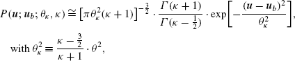
      $$ P(\boldsymbol{u};\boldsymbol{u}_{b};\theta) = \pi^{ - \frac{3}{2}}\theta^{ - 3} \cdot \exp\biggl[ - \frac{(\boldsymbol{u} - \boldsymbol{u}_{b})^{2}}{\theta^{2}} \biggr], $$

      (3.13)

      that is normalized for 0≤|u−u _b |<∞,

    • $\kappa\to\frac{3}{2}$:

      $$ P(\boldsymbol{u};\boldsymbol{u}_{b};\theta;\kappa) = \frac{1}{3\pi} \biggl(\kappa- \frac{3}{2}\biggr)\theta^{2} \cdot \vert \boldsymbol{u} - \boldsymbol{u}_{b} \vert ^{ - 5}, $$

      (3.14)

      that is normalized for |u−u _b |_Max≤|u−u _b |<∞, $\vert \boldsymbol{u} - \boldsymbol{u}_{b} \vert _{\mathrm{Max}} = \theta\cdot \sqrt{(\kappa- \frac{3}{2})/\kappa}$.

  • (ii) Approximations near the core (small speeds/energies) and tail (large speeds/energies):

    • Core, $(\boldsymbol{u} - \boldsymbol{u}_{b})^{2} \ll (\kappa- \frac{3}{2})\theta^{2}$:

      

      (3.15)

    • Tail, $\boldsymbol{u}^{2} \gg (\kappa- \frac{3}{2})\theta^{2}$, $\boldsymbol{u}^{2} \gg \boldsymbol{u}_{b}^{2}$:

      $$ P(\boldsymbol{u};\theta,\kappa) \cong \pi^{\frac{3}{2}} \frac{\varGamma(\kappa+ 1)}{\varGamma(\kappa- \frac{1}{2})} \biggl[\biggl(\kappa- \frac{3}{2}\biggr)\theta^{2}\biggr]^{\kappa- \frac{1}{2}} \cdot \vert \boldsymbol{u} \vert ^{ - 2\kappa- 2}. $$

      (3.16)

      (The approximations lead to unnormalized distributions.)

• 4. Description:

  • Describes the velocity distribution of a single particle.

  • The potential energy is ignored.

• 5. Usage:

  • Provides the easiest way to model the velocity distribution of a particle of a system.

  • Simulations or theoretical derivations may deviate when using the more accurate N-particle kappa distribution.

  • Estimates the expectation value of any function of the velocities of a particle, f(u), i.e., 〈f〉=∫f(u)⋅P(u)d u, e.g. the ath statistical moment is the expectation value of the function f(u)=|u−u _b |^a.

• 6. Applications: Ion/electron velocities recorded by Ulysses/SWOOPS (Bame et al. 1992) are given in 3-dimensional vectors u. For a given time integral Δt, the bulk velocity u _b is estimated as the mean velocity of the included measurements. Then, the distribution of |u−u _b | is constructed and compared with P(u;u _b ;θ,κ ₀) (for d=3) (e.g. see an example in Livadiotis and McComas 2013a).

3.5 Kappa Distribution of Speed/Energy at an Angular Direction

• 1. Tool Symbol: [UEΩ].

• 2. Properties: 1-particle, 1-dimensional distribution; independent variables: speed (velocity magnitude) or energy.

• 3. Formulation:

  • Speed:

    $$ P_{\mathrm{V}}(u;c;u_{b};\theta,\kappa) = \theta^{ - 3} \cdot A \cdot\biggl[ 1 + \frac{(u - u_{b}c)^{2}}{(\kappa- \frac{3}{2})\theta^{2} + u_{b}^{2}s^{2}} \biggr ]^{ - \kappa- 1} \cdot u^{2}, $$

    (3.17)

    with normalization $\int_{0}^{\infty} P_{\mathrm{V}}(u,c;u_{b};\theta ,\kappa)du = 1$.

  • Energy:

    

    (3.18)

    with normalization $\int_{0}^{\infty} P_{\mathrm{E}}(\varepsilon ,c;\varepsilon_{b};\theta,\kappa )d\varepsilon= 1$, and

    $$ A \equiv\gamma(c;x_{b};\kappa;1,2)^{ - 1}, $$

    (3.19)

    with

    

    (3.20)
    

    (3.21)

  • Flux:

    

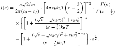
    (3.22)

• 4. Description:

  • Describes the speed/energy distribution of a particle at a particular angular direction.

  • The potential energy is ignored.

• 5. Usage:

  • Models the speed/energy distribution at a particular polar angle ϑ between u,u _b .

  • Estimates the expectation value of any function of the speed/energy, f(u), f(ε), which would be depended on the angular direction c≡cosϑ, i.e., 〈f(c)〉=∫f(u)⋅P _V(u,c)du=∫f(ε)⋅P _E(ε,c)dε.

• 6. Applications: Usually it is necessary to construct the kappa distribution of energies for a certain angular direction. For example, energetic neutral atoms generated from protons in the inner heliosheath may propagate in any direction from outward 0^∘ to directly back inward 180^∘, however, only the larger (oblique) angles can be detected back in the inner heliosphere.

3.6 Kappa Distribution of Speed/Energy over an Aperture

• 1. Tool Symbol: [UE].

• 2. Properties: 1-particle, 1-dimensional distribution. Variables: speed (velocity magnitude) or energy. Parameters: κ, θ, u _b (or ε _b ), aperture Δϑ×Δφ with ϑ ₀≤ϑ≤ϑ _f ≡ϑ ₀+Δϑ, φ ₀≤φ≤φ _f ≡φ ₀+Δφ (the polar angle ϑ is measured from the fixed flow direction of u _b (c ₀≡cosϑ ₀, s ₀≡sinϑ ₀, c _f ≡cosϑ _f , s _f ≡sinϑ _f ).

• 3. Formulation:

  • Speed:

    

    (3.23)

    with normalization $\int_{0}^{\infty} P_{\mathrm{V}}(u;c_{0},c_{f};u_{b};\theta,\kappa)du = 1$.

  • Energy:

    

    (3.24)

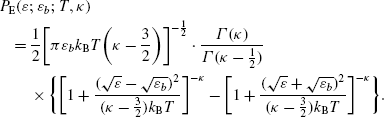
    with normalization $\int_{0}^{\infty} P_{\mathrm{E}}(\varepsilon ;c_{0},c_{f};\varepsilon _{b};T,\kappa)d\varepsilon= 1$, and

    

    (3.25)

  • Flux, averaged in the solid angle ΔΩ=Δφ(c ₀−c _f ):

    

    (3.26)

  Special cases:

  • (i) Total aperture (0^∘≤ϑ≤180^∘,0^∘≤φ≤360^∘; c ₀=1, c _f =−1):

    • Speed:

      

      (3.27)

    • Energy:

      

      (3.28)

    • Flux:

      

      (3.29)

  • (ii) If the flow speed is ignored, i.e., u _b ≪θ or ε _b ≪k _B T (e.g., inner heliosheath, planetary magnetosheath):

    • Speed:

      

      (3.30)

    • Energy:

      

      (3.31)

    • Flux:

      

      (3.32)

      The 1-particle kappa distribution of energy can be associated with the waiting time distributions of explosive events (Livadiotis and McComas 2013c).

  • (iii) Thermal Equilibrium, κ→∞ (Maxwellian distribution of velocities):

    • Speed:

      

      (3.33)

    • Energy:

      

      (3.34)

    • Flux:

      

      (3.35)

      where

      

      (3.36)
      

      (3.37)

• 4. Description:

  • Describes the speed/energy distribution of a particle over a certain aperture ΔΩ=Δφ(c ₀−c _f ).

  • The angles (ϑ,φ) have been integrated over their respective ranges, ϑ∈[ϑ ₀,ϑ _f ] or c∈[c _f ,c ₀], and φ∈[φ ₀,φ _f ].

  • The potential energy is ignored.

• 5. Usage:

  • Models the speed/energy distribution accumulated from all the angular directions within a given aperture.

  • Provides the expectation value of a function of speed/energy, f(u), f(ε), over all the angles, i.e., 〈f〉=∫f(u)⋅P _V(u)du=∫f(ε)⋅P _E(ε)dε.

• 6. Applications: This is useful when the distribution of speeds or energies is constructed by collecting measurements from all the angles within the given aperture. For example, the Solar Wind Around Pluto (SWAP) instrument onboard New Horizons (McComas et al. 2008) collects particles in an aperture 138^∘×10^∘ (ϑ ₀=0^∘, ϑ _f =138^∘, φ ₀=−5^∘, φ _f =5^∘). The distributions P _V(u;c ₀,c _f ,Δφ;u _b ;θ,κ) or P _E(ε;c ₀,c _f ,Δφ;ε _b ;T,κ) should be used for the respective data analyses. When the flow speed can be ignored, applications may be found in the inner heliosheath (e.g. Livadiotis et al. 2011, 2012, 2013), and the magnetosheath (e.g. Ogasawara et al. 2012).

3.7 Angular Kappa Distribution

• 1. Tool Symbol: [Ω].

• 2. Properties: 1-particle, 1-dimensional distribution; independent variables: angular direction ϑ, c≡cosϑ.

• 3. Formulation:

  

  (3.38)

  with x _f ≡ε _f /(k _B T), x ₀≡ε ₀/(k _B T), x _b ≡ε _b /(k _B T).

• 4. Description:

  • Describes the angular distribution of a particle when integrating over the energies ε ₀,ε _f .

  • The potential energy is ignored.

• 5. Usage:

  • Models the angular distribution, accumulated from all the energies.

  • Provides the expectation value of a function of ϑ, f(cosϑ), i.e., 〈f〉=∫f(c)⋅P(c)dc.

• 6. Applications: This is useful when the measurements are collected from some range of energy and restricted to a particular angle. For example, the angular distribution can be expressed in terms of the ecliptic coordinates if the relation between the angular direction ϑ and the ecliptic polar ϑ _E and azimuth φ _E angles is known.

4 Discussion–Conclusions

In this paper we (1) describe the physical underpinning of kappa distributions, which arise naturally from non-extensive Statistical Mechanics, (2) provide the basic formulae for kappa distributions, and (3) examine some applications of these distributions to space plasma research. In particular, seven main types of kappa distribution formulae were developed (see Appendix B for derivations) and discussed. These can be classified in three different ways: (i) N-particle or 1-particle distributions, (ii) distributions of Hamiltonian or of velocities, (iii) distributions of position/velocity vectors or of speed/energy/angles.

The complete and accurate form is the N-particle distribution of Hamiltonian; this can be reduced to the N-particle distribution of velocities when the potential energy is ignored. The same holds for the 1-particle distributions (of Hamiltonian and velocities). These are derived by integrating over the phase space of (N−1) particles. While the N-particle distributions are the exact formulae that must be used in some applications, the 1-particle distributions are more convenient and simpler to apply. For some cases, the 1-particle distributions are sufficiently accurate, and thus, the complications of the N-particle description are unnecessary. This applies when (1) we estimate the expectation values of functions of 1-particle velocity, f(u), e.g. statistical moments (f(u)=|u−u _b |^a); (2) the distribution and the system are homogeneous to all the velocity components of all the particles; hence, the N particles of d kinetic degrees of freedom each can be handled as one particle of f=N⋅d degrees of freedom; or (3) experimental measurements construct 1-particle distributions, hence, we need to deduce the analytical formulae of 1-particle distributions in order to compare with experimentally derived distributions. Table 3 summarizes the distributions of position/velocity vectors.

Table 3 Usage of distributions of velocities vectors

The last three tools (UEΩ, UE, Ω) correspond to formulae in which the velocity vector has been reduced to its magnitude (speed) or energy, and the angular direction. Tool UEΩ has both the speed/energy and the angular direction, and involves the speed/energy distributions at a certain angle ϑ. Tool UE corresponds to the distributions constructed after integrating over the angles (over an aperture ΔΩ=Δφ(c ₀−c _f )), while the tool Ω corresponds to the distribution constructed after integrating over the energies (over a certain energy range Δε). Table 4 summarizes distributions of speed/energy/angles. (The usage of the tools $1\vec{\mathrm{U}}$, UEΩ, and UE are summarized in Table 4 and illustrated in Fig. 6.)

Fig. 6

The most common formulations of the kappa distribution for direct use in space plasma analyses are (1) the three dimensional velocity vector (tool $1\vec{\mathrm{U}}$), (2) the speed/energy distribution for a particular Ω (tool UEΩ), and (3) the speed/energy distribution over the aperture ΔΩ (tool UE). The three cases have been respectively applied to the Ulysses ion/electron measurements, the IBEX ENA spectra, and the New Horizons fluxes of protons collected through an aperture of Δϑ=138^∘, Δφ=10^∘ (For references, see Table 4)

Table 4 Usage of distributions of speeds/energies/angles

The formulae developed and provided in this paper should be used for future space physics analyses that seek to apply kappa distributions in space data analysis, simulations, modeling, and other theoretical work. Using these equations guarantees results that remain firmly grounded on the foundation of non extensive statistical mechanics. Thus, this study provides a useful set of tools for the research in the field of space physics and astrophysics.

Appendices

Appendix A: Foundations of Non-extensive Statistical Mechanics

Non-extensive statistics generalizes (i) the classical formulation of Boltzmann-Gibbs entropy, and (ii) the notion of the canonical distribution via the formalism of escort probabilities. The ordinary p(u) and escort P(u) probability distributions are related to each other by the relations

$$ P(\boldsymbol{u}) = p(\boldsymbol{u})^{q}\Big/\int_{ - \infty} ^{\infty} p(\boldsymbol{u})^{q}d\boldsymbol{u} \Leftrightarrow p(\boldsymbol{u}) = P(\boldsymbol{u})^{1/q}\Big/\int _{ - \infty} ^{\infty} P(\boldsymbol{u})^{1/q}d\boldsymbol{u}. $$

(A.1)

For example, the mean (kinetic) energy (which equals the internal energy, U=〈ε〉) has different expressions for the ordinary

$$ U = \int_{ - \infty} ^{\infty} \biggl(\frac{1}{2}m\boldsymbol{u}^{2} \biggr) \cdot p(\boldsymbol{u})d\boldsymbol{u} $$

(A.2a)

and escort distributions

$$ U = \int_{ - \infty} ^{\infty} \biggl(\frac{1}{2}m\boldsymbol{u}^{2} \biggr) \cdot P(\boldsymbol{u})d\boldsymbol{u} = \frac{\int_{ - \infty} ^{\infty} (\frac{1}{2}m\boldsymbol{u}^{2}) \cdot p(\boldsymbol{u})^{q}d\boldsymbol{u}}{\int_{ - \infty} ^{\infty} p(\boldsymbol{u})^{q}d\boldsymbol{u}}. $$

(A.2b)

The non-extensive entropy is given by

$$ S_{q} = \frac{1}{q - 1} \cdot\biggl\{ {}1 - \int _{ - \infty} ^{\infty} \bigl[\delta u^{3}p(\boldsymbol{u}) \bigr]^{q - 1} \cdot p(\boldsymbol{u})d\boldsymbol{u} \biggr\} $$

(A.3a)

(where δu denotes a speed scale characterizing the system). Originally this was given in terms of the ordinary distribution, but it can be expressed also in terms of the escort distribution (Livadiotis and McComas 2011b),

$$ S_{q} = \frac{1 - \{ \int_{ - \infty} ^{\infty} [\delta u^{3}P(\boldsymbol{u})]^{1/q - 1} \cdot P(\boldsymbol{u})d\boldsymbol{u} \}^{ - q}}{q - 1}, $$

(A.3b)

where the BG entropy is recovered for q=1,

$$ S_{1} = - \int_{ - \infty} ^{\infty} \ln\bigl[ \delta u^{3}P(\boldsymbol{u})\bigr] \cdot P(\boldsymbol{u})d\boldsymbol{u}. $$

(A.3c)

The famous Gibbs path of entropy maximization involves maximizing the entropy under the Canonical ensemble’s constraints and deriving the canonical probability distribution. After its first presentation, the non-extensive entropy (Tsallis 1988) faced some fundamental problems (e.g., see Livadiotis 2009). In particular, the canonical distribution of energy ε was not invariant under arbitrary zero-level energy, while the internal energy U=〈ε〉 was not extensive as it should be for uncorrelated distributions. These inconsistencies as well as other problems were corrected by the later work of Tsallis et al. (1998). According to the old formalism of non-extensive statistics, the extremization of entropy in the Canonical ensemble was realized under the constraint of internal energy that was expressed in terms of the ordinary probability distribution (of energy p(ε) or velocity p(u)), instead of the escort one (that is P(ε)=p(ε)^q or P(u)∼p(u)^q). Then, the kappa distribution is derived by the transformation κ=−1/(q−1). On the other hand, a solid foundation for non extensive statistics (Tsallis et al. 1998), requires the expectation value to be given always in terms of the escort probability distribution, and thus, the same holds for the constraint of the internal energy in the Canonical Ensemble (see Appendix B in Livadiotis and McComas 2009). Namely, using the distribution of velocities,

$$ \langle f \rangle = \int_{ - \infty} ^{\infty} f(\boldsymbol{u}) \cdot P(\boldsymbol{u})d\boldsymbol{u} = \frac{\int_{ - \infty} ^{\infty} f(\boldsymbol{u}) \cdot p(\boldsymbol{u})^{q}d\boldsymbol{u}}{\int_{ - \infty} ^{\infty} p(\boldsymbol{u})^{q}d\boldsymbol{u}}. $$

(A.4)

Then, the derived Canonical probability distribution has the power exponent −1/(q−1), and now the correct transformation that leads to the kappa distribution is κ=1/(q−1).

In short:

• According to the old formalism of non-extensive statistics (Tsallis 1988) the canonical distribution is

  $$ p\biggl(\varepsilon= \frac{1}{2}m\boldsymbol{u}^{2}\biggr)\sim\biggl[ 1 + (1 - q) \cdot\frac{\varepsilon- U}{k_{\mathrm{B}}T_{\mathrm{L}}} \biggr]^{\frac{1}{q - 1}}\sim\biggl[ 1 + \frac{1}{\kappa} \cdot\frac{\varepsilon- U}{k_{\mathrm{B}}T_{\mathrm {L}}} \biggr]^{ - \kappa}. $$

  (A.5)

• According to the revised version of non-extensive statistics (Tsallis et al. 1998) the ordinary distribution is

  $$ p\biggl(\varepsilon= \frac{1}{2}m\boldsymbol{u}^{2}\biggr)\sim\biggl[ 1 + (q - 1) \cdot\frac{\varepsilon- U}{k_{\mathrm{B}}T_{\mathrm{phys}}} \biggr]^{ - \frac{1}{q - 1}}\sim \biggl[ 1 + \frac{1}{\kappa} \cdot\frac{\varepsilon- U}{k_{\mathrm{B}}T_{\mathrm {phys}}} \biggr]^{ - \kappa}. $$

  (A.6a)

However, the canonical distribution is given by the escort one

(A.6b)

(for the derivations, see Livadiotis and McComas 2009). The two formalisms, (A.5) and (A.6b), do not differ simply in the κ-exponents, and the sign of the transformation between the kappa and q indices. The most important difference is the temperature that is involved in the expressions of the distributions. In particular, in the old formalism, the derived probability distribution includes the Lagrangian temperature T _L (the one related with the second Lagrangian multiplier), while the new formalism contains the physical temperature T _phys, which it is the actual temperature for stationary systems out of thermal equilibrium.

Any probability distribution can be derived from the entropy maximization with a suitable choice of the constraint. This is possible even with BG entropy. For example, instead of constraining the mean energy, one could consider the mean logarithm of the energy. This was studied by Collier (2004), where the derived canonical-like distribution coincides with the kappa distribution. This is an elegant mathematical exercise. A physical foundation, however, requires the two classical constraints of the canonical ensemble: (i) the normalization of the distribution to unity, and (ii) the knowledge of the internal (mean) energy. Having these constraints, the extracted canonical probability distribution is unique and physically meaningful.

Note that the entropy can be directly defined in terms of the escort P (as in Eq. (A.3b), e.g. Livadiotis and McComas 2011b), which avoids the duality of ordinary/escort distributions. Because of the equivalency of q and κ, entropy can also be defined in terms of the kappa index κ≡1/(q−1), which is more popular in space physics,

$$ S_{\kappa} = \kappa- \kappa\cdot\biggl\{ \int_{ - \infty} ^{\infty} \bigl[\delta u^{3}P(\boldsymbol{u})\bigr]^{ - 1/(\kappa+ 1)} \cdot P(\boldsymbol{u})d\boldsymbol{u} \biggr\}^{ - 1 - 1/\kappa}, $$

(A.7a)

where the BG entropy is recovered for κ→∞.

It is worth mentioning that in all the above equations, the probability distributions, e.g. P(u), are not dimensionless. The respective dimensionless distributions must include the speed scale δu. For example, the distribution P(u) can be replaced by the dimensionless $\tilde{P}(\boldsymbol{u}) = P(\boldsymbol{u}) \cdot\delta u^{3}$ with normalization $\int_{ - \infty} ^{\infty} \tilde{P}(\boldsymbol{u})(d\boldsymbol{u} / \delta u^{3}) = 1$, where the ratio d u/δu ³ gives the number of states included in the interval [u,u+d u]. Then, the entropy is written as

$$ S_{\kappa} = \kappa- \kappa\cdot\biggl[ \int_{ - \infty} ^{\infty} \tilde{P}(\boldsymbol{u})^{\frac{\kappa}{\kappa+ 1}}\frac{d\boldsymbol{u}}{\delta u^{3}} \biggr]^{ - \frac{\kappa+ 1}{\kappa}}. $$

(A.7b)

More accurate, the entropy is given by the integration over the N-particle phase space

$$ S_{\kappa} = \kappa- \kappa\cdot\biggl[ \int_{ - \infty} ^{\infty} \tilde{P}(\boldsymbol{u})^{\frac{\kappa}{\kappa+ 1}}\frac{d\boldsymbol{u}_{1}d\boldsymbol{u}_{2} \cdots d\boldsymbol{u}_{N}}{\delta u^{3N}} \biggr]^{ - \frac{\kappa+ 1}{\kappa}}, $$

(A.7c)

with $\kappa= \kappa_{0} + \frac{3}{2}N$ (see Eq. (B.3) in Appendix B). The more general case is when the system is characterized by some potential energy Φ. Given the Hamiltonian, i.e., the sum of kinetic and potential energy, $H(\{ \boldsymbol{r}_{n}\},\{ \boldsymbol{u}_{n}\} ) = \frac {1}{2}m\sum_{n = 1}^{N} \boldsymbol{u}_{n}^{2} + \varPhi(\{ \boldsymbol{r}_{n}\} )$, the distribution of the Hamiltonian $\tilde{P}(H)$ is involved in the entropy as

(A.7d)

where σ is some characteristic phase space scale that is connected with the speed scale δu=σ/L through the system’s size scale L. (We have used the symbolism {r _n }=r ₁,r ₂,…,r _N and {u _n }=u ₁,u ₂,…,u _N .)

When the system is described by a discrete energy spectrum $\{ \varepsilon_{k}\} _{k = 1}^{W}$ associated with a discrete probability distribution $\{ p_{k}\} _{k = 1}^{W}$ (or $\{ P_{k}\} _{k = 1}^{W}$, with $P_{k} = p_{k}^{q}/\sum_{k' = 1}^{W} p_{k'}^{q} \Leftrightarrow p_{k} = P_{k}^{1/q}/\sum_{k' = 1}^{W} P_{k'}^{1/q}$, ∀k=1,…,W), then the non-extensive entropy is given by

$$ S_{q} = \frac{1}{q - 1} \cdot\Biggl( 1 - \sum _{k = 1}^{W} p_{k}^{q} \Biggr), $$

(A.8a)

$$ S_{q} = \frac{1}{q - 1} \cdot\Biggl[ 1 - \Biggl( \sum _{k = 1}^{W} P_{k}^{1/q} \Biggr)^{ - q} \Biggr], $$

(A.8b)

or in terms of the kappa index

$$ S_{\kappa} = \kappa\cdot\Biggl[ 1 - \Biggl( \sum _{k = 1}^{W} P_{k}^{\frac{\kappa}{\kappa+ 1}} \Biggr)^{ - \frac{\kappa+ 1}{\kappa}} \Biggr], $$

(A.8c)

leading to the BG formulation for κ→∞ (or q=1)

$$ S_{1} = - \sum_{k = 1}^{W} p_{k}\ln(p_{k}). $$

(A.8d)

(Note that all the above entropic formulations are given in units of the Boltzmann’s constant k _B.)

Non-extensive Statistical Mechanics involves a consistent and solid mathematical framework. In particular, the entropy fulfils all the required mathematical conditions (Tsallis 2009):

• (i) Non-negativity: The entropy is either positive or zero (when one of the possibilities equals unity).

• (ii) Maximization at equidistribution: S _κ is maximized when p _k =1/W, ∀k=1,…,W and κ>0.

• (iii) Non-additivity: Given two sets A and B of discrete distributions $\{ p_{i}^{A}\} _{i = 1}^{W}$ and $\{ p_{j}^{B}\} _{j = 1}^{W}$, then $S_{\kappa} (A + B) = S_{\kappa } (A) + S_{\kappa} (B) - \frac{1}{\kappa} \cdot S_{\kappa} (A)S_{\kappa} (B)$.

• (iv) Experimental Robustness: The entropy is stabilized under fluctuations of the relevant probability distribution (Abe 2002).

• (v) Uniqueness: It is the only entropic form that fulfills the generalized information measure (Santos 1997; Abe 2000). Non-extensive statistics have been studied in detail. Indeed, notions as such of the q-independence, the q-Fourier transformation and the relevant central theorem (Moyano et al. 2006; Umarov et al. 2008), the consistent q-generalization of basic statistical functions (Trigonometric and hyperbolic functions, Borges 1998; Gamma functions, Niven and Suyari 2009; Livadiotis and McComas 2009, etc.) and numerous other theorems and properties, lead to a well-established foundation of the non-extensive Statistical Mechanics.

The non-extensive formulation of entropy (A.7a)–(A.7d) is found to well describe many physical systems (Tsallis 2009), such as space plasmas (see introduction). However, it is possible that the actual entropy of the systems is not generally given by BG, Tsallis, or any other single entropy formulations. Rather, it may be that the actual entropy formulation S is a superposition of single entropy modes such as the Tsallis entropy, i.e., S=∑ _κ D(κ)S _κ , where D(κ) stands for the system’s density of kappa indices. Since the kappa index describes the correlations of the system (Livadiotis and McComas 2011b), then in general, the actual entropy of any system cannot be simply a Tsallis or any other universal formula, but has to be determined by the particular correlations of the particles of each system.

Let two sets A and B of discrete probability distributions be $\{ p_{i}^{A}\} _{i = 1}^{W}$ and $\{ p_{j}^{B}\} _{j = 1}^{W}$. BG Statistical Mechanics requires that there must be absolutely no correlation between the particles, i.e., $p_{ij}^{A + B} = p_{i}^{A} \cdot p_{j}^{B}$. Only then, the BG entropy is additive, i.e., S ^A+B=S ^A+S ^B. On the other hand, non-extensive Statistical Mechanics implies a certain type of correlation, that is $p_{ij}^{A + B} = g(p_{i}^{A},p_{j}^{B};a)$, where g(x,y;a)≡[x ^−a+y ^−a−1]^−1/a. Then, the BG entropy is non-additive, i.e., S ^A+B=S ^A+S ^B−a⋅S ^A⋅S ^B. Only Tsallis entropy is still additive, under this type of correlation. The a parameter is easily related to the kappa or q-index:q−1=1/κ≡a.

A generalized correlation function can be written as a superposition of correlations of the a-type, as soon as the system’s density of a or kappa (D(a) or D(κ)) is given. Therefore, starting from the dynamics of the systems it is possible to derive the correlation between the particles, $p_{ij}^{A + B} = f(p_{i}^{A},p_{j}^{B})$, and the function f is expressed in terms of a superposition of a-type correlation, f(x,y)=∑ _a D(a)g(x,y;a). The derivation of D(a) or D(κ) leads to the relevant superposition of the kappa distribution and the entropic function. We note that since the applied statistics is non-additive, then a non-additive rule must characterize the summation over kappa (or a) indices, generally written as f(x,y)=ϕ ⁻¹{∑ _a ϕ[D(a)g(x,y;a)]}, where ϕ is some monotonic function.

Clearly, there is not any single or absolute universal functional form for the entropy. On the contrary, the entropy is determined by the detailed particle dynamics of each system. The general characteristic is that the entropy can always be determined as a superposition of Tsallis entropy S _κ , the correlation as superposition of a-correlations, and the canonical probability distribution as superposition of kappa distributions (see spectral statistics in Tsallis 2009).

Appendix B: Construction of Kappa Distributions

The construction of a kappa distribution implies that the source distribution is isotropic in its fluid frame. This is true in the approximation that the energy of the system is given simply by the kinetic energy of the involved particles. In the general case, the kappa distribution concerns the distribution of the Hamiltonian H that can be reduced to the distribution of the velocities when H is given simply by the kinetic energy. A slight potential energy, e.g. the presence of an external magnetic field, can break the isotropy of the distribution in the fluid frame (see Livadiotis et al. 2013).

Given the Hamiltonian, $H(\{ \boldsymbol{r}_{n}\},\{ \boldsymbol{u}_{n}\} ) = \frac{1}{2}m\sum _{n = 1}^{N} \boldsymbol{u}_{n}^{2} + \varPhi (\{ \boldsymbol{r}_{n}\} )$, the phase space distribution is the kappa distribution of N particles (of d-degrees of freedom each),

$$ P\bigl(\{ \boldsymbol{r}_{n}\},\{ \boldsymbol{u}_{n}\};\kappa,T;N\bigr) \propto \biggl[ 1 + \frac{1}{\kappa_{0}} \cdot\frac{H(\{ \boldsymbol{r}_{n}\},\{ \boldsymbol{u}_{n}\} )}{k_{\mathrm{B}}T} \biggr]^{ - \kappa_{0} - 1 - \frac{d}{2}N}, $$

(B.1)

where the normalization (tool [NH]) is obtained by integrating over all the positions ∫d r ₁ d r ₂⋯d r _N and velocities ∫d u ₁ d u ₂⋯d u _N , i.e., ∫P({r _n },{u _n })d r ₁ d r ₂⋯d r _N d u ₁ d u ₂⋯d u _N =1. Assuming the particles have only kinetic energy, the N-particle kappa distribution is

(B.2)

where $\theta\equiv\sqrt{2k_{\mathrm{B}}T/m}$ is the temperature in speed dimensions; κ ₀ is the invariant kappa index (Livadiotis and McComas 2011b), which is independent of the kinetic degrees of freedom of the system (either per particle d or total f≡d⋅N), and it is connected to the dependent kappa index κ through the relation

$$ \kappa= \kappa_{0} + \frac{1}{2}d \cdot N. $$

(B.3)

In terms of the kinetic energy $\varepsilon= \frac{1}{2}m\sum_{n = 1}^{N} \boldsymbol{u}_{n}^{2}$, the distribution in Eq. (B.2) is written as

(B.4)

with $\int_{0}^{\infty} P_{\mathrm{E}}(\varepsilon;T;\kappa _{0};N)d\varepsilon= 1$. Figure 7 depicts the dimensionless distribution P _E(ε;T;κ ₀;N)⋅(k _B T) Eq. (B.4) in terms of the dimensionless energy ε⋅(k _B T)⁻¹, for various values of κ ₀ and number of particles N=1 and N=3. The inset in Fig. 7 shows the asymptotic behavior of Eq. (B.4) in the high energy limit, that is $P_{\mathrm{E}}(\varepsilon \gg \kappa_{0}k_{\mathrm{B}}T)\sim \varepsilon^{ - (2 + \kappa _{0})}$, i.e., the slope on a log-log scale depends only on κ ₀, |∂logP _E/∂logε|∼2+κ ₀. We observe that for larger number of particles or kappa index, the distribution shifts to larger energies.

Fig. 7

The kappa distribution of energy, Eq. (B.4), is depicted for various values of kappa κ ₀=0.5,1,2, and degrees of freedom f=3N, with N=1 and 3. The same distribution is depicted in the input panel for the high energy limit and on a log-log scale, where we observe that the slope depends only on κ ₀ (the lines of the same color correspond to the same κ ₀ and thus have the same slope)

The entire N-particle distribution function, either of velocities Eq. (B.2) or of energy Eq. (B.4), has the whole statistical information of the system. On the other hand, the 1-particle distribution constitutes the simplest way to study the phase-space distribution of particles, but this is an approximation of N-particle statistical description. Since kappa distributions are exclusively referred to the 1-particle statistical description, we develop the exact formulation of this function. By integrating over (N−1) particles, we derive the 1-particle kappa distribution, i.e.,

$$ P(\boldsymbol{u};\theta,\kappa_{0}) = \bigl(\pi\theta^{2}\kappa _{0}\bigr)^{ - \frac{d}{2}} \cdot\frac{\varGamma(\kappa _{0} + 1 + \frac{d}{2})}{\varGamma(\kappa_{0} + 1)} \cdot\biggl[ 1 + \frac{1}{\kappa_{0}} \cdot\frac{\boldsymbol{u}^{2}}{\theta^{2}} \biggr]^{ - \kappa_{0} - 1 - \frac{d}{2}}, $$

(B.5)

and for the usual dimensionality d=3, we have

$$ P(\boldsymbol{u};\theta,\kappa_{0}) = \bigl(\pi\theta^{2}\kappa _{0}\bigr)^{ - \frac{3}{2}} \cdot\frac{\varGamma(\kappa _{0} + 1 + \frac{3}{2})}{\varGamma(\kappa_{0} + 1)} \cdot\biggl[ 1 + \frac{1}{\kappa_{0}} \cdot\frac{\boldsymbol{u}^{2}}{\theta^{2}} \biggr]^{ - \kappa_{0} - 1 - \frac{3}{2}}. $$

(B.6)

Equation (B.3) is now written as $\kappa= \kappa_{0} + \frac {3}{2}$, and Eq. (B.6) is better known in terms of κ, i.e.,

$$ P(\boldsymbol{u};\theta,\kappa) = \biggl[\pi\theta^{2}\biggl(\kappa- \frac{3}{2}\biggr)\biggr]^{ - \frac{3}{2}} \cdot\frac{\varGamma (\kappa+ 1)}{\varGamma(\kappa- \frac{1}{2})} \cdot \biggl( 1 + \frac{1}{\kappa- \frac{3}{2}} \cdot\frac{\boldsymbol{u}^{2}}{\theta ^{2}} \biggr)^{ - \kappa- 1}. $$

(B.7)

When the velocity is given in the inertial reference frame or some frame other than the co-moving fluid frame, then Eq. (B.7) is written as

(B.8)

Analyzing the particle velocity u in its magnitude u=|u| and angle ϑ from the flow velocity u _b , we obtain

(B.9)

where c≡cosϑ, while the normalization is given by $\int_{ - 1}^{1} \int_{0}^{\infty} P(u,c;\theta,\kappa)du dc = 1$. This two-dimensional distribution of (u,c) is not so useful as can be the two marginal distributions. By integrating Eq. (B.9) over the angles ϑ∈[0^∘,180^∘] or c∈[−1,1], we obtain the distribution of the particle speed,

(B.10)

with normalizations $\int_{0}^{\infty} P(u;u_{b};\theta,\kappa)du = 1$. By integrating over an arbitrary aperture ϑ∈[ϑ ₀,ϑ _f ], or c∈[c _f ,c ₀], c ₀≡cosϑ ₀, c _f ≡cosϑ _f , we obtain Eq. (3.23) (tool [UE]).

The usage of Eqs. (B.9), (B.10) is as follows: When we record measurements of the particle speeds under specific angle ϑ (or c), i.e., ϑ _∗ (or c _∗), then Eq. (B.9) is suitable to describe the extracted distribution that is P(u,c=c _∗;u _b ;θ,κ). On the other hand, when the distribution of speeds is constructed by collecting speed measurements from all the angles, then Eq. (B.10) is suitable to describe the extracted distribution. Equations (B.9), (B.10) are written in terms of the kinetic energy in the inertial frame, $\varepsilon= \frac{1}{2}mu^{2}$, that is respectively,

(B.11)

with $\int_{ - 1}^{1} \int_{0}^{\infty} P_{\mathrm{E}}(\varepsilon ,c;\varepsilon_{b};\theta,\kappa )d\varepsilon dc = 1$, and

(B.12)

with $\int_{0}^{\infty} P_{\mathrm{E}}(\varepsilon;\varepsilon _{b};T,\kappa)d\varepsilon= 1$. Figure 8 plots Eq. (B.12) in terms of ε/(k _B T) for various κ-indices. As κ→1.5, the distribution is reduced to a type of delta function at ε=ε _b .

Fig. 8

The kappa distribution of energy ε, Eq. (B.12), depicted for bulk energy ε _b /(k _B T)=1 and various κ-indices; κ=100 (red solid)—that practically represents a Maxwell distribution, κ=3 (blue dot), κ=2 (green dash), κ=1.6 (magenta dash-dot), κ=1.51 (light blue solid), and κ=1.50001 (brown dash-dot) that approaches the smallest possible kappa, κ→1.5. At this limit the distribution behaves as delta function at ε=ε _b

In addition, by integrating Eq. (B.9) over all the speeds u∈[0,∞), we obtain the angular distribution

(B.13)

with $\int_{ - 1}^{1} P(c,x_{b};\kappa)dc = 1$, and $x_{b} \equiv u_{b}^{2}/\theta^{2} = \varepsilon_{b}/(k_{\mathrm{B}}T)$, where it is defined $f ( t;\kappa ) \equiv \int_{0}^{\infty} (1 + y^{2} - 2yt)^{ - \kappa- 1}y^{2}dy$.

Figure 9 shows that this distribution has “wings”; these are relatively large distribution values existing away from the mode at ϑ=0^∘. In Fig. 9(a,b) we plot Eq. (B.13) for x _b =5 and 0.5, respectively. We observe that the highest wings are obtained for a kappa distribution (κ<∞) when x _b >1, and a Maxwell distribution (κ→∞) when x _b ≤1. Specifically, the distribution value at ϑ=±180^∘ (wings) is plotted in Fig. 9(c) as a function of κ, and for various values of x _b >1 and x _b ≤1. For x _b >1, the maximum of the distribution is given for a certain κ that increases as x _b decreases; at the limit x _b →1, this kappa index becomes κ→∞, and remains the same for any x _b <1.

Fig. 9

The distribution of angular direction c≡cosϑ, Eq. (B.13), depicted (in units of 2π) for (a) x _b =5, (b) x _b =0.5, and for κ=2, κ→∞. (c) The distribution at ϑ=±180^∘ plotted as a function of κ, and for various values of x _b >1, and x _b ≤1

References

S. Abe, Axioms and uniqueness theorem for Tsallis entropy. Phys. Lett. A 271, 74–79 (2000)
S. Abe, General pseudoadditivity of composable entropy prescribed by the existence of equilibrium. Phys. Rev. E 63, 061105 (2001)
S. Abe, Stability of Tsallis entropy and instabilities of Rényi and normalized Tsallis entropies: a basis for q-exponential distributions. Phys. Rev. E 66, 046134 (2002)
M. Abramowitz, I.A. Stegun (eds.), Handbook of Mathematical Functions with Formulas, Graphs, and Mathematical Tables, 9th edn. (Dover, New York, 1972), p. 946
A.S. Bains, M. Tribeche, C.S. Ng, Dust-acoustic wave modulation in the presence of q-nonextensive electrons and/or ions in dusty plasma. Astrophys. Space Sci. 343, 621–628 (2013)
T.K. Baluku, M.A. Hellberg, I. Kourakis, N.S. Saini, Dust ion acoustic solitons in a plasma with kappa-distributed electrons. Phys. Plasmas 17, 053702 (2010)
S.J. Bame, D.J. McComas, B.L. Barraclough, J.L. Phillips, K.J. Sofaly, J.C. Chavez, B.E. Goldstein, R.K. Sakurai, Astron. Astrophys. Suppl. Ser. 92, 237 (1992)
E.P. Borges, On a q-generalization of circular and hyperbolic functions. J. Phys. A 31, 5281–5288 (1998)
E.P. Borges, C. Tsallis, G.F.J. Anãnõs, P.M.C. de Oliveira, Nonequilibrium probabilistic dynamics at the logistic map edge of chaos. Phys. Rev. Lett. 89, 254103 (2002)
M. Bzowski, M.A. Kubiak, E. Möbius et al., Neutral interstellar helium parameters based on ibex-lo observations and test particle calculations. Astrophys. J. Suppl. Ser. 198, 12 (2012)
K. Chotoo, N. Schwadron, G. Mason et al., The suprathermal seed population for corotating interaction region ions at 1 AU deduced from composition and spectra of H+, He++, and He+ observed by wind. J. Geophys. Res. 105, 23107–23122 (2000)
S.P. Christon, A comparison of the Mercury and Earth magnetospheres: electron measurements and substorm time scales. Icarus 71, 448–471 (1987)
R. Clausius, Sixth Memoir: On the Application of the Theorem of the Equivalence of Transformations to Interior Work (1862), p. 215
M.R. Collier, Are magnetospheric suprathermal particle distributions (κ functions) inconsistent with maximum entropy considerations? Adv. Space Res. 33, 2108–2112 (2004)
M.R. Collier, D.C. Hamilton, The relationship between kappa and temperature in energetic ion spectra at Jupiter. Geophys. Res. Lett. 22(3), 303–306 (1995)
M.A. Dayeh, M.I. Desai, J.R. Dwyer et al., Composition and spectral properties of the 1 AU quiet-time suprathermal ion population during solar cycle 23. Astrophys. J. 693, 1588–1600 (2009)
R.B. Decker, S.M. Krimigis, Voyager observations of low energy ions during solar cycle 23. Adv. Space Res. 32, 597–602 (2003)
R.B. Decker, S.M. Krimigis, E.C. Roelof et al., Voyager 1 in the foreshock, termination shock, and heliosheath. Science 309, 2020–2024 (2005)
M.I. Desai, G.M. Mason, M.E. Wiedenbeck et al., Spectral properties of heavy ions associated with the passage of interplanetary shocks at 1 AU. Astrophys. J. 611, 1156–1174 (2004)
K. Dialynas, S.M. Krimigis, D.G. Mitchell, D.C. Hamilton, N. Krupp, P.C. Brandt, Energetic ion spectral characteristics in the Saturnian magnetosphere using Cassini/MIMI measurements. J. Geophys. Res. 114, A01212 (2009)
P. Eslami, M. Mottaghizadeh, H.R. Pakzad, Nonplanar dust acoustic solitary waves in dusty plasmas with ions and electrons following a q-nonextensive distribution. Phys. Plasmas 18, 102303 (2011)
L.A. Fisk, G. Gloeckler, The common spectrum for accelerated ions in the quiet-time solar wind. Astrophys. J. Lett. 640, L79–L82 (2006)
M. Gell-Mann, C. Tsallis, Nonextensive Entropy: Interdisciplinary Applications (Oxford University Press, New York, 2004)
C.M. Hammond, W.C. Feldman, J.L. Phillips, B.E. Goldstein, A. Balogh, Solar wind double ion beams and the heliospheric current sheet. J. Geophys. Res. 100, 7881–7889 (1996)
A. Hasegawa, K. Mima, M. Duong-van, Plasma distribution function in a superthermal radiation field. Phys. Rev. Lett. 54(24), 2608–2610 (1985)
J. Heerikhuisen, N.V. Pogorelov, V. Florinski, G.P. Zank, J.A. Le Roux, The effects of a k-distribution in the heliosheath on the global heliosphere and ENA flux at 1 AU. Astrophys. J. 682, 679–689 (2008)
J. Heerikhuisen et al., Pick-up ions in the outer heliosheath: a possible mechanism for the interstellar boundary explorer ribbon. Astrophys. J. 708(2), L126–L130 (2010)
M.G. Kivelson, Serendipitous science from flybys of secondary targets: Galileo at Venus, Earth, and asteroids; Ulysses at Jupiter. Rev. Geophys. Suppl. 33, 565–575 (1995)
I. Kourakis, S. Sultana, M.A. Hellberg, Dynamical characteristics of solitary waves, shocks and envelope modes in kappa-distributed non-thermal plasmas: an overview. Plasma Phys. Control. Fusion 54, 124001 (2012)
J.A. Le Roux, G.M. Webb, A. Shalchi, G.P. Zank, A generalized nonlinear guiding center theory for the collisionless anomalous perpendicular diffusion of cosmic rays. Astrophys. J. 716, 671–692 (2010)
M.P. Leubner, Fundamental issues on kappa-distributions in space plasmas and interplanetary proton distributions. Phys. Plasmas 11, 1306–1308 (2004)
G. Livadiotis, Approach on Tsallis statistical interpretation of hydrogen-atom by adopting the generalized radial distribution function. J. Math. Chem. 45, 930–939 (2009)
G. Livadiotis, D.J. McComas, Beyond kappa distributions: exploiting Tsallis statistical mechanics in space plasmas. J. Geophys. Res., Atmos. 114, 11105 (2009)
G. Livadiotis, D.J. McComas, Exploring transitions of space plasmas out of equilibrium. Astrophys. J. 714, 971–987 (2010a)
G. Livadiotis, D.J. McComas, Measure of the departure of the q-metastable stationary states from equilibrium. Phys. Scr. 82, 035003 (2010b)
G. Livadiotis, D.J. McComas, in AIP Conf. Proc., Non-Equilibrium Stationary States in the Heliosphere: The Influence of Pick-up Ions, ed. by J. LeRoux, V. Florinski, G.P. Zank, A. Coates (AIP, Melville, 2010c), p. 70
G. Livadiotis, D.J. McComas, The influence of pick-up ions on space plasma distributions. Astrophys. J. 738, 64 (2011a)
G. Livadiotis, D.J. McComas, Invariant kappa distribution in space plasmas out of equilibrium. Astrophys. J. 741, 88 (2011b)
G. Livadiotis, D.J. McComas, Non-equilibrium thermodynamic processes: space plasmas and the inner heliosheath. Astrophys. J. 749, 11 (2012a)
G. Livadiotis, D.J. McComas, Near-equilibrium heliosphere—far-equilibrium heliosheath, SW-13, in AIP Conf. Proc., ed. by G.P. Zank, J. Spann (AIP, New York, 2012b in press)
G. Livadiotis, D.J. McComas, Fitting method based on correlation maximization: applications in astrophysics. J. Geophys. Res. (2013a in press)
G. Livadiotis, D.J. McComas, Entropy associated with the N-particle kappa distribution of non-equilibrium space plasmas (2013b in preparation)
G. Livadiotis, D.J. McComas, Evidence of large scale phase space quantization in plasmas. Entropy 15, 1116–1132 (2013c)
G. Livadiotis, D.J. McComas, M.A. Dayeh, H.O. Funsten, N.A. Schwadron, First sky map of the inner heliosheath temperature using IBEX spectra. Astrophys. J. 734, 1 (2011)
G. Livadiotis et al., Pick-up ion distributions and their influence on energetic neutral atom spectral curvature. Astrophys. J. 751, 64 (2012)
G. Livadiotis, D.J. McComas, N.A. Schwadron, H.O. Funsten, S.A. Fuselier, Pressure of the proton plasma in the inner heliosheath. Astrophys. J. 762, 134 (2013)
M. Maksimovic, I. Zouganelis, J.Y. Chaufray et al., Radial evolution of the electron distribution functions in the fast solar wind between 0.3 and 1.5 AU. J. Geophys. Res. 110, A09104 (2005)
G. Mann, H.T. Classen, E. Keppler, E.C. Roelof, On electron acceleration at CIR related shock waves. Astron. Astrophys. 391, 749–756 (2002)
E. Marsch, Kinetic physics of the solar corona and solar wind. Living Rev. Sol. Phys. 3, 1–100 (2006)
G.M. Mason et al., Abundances and energy spectra of corotating interaction region heavy ions observed during solar cycle 23. Astrophys. J. 678, 1458–1470 (2008)
B.H. Mauk, D.G. Mitchell, R.W. McEntire et al., Energetic ion characteristics and neutral gas interactions in Jupiter’s magnetosphere. J. Geophys. Res. 109, A09S12 (2004)
J.C. Maxwell, On the dynamical theory of gases. Philos. Mag. 32, 390–393 (1866)
D.J. McComas et al., The SolarWind Around Pluto (SWAP) instrument aboard new horizons. Space Sci. Rev. 140, 261–313 (2008)
D.J. McComas, F. Allegrini, P. Bochsler et al., IBEX–Interstellar Boundary Explorer. Space Sci. Rev. 146, 11–33 (2009a)
D.J. McComas, F. Allegrini, P. Bochsler et al., Global observations of the interstellar interaction from the Interstellar Boundary Explorer (IBEX). Science 326, 959–962 (2009b)
A.V. Milovanov, L.M. Zelenyi, Functional background of the Tsallis entropy: “coarse-grained” systems and “kappa” distribution functions. Nonlinear Process. Geophys. 7, 211–221 (2000)
L.G. Moyano, C. Tsallis, M. Gell-Mann, Numerical indications of a q-generalised central limit theorem. Europhys. Lett. 73(6), 813 (2006)
G. Nicolaou, D.J. McComas, F. Bagenal, H.A. Elliott, Fluid properties of plasma ions in the distant Jovian magnetosphere using Solar Wind Around Pluto (SWAP) data on new horizons, in AGU Fall-Meeting 2012, SM51A-2297 (2012)
R. Niven, H. Suyari, The q-gamma and (q,q)-polygamma functions of Tsallis statistics. Physica A 388, 4045–4060 (2009)
K. Ogasawara, V. Angelopoulos, M.A. Dayeh, S.A. Fuselier, G. Livadiotis, D.J. McComas, J.P. McFadden, Diagnosing dayside magnetosheath using energetic neutral atoms: IBEX and THEMIS observations. J. Geophys. Res. (2012 submitted)
V. Pierrard, M. Lazar, Kappa distributions: theory and applications in space plasmas. Sol. Phys. 267, 153–174 (2010)
M.A. Raadu, M. Shafiq, Test charge response for a dusty plasma with both grain size distribution and dynamical charging. Phys. Plasmas 14, 012105 (2007)
K. Roy, T. Saha, P. Chatterjee, M. Tribeche, Large amplitude double-layers in a dusty plasma with a q-nonextensive electron velocity distribution and two-temperature isothermal ions. Phys. Plasmas 19, 042113 (2012)
S. Saito, F.R.E. Forme, S.C. Buchert, S. Nozawa, R. Fujii, Effects of a kappa distribution function of electrons on incoherent scatter spectra. Ann. Geophys. 18, 1216–1223 (2000)
R.J.V. Santos, Generalization of Shannon’s theorem of Tsallis entropy. J. Math. Phys. 38(8), 4104–4107 (1997)
P. Schippers, M. Blanc, N. Andre et al., Multi-instrument analysis of electron populations in Saturn’s magnetosphere. J. Geophys. Res. 113, A07208 (2008)
N.A. Schwadron, F. Allegrini, M. Bzowski et al., Separation of the interstellar boundary explorer ribbon from globally distributed energetic neutral atom flux. Astrophys. J. 731, 56 (2011)
R.A. Treumann, Kinetic theoretical foundation of Lorentzian statistical mechanics. Phys. Scr. 59, 19–26 (1999)
M. Tribeche, M. Bacha, Nonlinear dust acoustic waves in a charge varying dusty plasma with suprathermal electrons. Phys. Plasmas 17, 073701 (2010)
M. Tribeche, A. Merriche, Nonextensive dust-acoustic solitary waves. Phys. Plasmas 18, 034502 (2011)
M. Tribeche, S. Mayout, R. Amour, Effect of ion suprathermality on arbitrary amplitude dust acoustic waves in a charge varying dusty plasma. Phys. Plasmas 16, 043706 (2009)
M. Tribeche, R. Amour, P.K. Shukla, Ion acoustic solitary waves in a plasma with nonthermal electrons featuring Tsallis distribution. Phys. Rev. E 85, 037401 (2012)
C. Tsallis, Possible generalization of Boltzmann-Gibbs statistics. J. Stat. Phys. 52, 479–487 (1988)
C. Tsallis, Introduction to Non-Extensive Statistical Mechanics: Approaching a Complex World (Springer, New York, 2009)
C. Tsallis, The nonadditive entropy SQ and its applications in physics and elsewhere: some remarks. Entropy 13, 1765–1804 (2011)
C. Tsallis, R.S. Mendes, A.R. Plastino, The role of constraints within generalized nonextensive statistics. Physica A 261, 534–554 (1998)
S. Umarov, C. Tsallis, S. Steinberg, A generalization of the central limit theorem consistent with nonextensive statistical mechanics. Milan J. Math. 76, 307–328 (2008)
V.M. Vasyliūnas, A survey of low-energy electrons in the evening sector of the magnetosphere with OGO 1 and OGO 3. J. Geophys. Res. 73, 2839–2884 (1968)
P.H. Yoon, Electron kappa distribution and steady-state Langmuir turbulence. Plasma Phys. 19, 052301 (2012)
P.H. Yoon, T. Rhee, C.M. Ryu, Self-consistent formation of electron κ distribution, 1: theory. J. Geophys. Res. 111, A09106 (2006)
G.P. Zank, J. Heerikhuisen, N.V. Pogorelov, R. Burrows, D.J. McComas, Microstructure of the heliospheric termination shock: implications for energetic neutral atom observations. Astrophys. J. 708, 1092 (2010)
I. Zouganelis, M. Maksimovic, N. Meyer-Vernet, H. Lamy, K. Issautier, A transonic collisionless model of the solar wind. Astrophys. J. 606, 542–554 (2004)
Acknowledgements
We are indebted to the space physics community that has been incorporating kappa distribution into their research progressively more over the past several decades, and for numerous comments and feedback on our analyses of these distributions over the past five years. This work was supported in part by a variety of NASA missions including ACE, IBEX, New Horizons, and Ulysses (ESA/NASA).
Author information
Authors and Affiliations
Corresponding author