
Abstract
In this chapter, we present the physical and physiological basics behind EEG and MEG signal generation and propagation. We first start by presenting the biophysical principles that explain how the coordinated movements of ions inside and outside neuronal cells result in macroscale phenomena at the scalp, such as electric potentials recorded by EEG and magnetic fields sensed by MEG. These physical principles enforce EEG and MEG signals to have specific spatial and temporal features, which can be used to study brain’s response to internal and external stimuli. We continue our exploration by developing a mathematical framework within which EEG and MEG signals can be computed if the distribution of underlying brain sources is known, a process called forward problem. We further continue to discuss methods that attempt the reverse, i.e., solving for underlying brain sources given scalp measurements such as EEG and MEG, a process called source imaging. We will provide various examples of how electrophysiological source imaging techniques can help study the brain during its normal and pathological states. We will also briefly discuss how combining electrophysiological signals from EEG with hemodynamic signals from functional magnetic resonance imaging (fMRI) helps improve the spatiotemporal resolution of estimates of the underlying brain sources, which is critical for studying spatiotemporal processes within the brain. The goal of this chapter is to provide proper physical and physiological intuition and biophysical principles that explain EEG/MEG signal generation, its propagation from sources in the brain to EEG/MEG sensors, and how this process can be inverted using signal processing and machine learning techniques and algorithms.
Access this chapter
Tax calculation will be finalised at checkout
Purchases are for personal use only
References
R. Caton, The electric currents of the brain. Br. Med. J. 2, 278 (1875)
H. Berger, Über das Elektrenkephalogramm des Menschen. Archiv f. Psychiatrie 87(1), 527–570 (1929). https://doi.org/10.1007/BF01797193
D. Cohen, Magnetoencephalography: Detection of the brain’s electrical activity with a superconducting magnetometer. Science 175(4022), 664–666 (1972). https://doi.org/10.1126/science.175.4022.664
B. He, A. Sohrabpour, E. Brown, Z. Liu, Electrophysiological source imaging: A noninvasive window to brain dynamics. Annu. Rev. Biomed. Eng. 20(1), 171–196 (2018)
B. Pesaran, M. Vinck, G.T. Einevoll, A. Sirota, P. Fries, M. Siegel, W. Truccolo, C.E. Schroder, R. Srinivasan, Investigating large-scale brain dynamics using field potential recordings: analysis and interpretation. Nat. Neurosci. 21(7), 903 (2018). https://doi.org/10.1038/s41593-018-0171-8
F.H. Lopes da Silva, EEG and MEG: Relevance to neuroscience. Neuron 80(5), 1112–1128 (2013). https://doi.org/10.1016/j.neuron.2013.10.017
M.S. Hämäläinen, R. Hari, R.J. Ilmoniemi, J. Knuutila, O.V. Lounasmaa, Magnetoencephalography—theory, instrumentation, and applications to noninvasive studies of the working human brain. Rev Mod. Phys. 65(2), 413 (1993)
J. Malmivuo, R. Plonsey, Bioelectromagnetism: Principles and Applications of Bioelectric and Biomagnetic Fields (Oxford University Press, New York, Oxford, 1995)
P.L. Nunez, R. Srinivasan, Electric Fields of the Brain: The Neurophysics of EEG (Oxford University Press, New York, 2006)
A. Sohrabpour, Y. Lu, P. Kankirawatana, J. Blount, H. Kim, B. He, Effect of EEG electrode number on epileptic source localization in pediatric patients. Clin. Neurophysiol. 126(3), 472–480 (2015)
M. Seeck, L. Koessler, T. Bast, F. Leijten, C. Michel, C. Baumgartner, B. He, S. Beniczky, The standardized EEG electrode array of the IFCN. Clin. Neurophysiol. 128, 2070 (2017)
G.A. Worrell, A.B. Gardner, S.M. Stead, S. Hu, S. Goerss, G.J. Cascino, F.B. Meyer, R. Marsh, B. Litt, High-frequency oscillations in human temporal lobe: Simultaneous microwire and clinical macroelectrode recordings. Brain 131(4), 928–937 (2008)
G. Buzsáki, F. Lopes da Silva, High frequency oscillations in the intact brain. Prog. Neurobiol. 98(3), 241–249 (2012). https://doi.org/10.1016/j.pneurobio.2012.02.004
J.D. Jirsch, E. Urrestarazu, P. LeVan, A. Olivier, F. Dubeau, J. Gotman, High-frequency oscillations during human focal seizures. Brain 129(6), 1593–1608 (2006)
Y. Lu, G.A. Worrell, H.C. Zhang, L. Yang, B. Brinkmann, C. Nelson, B. He, Noninvasive imaging of the high frequency brain activity in focal epilepsy patients. IEEE Trans. Biomed. Eng. 61(6), 1660–1667 (2014)
N. von Ellenrieder, L.P. Andrade-Valença, F. Dubeau, J. Gotman, Automatic detection of fast oscillations (40–200Hz) in scalp EEG recordings. Clin. Neurophysiol. 123(4), 670–680 (2012). https://doi.org/10.1016/j.clinph.2011.07.050
J. Jacobs, M. Zijlmans, R. Zelmann, C.E. Chatillon, J. Hall, A. Olivier, F. Dubeau, J. Gotman, High-frequency electroencephalographic oscillations correlate with outcome of epilepsy surgery. Ann. Neurol. 67(2), 209–220 (2010)
S.V. Gliske, Z.T. Irwin, C. Chestek, G.L. Hegeman, B. Brinkmann, O. Sagher, H.J.L. Garton, G.A. Worrell, W. Stacey, Variability in the location of high frequency oscillations during prolonged intracranial EEG recordings. Nat. Commun. 9(1), 2155 (2018). https://doi.org/10.1038/s41467-018-04549-2
E. Boto, N. Holmes, J. Leggett, G. Roberts, V. Shah, S.S. Meyer, L.D. Munoz, K.J. Mullinger, T.M. Tierney, S. Bestmann, G.R. Barnes, R. Bowtell, M.J. Brookes, Moving magnetoencephalography towards real-world applications with a wearable system. Nature 555(7698), 657–661 (2018). https://doi.org/10.1038/nature26147
R. Hari et al., IFCN-endorsed practical guidelines for clinical magnetoencephalography (MEG). Clin. Neurophysiol. 129(8), 1720–1747 (2018). https://doi.org/10.1016/j.clinph.2018.03.042
A. Gevins, J. Le, N.K. Martin, P. Brickett, J. Desmond, B. Reutter, High resolution EEG: 124-channel recording, spatial deblurring and MRI integration methods. Electroencephalogr. Clin. Neurophysiol. 90(5), 337–358 (1994). https://doi.org/10.1016/0013-4694(94)90050-7
P. Zhang, K. Jamison, S. Engel, B. He, S. He, Binocular rivalry requires visual attention. Neuron 71(2), 362–369 (2011)
B.M. Savers, H.A. Beagley, W.R. Henshall, The mechanism of auditory evoked EEG responses. Nature 247(5441), 481 (1974). https://doi.org/10.1038/247481a0
B. He, J. Lian, G. Li, High-resolution EEG: A new realistic geometry spline Laplacian estimation technique. Clin. Neurophysiol. 112(5), 845–852 (2001). https://doi.org/10.1016/S1388-2457(00)00546-0
A. Hillebrand, G.R. Barnes, A quantitative assessment of the sensitivity of whole-head MEG to activity in the adult human cortex. NeuroImage 16(3, Part A), 638–650 (2002). https://doi.org/10.1006/nimg.2002.1102
S. Baillet, Magnetoencephalography for brain electrophysiology and imaging. Nat. Neurosci. 20(3), 327–339 (2017)
M. Seeber, L.-M. Cantonas, M. Hoevels, T. Sesia, V. Visser-Vandewalle, C.M. Michel, Subcortical electrophysiological activity is detectable with high-density EEG source imaging. Nat. Commun. 10(1), 753 (2019). https://doi.org/10.1038/s41467-019-08725-w
F. Pizzo, N. Roehri, S.M. Villalon, A. Trebuchon, S. Chen, S. Lagarde, R. Carron, M. Gavaret, B. Giusiano, A. McGonigal, F. Bartolomei, J.M. Badier, C.G. Benar, Deep brain activities can be detected with magnetoencephalography. Nat. Commun. 10(1), 971 (2019). https://doi.org/10.1038/s41467-019-08665-5
F. Perrin, O. Bertrand, J. Pernier, Scalp current density mapping: Value and estimation from potential data. IEEE Trans. Biomed. Eng. BME-34(4), 283–288 (1987). https://doi.org/10.1109/TBME.1987.326089
B. He, R.J. Cohen, Body surface Laplacian ECG mapping. IEEE Trans. Biomed. Eng. 39(11), 1179–1191 (1992). https://doi.org/10.1109/10.168684
B. Hjorth, An on-line transformation of EEG scalp potentials into orthogonal source derivations. Electroencephalogr. Clin. Neurophysiol. 39(5), 526–530 (1975). https://doi.org/10.1016/0013-4694(75)90056-5
F. Babiloni, C. Babiloni, F. Carducci, L. Fattorini, P. Onorati, A. Urbano, Spline Laplacian estimate of EEG potentials over a realistic magnetic resonance-constructed scalp surface model. Electroencephalogr. Clin. Neurophysiol. 98(4), 363–373 (1996). https://doi.org/10.1016/0013-4694(96)00284-2
W. Besio, T. Chen, Tripolar Laplacian electrocardiogram and moment of activation isochronal mapping. Physiol. Meas. 28(5), 515–529 (2007). https://doi.org/10.1088/0967-3334/28/5/006
J.V. Haxby, A.C. Connolly, J.S. Guntupalli, Decoding neural representational spaces using multivariate pattern analysis. Annu. Rev. Neurosci. 37(1), 435–456 (2014). https://doi.org/10.1146/annurev-neuro-062012-170325
J. Linde-Domingo, M.S. Treder, C. Kerrén, M. Wimber, Evidence that neural information flow is reversed between object perception and object reconstruction from memory. Nat. Commun. 10(1), 179 (2019). https://doi.org/10.1038/s41467-018-08080-2
B. Gohel, S. Lim, M.-Y. Kim, H. Kwon, K. Kim, Dynamic pattern decoding of source-reconstructed MEG or EEG data: Perspective of multivariate pattern analysis and signal leakage. Comput. Biol. Med. 93, 106–116 (Feb. 2018). https://doi.org/10.1016/j.compbiomed.2017.12.020
R. Plonsey, Bioelectric Phenomena (Wiley Online Library, 1969). http://onlinelibrary.wiley.com/doi/10.1002/047134608X.W1403/full
B. He, T. Musha, Y. Okamoto, S. Homma, Y. Nakajima, T. Sato, Electric dipole tracing in the brain by means of the boundary element method and its accuracy. IEEE Trans. Biomed. Eng. 34(6), 406–414 (1987)
M.S. Hämäläinen, Interpreting Measured Magnetic Fields of the Brain: Estimates of Current Distributions (Helsinki University of Technology, Otaniemi, 1984)
A.M. Dale, M.I. Sereno, Improved localizadon of cortical activity by combining EEG and MEG with MRI cortical surface reconstruction: A linear approach. J. Cogn. Neurosci. 5(2), 162–176 (1993)
R.D. Pascual-Marqui, C.M. Michel, D. Lehmann, Low resolution electromagnetic tomography: A new method for localizing electrical activity in the brain. Int. J. Psychophysiol. 18(1), 49–65 (1994)
B. He, X. Zhang, J. Lian, H. Sasaki, D. Wu, V.L. Towle, Boundary element method-based cortical potential imaging of somatosensory evoked potentials using subjects’ magnetic resonance images. NeuroImage 16(3, Part A), 564–576 (2002). https://doi.org/10.1006/nimg.2002.1127
R.G. de Peralta Menendez, S.L.G. Andino, S. Morand, C.M. Michel, T. Landis, Imaging the electrical activity of the brain: ELECTRA. Hum. Brain Mapp. 9(1), 1–12 (2000)
S. Rush, D.A. Driscoll, EEG electrode sensitivity-an application of reciprocity. IEEE Trans. Biomed. Eng. BME-16(1), 15–22 (1969). https://doi.org/10.1109/TBME.1969.4502598
M.S. Hämäläinen, J. Sarvas, Realistic conductivity geometry model of the human head for interpretation of neuromagnetic data. IEEE Trans. Biomed. Eng. 36(2), 165–171 (1989)
J.C. Mosher, R.M. Leahy, P.S. Lewis, EEG and MEG: Forward solutions for inverse methods. IEEE Trans. Biomed. Eng. 46(3), 245–259 (1999)
Y. Yan, P.L. Nunez, R.T. Hart, Finite-element model of the human head: Scalp potentials due to dipole sources. Med. Biol. Eng. Comput. 29(5), 475–481 (1991)
Y. Zhang, L. Ding, W. van Drongelen, K. Hecox, D.M. Frim, B. He, A cortical potential imaging study from simultaneous extra- and intracranial electrical recordings by means of the finite element method. NeuroImage 31(4), 1513–1524 (2006). https://doi.org/10.1016/j.neuroimage.2006.02.027
C.H. Wolters, A. Anwander, X. Tricoche, D. Weinstein, M.A. Koch, R.S. MacLeod, Influence of tissue conductivity anisotropy on EEG/MEG field and return current computation in a realistic head model: A simulation and visualization study using high-resolution finite element modeling. NeuroImage 30(3), 813–826 (2006). https://doi.org/10.1016/j.neuroimage.2005.10.014
W.H. Lee, Z. Liu, B.A. Mueller, K. Lim, B. He, Influence of white matter anisotropic conductivity on EEG source localization: Comparison to fMRI in human primary visual cortex. Clin. Neurophysiol. 120(12), 2071–2081 (2009)
R.M. Gulrajani, Bioelectricity and Biomagnetism (New York, Wiley, 1998)
A.M. Dale, A.K. Liu, B.R. Fischl, R.L. Buckner, J.W. Belliveau, J.D. Lewine, E. Halgren, Dynamic statistical parametric mapping: Combining fMRI and MEG for high-resolution imaging of cortical activity. Neuron 26(1), 55–67 (2000)
Z. Liu, B. He, fMRI–EEG integrated cortical source imaging by use of time-variant spatial constraints. NeuroImage 39(3), 1198–1214 (2008)
B. He, Z. Liu, Multimodal functional neuroimaging: Integrating functional MRI and EEG/MEG. IEEE Rev. Biomed. Eng. 1, 23–40 (2008). https://doi.org/10.1109/RBME.2008.2008233
T. Musha, Y. Okamoto, Forward and inverse problems of EEG dipole localization. Crit. Rev. Biomed. Eng. 27(3–5), 189–239 (1999)
M. Scherg, D. Von Cramon, Two bilateral sources of the late AEP as identified by a spatio-temporal dipole model. Electroencephalogr. Clin. Neurophysiol./Evoked Potentials Sect. 62(1), 32–44 (1985)
H. Stefan, C. Hummel, G. Scheler, A. Genow, K. Druschky, C. Tilz, M. Kaltenhauser, R. Hopfengartner, M. Buchfelder, J. Romstock, Magnetic brain source imaging of focal epileptic activity: A synopsis of 455 cases. Brain 126(11), 2396–2405 (2003). https://doi.org/10.1093/brain/awg239
K. Kaiboriboon, S. Nagarajan, M. Mantle, H.E. Kirsch, Interictal MEG/MSI in intractable mesial temporal lobe epilepsy: Spike yield and characterization. Clin. Neurophysiol. 121(3), 325–331 (2010). https://doi.org/10.1016/j.clinph.2009.12.001
D. Cohen, B.N. Cuffin, A method for combining MEG and EEG to determine the sources. Phys. Med. Biol. 32(1), 85–89 (1987). https://doi.org/10.1088/0031-9155/32/1/013
M. Fuchs, M. Wagner, H.A. Wischmann, T. Kohler, A. Theiben, R. Drenckhahn, H. Buchner, Improving source reconstructions by combining bioelectric and biomagnetic data. Electroencephalogr. Clin. Neurophysiol. 107(2), 93–111 (1998). https://doi.org/10.1016/S0013-4694(98)00046-7
J.C. Mosher, P.S. Lewis, R.M. Leahy, Multiple dipole modeling and localization from spatio-temporal MEG data. IEEE Trans. Biomed. Eng. 39(6), 541–557 (1992)
B.D. Van Veen, W. Van Drongelen, M. Yuchtman, A. Suzuki, Localization of brain electrical activity via linearly constrained minimum variance spatial filtering. IEEE Trans. Biomed. Eng. 44(9), 867–880 (1997)
F. Babiloni, C. Babiloni, F. Carducci, L. Fattorini, C. Anello, P. Onorati, A. Urbano, High resolution EEG: A new model-dependent spatial deblurring method using a realistically-shaped MR-constructed subject’s head model. Electroencephalogr. Clin. Neurophysiol. 102(2), 69–80 (1997). https://doi.org/10.1016/S0921-884X(96)96508-X
Y. Lai, X. Zhang, W. van Drongelen, M. Kohrman, K. Hecox, Y. Ni, B. He, Noninvasive cortical imaging of epileptiform activities from interictal spikes in pediatric patients. NeuroImage 54(1), 244–252 (2011)
F. Babiloni, F. Cincotti, C. Babiloni, F. Carducci, D. Mattia, L. Astolfi, A. Basilisco, P.M. Rossini, L. Ding, Y. Ni, B. He, Estimation of the cortical functional connectivity with the multimodal integration of high-resolution EEG and fMRI data by directed transfer function. NeuroImage 24(1), 118–131 (2005)
C. Grova, J. Daunizeau, J.-M. Lina, C.G. Bénar, H. Benali, J. Gotman, Evaluation of EEG localization methods using realistic simulations of interictal spikes. NeuroImage 29(3), 734–753 (2006)
L. Ding, H. Yuan, Simultaneous EEG and MEG source reconstruction in sparse electromagnetic source imaging. Hum. Brain Mapp. 34(4), 775–795 (2013). https://doi.org/10.1002/hbm.21473
U. Mitzdorf, Current source-density method and application in cat cerebral cortex: Investigation of evoked potentials and EEG phenomena. Physiol. Rev. 65(1), 37–100 (1985). https://doi.org/10.1152/physrev.1985.65.1.37
J.-Z. Wang, S.J. Williamson, L. Kaufman, Magnetic source images determined by a lead-field analysis: The unique minimum-norm least-squares estimation. IEEE Trans. Biomed. Eng. 39(7), 665–675 (1992)
E. Biglieri, K. Yao, Some properties of singular value decomposition and their applications to digital signal processing. Signal Process. 18(3), 277–289 (1989). https://doi.org/10.1016/0165-1684(89)90039-X
Y. Shim, Z. Cho, SVD pseudoinversion image reconstruction. IEEE Trans. Acoust. Speech Signal Process. 29(4), 904–909 (1981). https://doi.org/10.1109/TASSP.1981.1163632
A.N. Tikhonov, V.Y. Arsenin, Solutions of Ill-Posed Problems (Wiley, New York, 1977)
V.A. Morozov, Methods for Solving Incorrectly Posed Problems (Springer Science & Business Media, Berlin, 1984)
P.C. Hansen, Analysis of discrete ill-posed problems by means of the L-curve. SIAM Rev. 34(4), 561–580 (1992)
P.C. Hansen, D.P. O’Leary, The use of the L-curve in the regularization of discrete ill-posed problems. SIAM J. Sci. Comput. 14(6), 1487–1503 (1993)
B. Jeffs, R. Leahy, M. Singh, An evaluation of methods for neuromagnetic image reconstruction. IEEE Trans. Biomed. Eng. BME-34(9), 713–723 (1987). https://doi.org/10.1109/TBME.1987.325996
G.H. Golub, M. Heath, G. Wahba, Generalized cross-validation as a method for choosing a good ridge parameter. Technometrics 21(2), 215–223 (1979). https://doi.org/10.1080/00401706.1979.10489751
S. Baillet, J.C. Mosher, R.M. Leahy, Electromagnetic brain mapping. IEEE Signal Process. Mag. 18(6), 14–30 (2001)
J. Daunizeau, J. Mattout, D. Clonda, B. Goulard, H. Benali, J. Lina, Bayesian spatio-temporal approach for EEG source reconstruction: Conciliating ECD and distributed models. IEEE Trans. Biomed. Eng. 53(3), 503–516 (2006). https://doi.org/10.1109/TBME.2005.869791
M. Zhu, W. Zhang, D.L. Dickens, L. Ding, Reconstructing spatially extended brain sources via enforcing multiple transform sparseness. NeuroImage 86, 280–293 (2014)
A. Sohrabpour, Y. Lu, G. Worrell, B. He, Imaging brain source extent from EEG/MEG by means of an iteratively reweighted edge sparsity minimization (IRES) strategy. NeuroImage 142, 27–42 (2016)
K. Sekihara, S.S. Nagarajan, Electromagnetic Brain Imaging: A Bayesian Perspective (Springer, Cham, 2015)
I.F. Gorodnitsky, J.S. George, B.D. Rao, Neuromagnetic source imaging with FOCUSS: A recursive weighted minimum norm algorithm. Electroencephalogr. Clin. Neurophysiol. 95(4), 231–251 (1995). https://doi.org/10.1016/0013-4694(95)00107-A
R. Pascual-Marqui, LORETA (Low Resolution Brain Electromagnetic Tomography): New authentic 3D functional Images of the brain. ISBET Newslett. Issue 5, 4–8 (1994)
L. Yang, C. Wilke, B. Brinkmann, G.A. Worrell, B. He, Dynamic imaging of ictal oscillations using non-invasive high-resolution EEG. NeuroImage 56(4), 1908–1917 (2011)
Y. Zhang, W. van Drongelen, M. Kohrman, B. He, Three-dimensional brain current source reconstruction from intra-cranial ECoG recordings. NeuroImage 42(2), 683–695 (2008). https://doi.org/10.1016/j.neuroimage.2008.04.263
V. Caune, R. Ranta, S. Le Cam, J. Hofmanis, L. Maillard, L. Koessler, V. Louis-Dorr, Evaluating dipolar source localization feasibility from intracerebral SEEG recordings. NeuroImage 98, 118–133 (2014). https://doi.org/10.1016/j.neuroimage.2014.04.058
S.A.H. Hosseini, A. Sohrabpour, B. He, Electromagnetic source imaging using simultaneous scalp EEG and intracranial EEG: An emerging tool for interacting with pathological brain networks. Clin. Neurophysiol. 129(1), 168–187 (2018)
K. Matsuura, Y. Okabe, A robust reconstruction of sparse biomagnetic sources. IEEE Trans. Biomed. Eng. 44(8), 720–726 (1997). https://doi.org/10.1109/10.605428
K. Matsuura, Y. Okabe, Selective minimum-norm solution of the biomagnetic inverse problem. IEEE Trans. Biomed. Eng. 42(6), 608–615 (1995)
K. Uutela, M.S. Hämäläinen, E. Somersalo, Visualization of magnetoencephalographic data using minimum current estimates. NeuroImage 10(2), 173–180 (1999)
M.X. Huang, A.M. Dale, T. Song, E. Halgren, D.L. Harrington, I. Podogorny, J.M. Canive, S. Lewis, R.R. Lee, Vector-based spatial–Temporal minimum L1-norm solution for MEG. NeuroImage 31(3), 1025–1037 (2006)
L. Ding, B. He, Sparse source imaging in electroencephalography with accurate field modeling. Hum. Brain Mapp. 29(9), 1053–1067 (2008)
M. Fuchs, M. Wagner, T. Köhler, H.-A. Wischmann, Linear and nonlinear current density reconstructions. J. Clin. Neurophysiol. 16(3), 267–295 (1999)
D. Wipf, S. Nagarajan, Iterative reweighted ℓ 1 and ℓ 2 methods for finding sparse solutions. IEEE J. Sel. Topics Signal Process. 4(2), 317–329 (2010)
K. Liao, M. Zhu, L. Ding, S. Valette, W. Zhang, D. Dickens, Sparse imaging of cortical electrical current densities via wavelet transforms. Phys. Med. Biol. 57(21), 6881 (2012). https://doi.org/10.1088/0031-9155/57/21/6881
K. Liao, M. Zhu, L. Ding, A new wavelet transform to sparsely represent cortical current densities for EEG/MEG inverse problems. Comput. Methods Prog. Biomed. 111(2), 376–388 (2013). https://doi.org/10.1016/j.cmpb.2013.04.015
L. Ding, Reconstructing cortical current density by exploring sparseness in the transform domain. Phys. Med. Biol. 54(9), 2683 (2009)
L. Ding, Y. Ni, J. Sweeney, B. He, Sparse cortical current density imaging in motor potentials induced by finger movement. J. Neural Eng. 8(3), 036008 (2011). https://doi.org/10.1088/1741-2560/8/3/036008
M. Zhu, W. Zhang, D.L. Dickens, J.A. King, L. Ding, Sparse MEG source imaging for reconstructing dynamic sources of interictal spikes in partial epilepsy. J. Clin. Neurophysiol. 30(4), 313–328 (2013). https://doi.org/10.1097/WNP.0b013e31829dda27
R.N. Henson, Y. Goshen-Gottstein, T. Ganel, L.J. Otten, A. Quayle, M.D. Rugg, Electrophysiological and haemodynamic correlates of face perception, recognition and priming. Cereb. Cortex 13(7), 793–805 (2003). https://doi.org/10.1093/cercor/13.7.793
D. Yao, B. He, A self-coherence enhancement algorithm and its application to enhancing three-dimensional source estimation from EEGs. Ann. Biomed. Eng. 29(11), 1019–1027 (2001)
K. Liu, Z.L. Yu, W. Wu, Z. Gu, Y. Li, S. Nagarajan, Variation sparse source imaging based on conditional mean for electromagnetic extended sources. Neurocomputing 313, 96 (2018). https://doi.org/10.1016/j.neucom.2018.06.004
A. Gramfort, D. Strohmeier, J. Haueisen, M.S. Hämäläinen, M. Kowalski, Time-frequency mixed-norm estimates: Sparse M/EEG imaging with non-stationary source activations. NeuroImage 70, 410–422 (2013)
B. He, L. Yang, C. Wilke, H. Yuan, Electrophysiological imaging of brain activity and connectivity—Challenges and opportunities. IEEE Trans. Biomed. Eng. 58(7), 1918–1931 (2011)
S. Ogawa, D.W. Tank, R. Menon, J.M. Ellermann, S.G. Kim, H. Merkle, K. Ugurbil, Intrinsic signal changes accompanying sensory stimulation: Functional brain mapping with magnetic resonance imaging. PNAS 89(13), 5951–5955 (1992)
K.K. Kwong, J.W. Belliveau, D.A. Chesler, I.E. Goldberg, R.M. Weisskoff, B.P. Poncelet, D.N. Kennedy, B.E. Hoppel, M.S. Cohen, R. Turner, Dynamic magnetic resonance imaging of human brain activity during primary sensory stimulation. PNAS 89(12), 5675–5679 (1992). https://doi.org/10.1073/pnas.89.12.5675
P.A. Bandettini, E.C. Wong, R.S. Hinks, R.S. Tikofsky, J.S. Hyde, Time course EPI of human brain function during task activation. Magn. Reson. Med. 25(2), 390–397 (1992). https://doi.org/10.1002/mrm.1910250220
S. Ogawa, T.M. Lee, A.R. Kay, D.W. Tank, Brain magnetic resonance imaging with contrast dependent on blood oxygenation. PNAS 87(24), 9868–9872 (1990)
W. Ou, A. Nummenmaa, J. Ahveninen, J.W. Belliveau, M.S. Hämäläinen, P. Golland, Multimodal functional imaging using fMRI-informed regional EEG/MEG source estimation. NeuroImage 52(1), 97–108 (2010)
J. Gotman, C. Grova, A. Bagshaw, E. Kobayashi, Y. Aghakhani, F. Dubeau, Generalized epileptic discharges show thalamocortical activation and suspension of the default state of the brain. PNAS 102(42), 15236–15240 (2005). https://doi.org/10.1073/pnas.0504935102
A. Delorme, S. Makeig, EEGLAB: An open source toolbox for analysis of single-trial EEG dynamics including independent component analysis. J. Neurosci. Methods 134(1), 9–21 (2004)
D. Brunet, M.M. Murray, C.M. Michel, Spatiotemporal analysis of multichannel EEG: CARTOOL. Comput. Intell. Neurosci. 2011, 2 (2011)
B. Fischl, FreeSurfer. NeuroImage 62(2), 774–781 (2012)
D.W. Shattuck, R.M. Leahy, BrainSuite: An automated cortical surface identification tool. Med. Image Anal. 6(2), 129–142 (2002)
D. Rivière, D. Geffroy, I. Denghien, N. Souedet, Y. Cointepas, BrainVISA: An extensible software environment for sharing multimodal neuroimaging data and processing tools. NeuroImage 47, S163 (2009)
A. Gramfort, T. Papadopoulo, E. Olivi, M. Clerc, OpenMEEG: opensource software for quasistatic bioelectromagnetics. Biomed. Eng. Online 9(1), 45 (2010)
B. He, Y. Dai, L. Astolfi, F. Babiloni, H. Yuan, L. Yang, eConnectome: A MATLAB toolbox for mapping and imaging of brain functional connectivity. J. Neurosci. Methods 195(2), 261–269 (2011)
R. Oostenveld, P. Fries, E. Maris, J.-M. Schoffelen, FieldTrip: Open source software for advanced analysis of MEG, EEG, and invasive electrophysiological data. Comput. Intell. Neurosci. 2011, 1 (2011)
A. Gramfort, M. Luessi, E. Larson, D.A. Engemann, D. Strohmeier, C. Brodbeck, L. Parkkonen, M.S. Hamalainen, MNE software for processing MEG and EEG data. NeuroImage 86, 446–460 (2014)
S.S. Dalal, J.M. Zumer, V. Agrawal, K.E. Hild, K. Sekihara, S.S. Nagarajan, NUTMEG: A neuromagnetic source reconstruction toolbox. Neurol. Clin. Neurophysiol. 2004, 52 (2004)
F. Tadel, S. Baillet, J.C. Mosher, D. Pantazis, R.M. Leahy, Brainstorm: A user-friendly application for MEG/EEG analysis. Comput. Intell. Neurosci. 2011, 8 (2011)
P.J. Magistretti, L. Pellerin, D.L. Rothman, R.G. Shulman, Energy on demand. Science 283(5401), 496–497 (1999). https://doi.org/10.1126/science.283.5401.496
P.L. Nunez, R.B. Silberstein, On the relationship of synaptic activity to macroscopic measurements: Does co-registration of EEG with fMRI make sense? Brain Topogr. 13(2), 79–96 (2000)
Acknowledgments
This work was supported in part by NIH EB021027, EB006433, NS096761, AT009263, MH114233, NSF CBET-0933067, NSF CAREER Award ECCS-0955260, NSF NRI 1208639, and NSF EPSCoR RII Track-2 1539068.
Author information
Authors and Affiliations
Corresponding author
Editor information
Editors and Affiliations
Homework
Homework
-
1.
What is the Nyquist frequency? How is it related to the sampling frequency of a band-limited signal?
-
2.
If we believe that our signals of interest in the EEG/MEG recordings are within the 1–50 Hz frequency bands, what would be the minimum sampling rate you propose that will allow the recovery of the full information content within this particular frequency band?
-
3.
Could you think of a way to define the minimum number of EEG/MEG sensors necessary to avoid aliasing the spatial frequency content of surface recordings?
-
4.
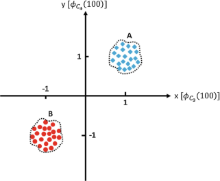
We only record from two EEG electrodes, say C3 and C4, for two conditions A and B. These two conditions are elicited when stimuli A and B are presented to our experiment subject. Each stimuli is presented 100 times, and the voltage recorded from C3 and C4 at 100 ms poststimulus is recorded in a vector, \( {\mathcal{V}}_{\phi }={\left[{\phi}_{{\mathrm{C}}_3}(100),{\phi}_{{\mathrm{C}}_4}(100)\right]}^{\mathrm{T}} \) where \( {\phi}_{{\mathrm{C}}_3}(100) \) and \( {\phi}_{{\mathrm{C}}_4}(100) \) are the recorded signals from C3 and C4 electrodes at 100 ms poststimulus, and is plotted below:
-
(i)
How could you distinguish between condition A and B if you were only given \( {\mathcal{V}}_{\phi } \)?
-
(ii)
Let us assume that \( {\mathcal{V}}_{\phi } \) under conditions A and B has the same exact distribution except that for condition A the distribution is centered around the point (1,1)T and for condition B around the point (−1,−1)T. Let us denote this probability distribution with p(x, y) and also let us assume symmetry with respect to origin, that is, p(x, y) = p(−x, −y), and indifference to input variables’ order, i.e., p(x, y) = p(y, x). Now if we want to fit the line \( y-\alpha x-\delta =0 \), such that any point lying on one side of this line is designated as condition A and the other side as condition B, how should we find (α, δ)?
-
(iii)
Based on your answer in (ii), find the optimal set of (α, δ), if any.
-
(i)
-
5.
If we assume that a dipole is placed at coordinates (x, y, z), the distance between the dipole source and field space, \( ({x}^{\prime},{y}^{\prime},{z}^{\prime}) \), is defined as \( r=\sqrt{{\left(x-{x}^{\prime}\right)}^2+{\left(y-{y}^{\prime}\right)}^2+{\left(z-{z}^{\prime}\right)}^2} \).
-
(i)
Calculate \( \nabla \left(\frac{1}{r}\right) \), where ∇ is the gradient operator defined as \( \nabla f={\left(\frac{\partial f}{\partial x},\frac{\partial f}{\partial y},\frac{\partial f}{\partial z}\right)}^{\mathrm{T}} \).
-
(ii)
Calculate \( {\nabla}^{\prime}\left(\frac{1}{r}\right) \), where ∇′ is the gradient operator with respect to \( ({x}^{\prime},{y}^{\prime},{z}^{\prime}) \), i.e., \( {\nabla}^{\prime }f={\left(\frac{\partial f}{\partial {x}^{\prime }},\frac{\partial f}{\partial {y}^{\prime }},\frac{\partial f}{\partial {z}^{\prime }}\right)}^{\mathrm{T}} \).
-
(iii)
Show that \( \nabla \left(\frac{1}{r}\right)=-{\nabla}^{\prime}\left(\frac{1}{r}\right) \).
-
(i)
-
6.
Assuming that a current dipole is placed at the origin of an infinitely homogeneous space pointing toward the z-direction, i.e., (x, y, z)T = (0, 0, 0)T and \( \overline{{\mathcal{J}}^{i}} \) = (0, 0, 1)T, using Eq. 13.3:
-
(a)
Can you calculate the potential field generated by this dipole in any point \( ({x}^{\prime},{y}^{\prime},{z}^{\prime}) \)?
Hint. \( \underset{v}{\int}\nabla \left(\frac{1}{r}\right).\overline{{\mathcal{J}}^{{i}}}\left(x,y,z\right)\ dv=\nabla \left(\frac{1}{r}\right).\overline{{\mathcal{J}}^{{i}}} \), where \( \overline{{\mathcal{J}}^{{i}}} \) is the current dipole moment at the origin and \( \nabla \left(\frac{1}{r}\right).\overline{{\mathcal{J}}^{{i}}} \) is the inner product of the dipole moment and the gradient of the reciprocal of field point distance to dipole. This equality is due to the fact that we assumed the dipole source to be a point source at the origin. This basically is the impulse response of the Poisson’s equations, more generally referred to as the Green’s function. The inner product between vectors A = (A x, A y, A z)T and B = (B x, B y, B z)T is defined as follows: A. B = A xB x + A yB y + A zB z.
-
(b)
Assuming that the EEG sensor is located at (0, 0, 1)T, what number would it read as the potential (ideal conditions, noise is nonexistent)?
-
(c)
What if the sensor is located at (1, 0, 0)T?
-
(d)
What if the sensor is located at (0, − 1, 0)T?
-
(a)
-
7.
Repeat problem 6 to calculate the magnetic field an MEG magnetometer would sense at the same locations. Use (\( B=\frac{\mu }{4\pi}\int \overline{{\mathcal{J}}^{i}}\times \nabla \left(\frac{1}{r}\right) dv \)) and the Green’s function hint given before. The cross product between vectors A = (A x, A y, A z)T and B = (B x, B y, B z)T is defined as follows: A × B = (A yB z − A zB y, A zB x − A xB z, A xB y − A yB x).
-
8.
Based on problems 6 and 7, can you explain [and prove mathematically] why EEG signals are less sensitive to tangential sources and MEG signals to radial sources?
-
9.
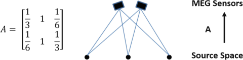
Let us simply assume that the lead field matrix A, of an MEG recording system with two recording channels and 3 possible sources, is given as follows:
-
(i)
Assuming that the given lead field matrix models the relationship between source current density and the magnetic field in z-direction, what is the relationship between the recorded magnetic field (in z-direction) B at these sensors and the current density S = (S 1,S 2,S 3)T? Assume ideal conditions where no noise exists.
-
(ii)
What would the MEG sensors record if S = (1,1,1)T?
-
(iii)
What if S = (2,−1,2)T?
-
(iv)
What if S = (3,0,3)T?
-
(v)
What if S = (1,1,1)T + \( \mathcal{t} \)(2,−1,2)T, \( \left(\mathcal{t}\in \mathcal{R}\right) \)?
-
(vi)
Can you calculate the null space of matrix A, that is, all vectors x such that Ax = 0?
-
(vii)
Can you briefly explain why the inverse problem is not unique? You can mathematically prove this using the concept of null space of a matrix.
-
(i)
-
10.
-
(i)
Can you formulate the relationship between estimated, X, and true source, S?
-
(ii)
Based on the relation derived in (i), what should be the relationship between A and B, for the estimated source to be exactly the same as the true source?
-
(iii)
Can linear methods, as studied in this problem, ever truly estimate the true source without any further priors or assumptions?
-
(i)
-
11.
Can you derive Eq. 13.16 from Eq. 13.15 by differentiating Eq. 13.15 and setting it to zero?
-
12.
Let us study the Bayesian approaches in more detail (Eqs. 13.20, 13.21, and 13.22). Let us assume that \( \phi = Ax+{n} \) and that \( {n} \) is a white Gaussian noise, \( {n}\sim N\left(0,{\sigma_n}^2\right): \)
-
(a)
What is the probability distribution function (pdf) of \( {n} \)?
-
(b)
What does p(ϕ| x) mean? Convince yourself that \( p\left(\phi |x\right)=p(n)\propto {e}^{-\frac{1}{2{\sigma_n}^2}{\left\Vert \phi - Ax\right\Vert}^2} \).
-
(c)
If we assume x ∼ N(0, σ s 2), what is p(x)?
-
(d)
Using Bayes’ rule (Eq. 13.20), formulate the posterior distribution p(x| ϕ).
-
(e)
Define the likelihood of a distribution as \( \mathcal{L}(x)=\ln p(x) \). Derive the posterior likelihood calculated in (iv).
-
(f)
Formulate \( \hat{x}=\underset{x}{\mathrm{argmax}}\mathcal{L}\left(x|\phi \right) \) and derive a similar formula to Eq. 13.15, showing that weighted minimum-norm (WMN) solutions are a form of maximum a posteriori (MAP) estimators.
-
(a)
-
13.
The L2-norm of a 2D vector, (x, y), is defined as \( \sqrt{x^2+{y}^2}, \) and the L1-norm is defined as ∣x ∣ + ∣ y∣. The level sets of norm functions are closed curves partitioning the space to inside and outside. On the other hand, some functions, such as lines or hyperplanes, partition the space to above and below. We will explore the level sets of these functions in simple cases and in a two-dimensional space. We will examine how these simple functions can be combined to form optimization problems, in later questions.
-
(a)
Can you plot \( \sqrt{x^2+{y}^2}=1 \) and |x| + |y| = 1?
-
(b)
Can you plot and describe the set of lines described by y + 2x = K 0 for \( {K}_0\in \mathcal{R} \)? If K 0 decreases, which direction will the line move toward? What happens when K 0 increases?
-
(a)
-
14.
Assuming x, y ≥ 0, how would you describe the following optimization problem?
-
(a)
\( \underset{x,y}{\mathrm{argmin}\ }\left(y+2x\right) \)
Subject to |x| + |y| = 1 x, y ≥ 0
Hint. Basically, you want to minimize K 0 (where y + 2x = K 0) for nonnegative x, y with L1-norm of 1.
-
(b)
Can you graphically depict this optimization problem, by varying the values of K 0?
-
(c)
Based on (b), can you propose a systematic way to solve this type of an optimization problem? What are the optimal values of x ∗, y ∗, and K 0 ∗ in this problem?
-
(a)
-
15.
Repeat problem 6 for the following optimization problem:
$$ \underset{x,y}{\mathrm{argmin}\ }\left(y+2x\right) $$Subject to \( \sqrt{x^2+{y}^2}=1\ x,y\ge 0 \)
-
16.
From problems 14 and 15, can you explain why you would expect L1-norm regularizations to induce sparsity in the solution? Sparsity in case of a 2D signal means only 1 nonzero element!


Rights and permissions
Copyright information
© 2020 Springer Nature Switzerland AG
About this chapter

Cite this chapter
He, B., Ding, L., Sohrabpour, A. (2020). Electrophysiological Mapping and Source Imaging. In: He, B. (eds) Neural Engineering. Springer, Cham. https://doi.org/10.1007/978-3-030-43395-6_13
Download citation
DOI: https://doi.org/10.1007/978-3-030-43395-6_13
Published:
Publisher Name: Springer, Cham
Print ISBN: 978-3-030-43394-9
Online ISBN: 978-3-030-43395-6
eBook Packages: Biomedical and Life SciencesBiomedical and Life Sciences (R0)