SOBOLHDMR: A General-Purpose Modeling Software

Abstract

One of the dominant approaches in synthetic biology is the development and implementation of minimal circuits that generate reproducible and controllable system behavior. However, most biological systems are highly complicated and the design of sustainable minimal circuits can be challenging. SobolHDMR is a general-purpose metamodeling software that can be used to reduce the complexity of mathematical models, such as those for metabolic networks and other biological pathways, yielding simpler descriptions that retain the features of the original model. These descriptions can be used as the basis for the design of minimal circuits or artificial networks.

Appendices

Appendix 1: Fast Equivalent Operational Model

Problem Statement

Consider a system of ordinary differential equations (ODE) with uncertain parameters:

$$\begin{array}{lll}{\frac{{d\mathbf{ y}}}{dt }}=F(\mathbf{ y,p},t) \\{\mathbf{ y}(t=0)}=\mathbf{ y}0(\mathbf{ p}) \end{array}$$

(1.1)

Here p is the vector of uncertain static parameters.

The objective is to approximate $\mathbf{ y}(t_i^{*},\mathbf{ p}),\;i=1,\ldots,n$ at specific time $t_i^{*}$ points with Quasi Random Sampling-High Dimensional Model Representation (QRS-HDMR) models. The original model can be expensive to run while the set of QRS-HDMR models also known as Fast Equivalent Operational Model (FEOM) can be run in milliseconds.

Solution Procedure

Sample N points of the vector $\{{{\mathbf{ p}}_j}\},\;j=1,\ldots,N$ (we recall that vector p is an input of the HDMR model), for all ${{\mathbf{ p}}_j}$ solve ODE Eq. 1.1 and obtain $K\times N$ outputs $\mathbf{ y}(t_k^{*},{{\mathbf{ p}}_j}),k=1,\ldots,K,\;j=1,\ldots,N$. Using these data as the input–output samples, build a set of the HDMR models (FEOM).

Test case:

Consider an ODE:

$$ \frac{df }{dt } = {{a^{\prime}_t}}{\sin^2}{X_2}+{{b^{\prime}_t}}\ X_3^4\sin {X_1} $$

(1.2)

with initial conditions given by the Ishigami function:

$$ {f_{t=0 }}=\sin {X_1}+{a_{t=0 }}{\sin^2}{X_2}+{b_{t=0 }}X_3^4\sin {X_1} $$

where

$$ {a_t}=7\exp \left( {-t} \right),\quad {b_t}=0.1\exp (t) $$

$$ \frac{{d{a_t}}}{dt } = {{a^{\prime}_t}},\quad \frac{{d{b_t}}}{dt }={{b^{\prime}_t}} $$

Here ${X_1},\ {X_2},\ {X_3}$ are random variable with a probability distribution function given by:

$$ {p_i}\left( {{X_i}} \right)=\left\{ {\eqalign{{\frac{1}{{2\pi }},} {\ \mathrm{ \ if}\ - \pi \leq {X_i}\leq \pi } \\{0,} \ \ \ {\mathrm{ if}\ {X_{i<- \pi, {X_i>}}}\ \pi } \\}} \right.,\quad \mathrm{ for}\ i=1,2,3 $$

The explicit solution to the above ODE is:

$$ {f_t}=\sin {X_1}+{a_t}{\sin^2}{X_2}+{b_t}X_3^4\sin {X_1} $$

At each moment of time the total variance and partial variances can be calculated explicitly [22]:

$$ \begin{array}{lll} D=\frac{{a_t^2}}{8}+\frac{{{b_t}{\pi^4}}}{5}+\frac{{b_t^2{\pi^8}}}{18 }+\frac{1}{2} \\{D_1}=\frac{{{b_t}{\pi^4}}}{5}+\frac{{b_t^2{\pi^8}}}{50 }+\frac{1}{2} \\{D_2} = \frac{{a_t^2}}{8} \\{D_3}=0 \\{D_{12 }}=0 \\{D_{13 }}=\frac{{b_t^2{\pi^8}}}{18 }-\frac{{b_t^2{\pi^8}}}{50 } \\{D_{23 }}=0 \\{D_{123 }}=0\end{array} $$

For each time-step $t=0.0,\ 0.1,\ 0.2,\ldots$ the ODE Eq. 1.2 is solved and a HDMR model is built using the corresponding output. FEOM can then be compiled by combining HDMRs for all time-steps.

Steps:

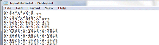
• 1. Generate N Sobol (or random for the MC method) points for the input variables ${X_1},{X_2},{X_3}$ and store in the file “IO/InputData.txt” (subdirectory “IO”). Its content looks like this (for the QMC method):

• 2. For the time-step $t=0.0$ solve ODE Eq. 1.2 for each of N random or Sobol points to obtain the corresponding output. Store the output in the file “IO/OutputData1.txt.” The fourth line in this output file should contain the value of the time-step that was used.

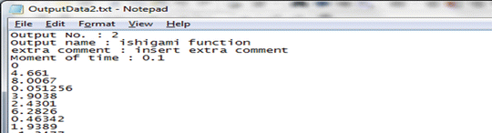
• 3. For the time-step $t=0.1$ solve ODE Eq. 1.2 for each of the N random or Sobol points to obtain the corresponding output. Store the output in the directory “IO/OutputData2.txt.” The fourth line in this output file should contain the value of the time-step that was used.

• 4. Repeat Step 3 for $t=0.2,\ 0.3,\ldots$, and store outputs files “IO/OutputData3.txt,” “IO/OutputData4.txt,” etc. Note that the fourth line in each output file should contain the contain the value of the corresponding time-step.

Running SobolHDMR with options “Function to call = tabulated_data” and “Number of outputs = 11” (currently there are 11 output files in the “IO” folder) will create the FEOM for the above ODE example with $t=0.0,\ 0.1,\ldots,1.0$

The same GUI page that is used to view sensitivity results produces the following plots (Fig. 19):

Fig. 19

(a) First-order sensitivity indices versus time for Input 1; (b) total-order sensitivity indices versus time for Input 1

Figure 20 presents the FEOM using the first three input points from the file “IO/InputData.txt”

Fig. 20

HDMR output as a function of time (for the first three input data points)

Appendix 2: Theoretical Background

The deletion of high order members arises from a metamodeling context. Quite often in mathematical models, only relatively low order interactions of input variables have the main impact on the model output. For such models, the computation of the sensitivity terms of Eq. 2.29 is best carried out by the RS‐HDMR technique as proposed by Li et al., which, as a metamodeling technique, has the more general utility of providing a representation of the input–output mapping over the whole input space [5].

Metamodels, also known as surrogate models, are resorted to when the underlying mathematical structure of a model is complex and contains many input variables. These approximate models are cheaper to evaluate than the original functions that they mimic. For black-box models or laboratory observations where mechanistic models do not exist, metamodels help provide a better understanding of the underlying relationship between inputs and outputs.

The underlying framework of all metamodeling techniques consists of a data collection strategy, the selection of a model type, and the fitting of the model to the data [17]. The fitting of the model is usually done by finding optimal values of certain model parameters that minimize an approximation-error function; such methods include least squares, best linear predictor, log-likelihood, and so on.

There are a variety of model types for approximating complex, multivariate functions. Response surface methodologies usually approximate the complex multivariate function by low order polynomials, such as

$$ \tilde{Y}={\beta_o}+\sum\limits_{i=1}^k {{\beta_i}{X_i}} +\sum\limits_{i=1}^k {{\beta_{ii }}X_i^2} +\sum\limits_{i=1}^{k-1 } {\sum\limits_{j>i}^k {{\beta_{ij }}{X_i}{X_j}} } $$

(1.3)

where $\tilde{Y}$ is an approximation to Eq. 2.5 with the parameters β _o , β _i , … being determined by some form of least square regression [18]. Kriging is an interpolative approximation method based on the weighted sum of the sampled data. It is a combination of a polynomial model plus departures which are realization of a random function [2]. Neural networks have been used to approximate a multivariate function as a nonlinear transformation of multiple linear regression models [18]. Although these techniques are useful for particular applications, they fall short in certain areas. Response surface methodologies are not accurate enough to approximate complex nonlinear multimodal profiles as they are based on simple quadratic models. Kriging models are difficult to obtain or even use [17]. Training of neural networks usually takes a lot of computing time [18]. A promising metamodeling tool for approximating complex, multivariate functions is the HDMR.

High Dimensional Model Representation

HDMR can be regarded as a tool for capturing high dimensional input–output system behavior. It rests on the generic assumption of only low order input correlations playing a significant role in physical systems. The HDMR expansions can be written in the following form for $f(x)\equiv f({x_1},\ {x_2},\ldots,{x_n})$ as

$$\begin{array}{lll} f(x)={f_o}+\mathop{\sum}\limits_i{f_i}\left( {{x_i}} \right)+\mathop{\sum}\limits_i\mathop{\sum}\limits_{j>i }{f_{ij }}\left( {{x_i},{x_j}} \right)+\cdots\cr\quad +{f_{{12\ldots k}}}\left( {{x_1},\ldots,{x_n}} \right) \end{array}$$

(1.4)

This decomposition is unique, called an ANOVA-HDMR decomposition, if the mean of each term with respect to its variable is zero as given in Eq. 2.25, resulting in pairs of terms being orthogonal [4]. Each term of the ANOVA-HDMR decomposition tells of the contribution of the corresponding group of input variables to the model output f(x). The determination of all the terms of the ANOVA-HDMR requires the evaluation of high dimensional integrals, which would be carried out by Monte Carlo integration. For high accuracy, a large number of sample points would be needed. This represents a serious drawback of the ANOVA-HDMR. For most practical applications, rarely are terms beyond three-order significant [4]. Rabitz and coworkers proposed a Random Sampling-HDMR (RS-HDMR) which involves truncating the HDMR expansions up to the second or third order, and then approximating the truncated terms by orthonormal polynomials [5, 19].

Consider a piecewise smooth and continuous component function. It can be expressed using a complete basis set of orthonormal polynomials:

$$ {f_i}\left( {{x_i}} \right)=\mathop{\sum}\limits_{r=1}^{\infty}\alpha_r^i{\varphi_r}\left( {{x_i}} \right) $$

(1.5)

$$ {f_{ij }}\left( {{x_i},{x_j}} \right)=\mathop{\sum}\limits_{p=1}^{\infty}\mathop{\sum}\limits_{q=1}^{\infty}\beta_{pq}^{ij }{\varphi_{pq }}\left( {{x_i},{x_j}} \right) $$

(1.6)

$$ \ldots $$

Here ${\varphi_r}\left( {{x_i}} \right),\;\ {\varphi_{pq }}\left( {{x_i},{x_j}} \right)$ are sets of one- and two-dimensional basis functions (Legendre polynomials) and $\alpha_r^i$ and $\beta_{pq}^{ij }$ are coefficients of decomposition which can be determined using orthogonality of the basis function:

$$ \alpha_r^i=\int\nolimits_0^1 {{f_i}\left( {{x_i}} \right){\varphi_r}\left( {{x_i}} \right)d{x_i}}, \quad r=1,\ldots,k $$

(1.7)

$$ \beta_{pq}^{ij }=\int\nolimits_0^1 {\int\nolimits_0^1 {{f_i}\left( {{x_i}} \right){\varphi_p}\left( {{x_i}} \right){\varphi_q}({x_j})d{x_i}d{x_j}} } $$

$$ p=1,\ldots,l,\quad q=1,\ldots,{l}^{\prime} $$

(1.8)

In practice the summation in Eqs. 5 and 6 is limited to some maximum orders k, l, l′:

$$ {f_i}\left( {{x_i}} \right)\approx \mathop{\sum}\limits_{r=1}^k\alpha_r^i{\varphi_r}\left( {{x_i}} \right) $$

(1.9)

$$ {f_{ij }}\left( {{x_i},{x_j}} \right)\approx \mathop{\sum}\limits_{p=1}^l\mathop{\sum}\limits_{q=1}^{{l^{\prime}}}\beta_{pq}^{ij }{\varphi_{pq }}\left( {{x_i},{x_j}} \right) $$

(1.10)

The first few Legendre polynomials are:

$$ {\varphi_1}(x) = \sqrt{3}\left( {2x-1} \right) $$

$$ {\varphi_2}(x)=6\ \sqrt{5}\left( {{x^2}-x+\frac{1}{6}} \right) $$

(1.11)

$$ {\varphi_3}(x) = 20\ \sqrt{7}\left( {{x^3}-\frac{3}{2}{x^2}+\frac{3}{5}x-\frac{1}{20 }} \right) $$

$$ \ldots $$

Coefficients of the decomposition and are related to the first-, second-, and third-order sensitivity indices by [6, 8]:

$$ {S_i}\approx \frac{{\mathop{\sum}\nolimits_{r=1}^k{{{\left( {\alpha_r^i} \right)}}^2}}}{V} $$

$$ {S_{ij }}\approx \frac{{\mathop{\sum}\nolimits_{p=1}^l\mathop{\sum}\nolimits_{q=1}^{{l^{\prime}}}{{{\left( {\beta_{pq}^{ij }} \right)}}^2}}}{V} $$

$$ {S_{ijk }}\approx \frac{{\mathop{\sum}\nolimits_{p=1}^m\mathop{\sum}\nolimits_{q=1}^{{m^{\prime}}}\mathop{\sum}\nolimits_{r=1}^{{m^{\prime\prime}}}{{{\left( {\gamma_{pqr}^{ijk }} \right)}}^2}}}{V} $$

where V, the total variance, is given by Eq. 2.28. The optimal values of $\alpha_r^i$, $\beta_{pq}^{ij }$, and $\gamma_{pqr}^{ijk }$, determined by a least squares minimization criteria, are given by [5].

Typically, the higher the number of component functions in the truncated expansion, the higher will be the number of sampled points N needed to evaluate the polynomial coefficients with sufficient accuracy. Li and Rabitz proposed the use of ratio control variate methods to improve the accuracy of Eq. 2.35 in estimating $\alpha_r^i$, $\beta_{pq}^{ij }$, and $\gamma_{pqr}^{ijk }$ [14]. Feil et al. used quasi-random points instead of pseudorandom numbers for improving the accuracy of Eq. 2.35; they proposed determining an optimal number of points N _opt, such that the variance in $\alpha_r^i$ as a function of N in two consecutive simulations was within some tolerance [3].

Integers κ, l, l′, m, m′, and m″ in Eq. 2.33 are the polynomial orders, and an important problem is the choice of the optimal values for these integers. Ziehn and Tomlin proposed using a least squares minimization technique in determining the optimal polynomial order between [0, 3] for each component function [20]. Feil et al. proposed the use of the convergence of the sensitivity indices of Eq. 2.34 in defining optimal polynomial orders for each component function [3].

For a model with a high number of input parameters and significant parameter interactions, Ziehn and Tomlin recommend first applying a screening method such as the Morris method to reduce the dimensionality of the problem and thus improve the accuracy of the estimation of high order component functions for smaller sample sizes [20].

The error of the model approximation can be measured, similarly to Eq. 2.30, by the scaled distance:

$$ \delta \left( {f,\tilde{f}} \right)=\frac{1}{V}\int {{{{\left[ {f(x)-\tilde{f}(x)} \right]}}^2}dx} $$

(1.12)

where $f(x)$ is the original function and $\tilde{f}(x)$ the approximation. This scaling serves as a benchmark to distinguish between good and bad approximation; for if the mean ${f_o}$ is used as the approximant, that is, if $\tilde{f}(x)={f_o}$, then $\delta =1$. Thus a good approximation is one with $\delta \ll 1$ [19, 21].

Metamodels play an important role in the analysis of complex systems. They serve as an effective way of mapping input–output relationships and of assessing the impact of the inputs on outputs. Metamodels can also be applied to solve various types of optimization problems that involve computation-intensive functions.

One of the very important and promising developments of model analysis is the replacement of complex models and models which need to be run repeatedly online with equivalent “operational metamodels.”

There are a number of techniques for approximating complex, multivariate functions. Response surface methodologies usually approximate the complex multivariate function by low order polynomials, such as

$$ \tilde{Y}={\beta_o}+\sum\limits_{i=1}^k {{\beta_i}{X_i}} +\sum\limits_{i=1}^k {{\beta_{ii }}X_i^2} +\sum\limits_{i=1}^{k-1 } {\sum\limits_{j>i}^k {{\beta_{ij }}{X_i}{X_j}} } $$

(1.13)

where $\tilde{Y}$ is an approximation to Eq. 2.5 with the parameters β _o , β _i , … being determined by some form of least square regression [18]. Kriging is an interpolative approximation method based on the weighted sum of the sampled data. It is a combination of a polynomial model plus departures which are realization of a random function [2]. Neural networks have been used to approximate a multivariate function as a nonlinear transformation of multiple linear regression models [18]. Although these techniques are useful for particular applications, they fall short in certain areas. Response surface methodologies are not accurate enough to approximate complex nonlinear multimodal profiles as they are based on simple quadratic models. Kriging models are difficult to obtain or even use [17]. Training of neural networks usually takes a lot of computing time [18]. A promising metamodeling tool for approximating complex, multivariate functions is the HDMR.

One major problem associated with traditionally used parameterized polynomial expansions and interpolative look-up tables is that the sampling efforts grow exponentially with respect to the number of input variables. For many practical problems only low order correlations of the input variables are important. By exploiting this feature, one can dramatically reduce the computational time for modeling such systems. An efficient set of techniques called HDMR was developed by Rabitz and coauthors [6, 14]. A practical form of HDMR, Random Sampling-HDMR (RS-HDMR), has recently become a popular tool for building metamodels [20]. Unlike other input–output mapping methods, HDMR renders the original exponential difficulty to a problem of only polynomial complexity and it can also be used to construct a computational model directly from data.

Variance-based methods are one of the most efficient and popular global SA techniques. However, these methods generally require a large number of function evaluations to achieve reasonable convergence and can become impractical for large engineering problems. RS-HDMR can also be used for GSA. This approach to GSA is considerably cheaper than the traditional variance-based methods in terms of computational time as the number of required function evaluations does not depend on the problem dimensionality. However, it can only provide estimates of the main effects and low order interactions.

ANOVA: High Dimensional Model Representation

Recall, that an integrable function $f\left( \boldsymbol{ x} \right)$ defined in the unit hypercube ${H^n}$ can be expanded in the following form:

$$ f\left( \boldsymbol{ x} \right)={f_o}+\mathop{\sum}\limits_{i=1}^n\mathop{\sum}\limits_{{{i_{{1<\ldots< }}}{i_s}}}^s{f_{{{i_1}\ldots {i_s}}}}({x_{{{i_1}}}},\ldots,\ {x_{{{i_s}}}}) $$

This expansion is unique if

$$ \int\nolimits_0^1 {{f_{{{i_1}\ldots {i_s}}}}({x_{{{i_1}}}},\ldots,{x_{{{i_s}}}})d{x_{{{i_k}}}}=0}, \quad 1\leq k\leq s $$

(1.14)

in which case it is known as the ANOVA-HDMR decomposition. It follows from condition that the ANOVA-HDMR decomposition is orthogonal.

Rabitz argued (in [6]) that for many practical problems only the low order terms in the ANOVA-HDMR decomposition are important and $f\left( \boldsymbol{ x} \right)$ can be approximated by

$$ \hat{f}\left( \boldsymbol{ x} \right)={f_o}+\sum\limits_{i=1}^d {\sum\limits_{{{i_{{1<\ldots <}}}{i_s}}}^s {{f_{{{i_{{1\ldots }}}{i_s}}}}({x_{{{i_1}}}},\ldots,{X_{{{i_s}}}})} } $$

Here d is a truncation order, which for many practical problems can be equal to 2 or 3.

Approximation of ANOVA-HDMR Component Functions

The RS-HDMR method proposed in Li and Rabitz and Li et al. aims to reduce the sampling effort by approximating the component functions by expansions in terms of a suitable set of functions, such as orthonormal polynomials [6, 14].

Consider piecewise smooth and continuous component functions. Using a complete basis set of orthonormal polynomials they can be expressed via the expansion:

$$ {f_i}\left( {{x_i}} \right)=\mathop{\sum}\limits_{r=1}^{\infty}\alpha_r^i{\varphi_r}\left( {{x_i}} \right) $$

$$ {f_{ij }}\left( {{x_i},{x_j}} \right)=\mathop{\sum}\limits_{p=1}^{\infty}\mathop{\sum}\limits_{q=1}^{\infty}\beta_{pq}^{ij }{\varphi_{pq }}\left( {{x_i},{x_j}} \right) $$

Here ${\varphi_r}\left( {{x_i}} \right),\;{\varphi_{pq }}\left( {{x_i},{x_j}} \right)$ are sets of one- and two-dimensional basis functions and $\alpha_r^i,\;\beta_{pq}^{ij }$ are coefficients of decomposition which can be determined using orthogonality of the basis functions:

$$ \alpha_r^i=\int\nolimits_0^1 {{f_i}\left( {{x_i}} \right){\varphi_r}\left( {{x_i}} \right)d{x_i}}, \quad r=1,\ldots,k $$

(1.15)

$$ \beta_{pq}^{ij }=\int\nolimits_0^1 {\int\nolimits_0^1 {{f_i}\left( {{x_i}} \right){\varphi_p}\left( {{x_i}} \right){\varphi_q}({x_j})d{x_i}d{x_j}} } $$

(1.16)

$$ p=1,\ldots,l,\quad q=1,\ldots,{l}^{\prime} $$

In practice the summation in Eqs. 1.15 and 1.16 is limited to some maximum orders $k,l,{l}^{\prime}$:

$$ {f_i}\left( {{x_i}} \right)\approx \mathop{\sum}\limits_{r=1}^k\alpha_r^i{\varphi_r}\left( {{x_i}} \right) $$

$$ {f_{ij }}\left( {{x_i},{x_j}} \right)\approx \mathop{\sum}\limits_{p=1}^l\mathop{\sum}\limits_{q=1}^{{l^{\prime}}}\beta_{pq}^{ij }{\varphi_{pq }}\left( {{x_i},{x_j}} \right) $$

The question of how to find maximum orders is discussed in the following sections. Shifted Legendre polynomials are orthogonal in the interval [0,1] with unit weight and they are typically used for uniformly distributed inputs. The higher dimensional polynomials can be expressed as the product of one-dimensional ones.

The first few Legendre polynomials are:

$$ {\varphi_1}(x)=\sqrt{3}\left( {2x-1} \right) $$

$$ {\varphi_2}(x)=6\sqrt{5}\left( {{x^2}-x+\frac{1}{6}} \right) $$

(1.17)

$$ {\varphi_3}(x)=20\sqrt{7}\left( {{x^3}-\frac{3}{2}{x^2}+\frac{3}{5}x-\frac{1}{20 }} \right) $$

Decomposition coefficients are usually evaluated using Monte Carlo integration, which can be inaccurate especially at small number of sampled points N. It was shown that in the approximation of higher order polynomial expansions with a small number of sampled points N, oscillations of the component functions may occur around the exact values [6]. The integration error can be reduced either by increasing the sample size N or by applying the variance reduction techniques proposed in Li and Rabitz [14]. Feil et al. suggested using QMC sampling to reduce oscillations and the integration error [3].

Evaluation of Global Sensitivity Indices Based on RS-HDMR

For a continuous function with piecewise derivatives the following relationship exists between the square of the function and the coefficients of its decomposition ${c_r}$ with respect to a complete set of orthogonal polynomials (Parseval’s theorem):

$$ \int\nolimits_0^1 {f{(x)^2}dx} =\mathop{\sum}\limits_{r=1}^{\infty }{{({c_r})}^2} $$

Application of Parseval’s theorem to the component functions of ANOVA-HDMR and definitions of SI yield the following formulas for SI:

$$ {S_i}=\frac{{\mathop{\sum}\nolimits_{r=1}^{\infty }{{{(a_r^i)}}^2}}}{D} $$

$$ {S_{ij }}=\frac{{\mathop{\sum}\nolimits_{p=1}^{\infty }{{{(\beta_{pq}^{ij })}}^2}}}{D} $$

where D is the total variance.

For practical purposes, function decompositions truncated at some maximum order of polynomials are used:

$$ {S_i}\approx \frac{{\mathop{\sum}\nolimits_{r=1}^k{{{\left( {\alpha_r^i} \right)}}^2}}}{V} $$

$$ {S_{ij }}\approx \frac{{\mathop{\sum}\nolimits_{p=1}^l\mathop{\sum}\nolimits_{q=1}^{{l^{\prime}}}{{{\left( {\beta_{pq}^{ij }} \right)}}^2}}}{V} $$

$$ {S_{ijk }}\approx \frac{{\mathop{\sum}\nolimits_{p=1}^m\mathop{\sum}\nolimits_{q=1}^{{m^{\prime}}}\mathop{\sum}\nolimits_{r=1}^{{m^{\prime\prime}}}{{{\left( {\gamma_{pqr}^{ijk }} \right)}}^2}}}{V} $$

The total number of function evaluations required for calculation of a full set of main effect and total SI using the general Sobol’ formulas is ${N_F}=N(n+2)$ [10]. To compute SI using RS-HDMR or QRS-HDMR only ${N_F}=N$ function valuations is required, which is n + 2 times less than for the original Sobol method for the same number of sampled points. However, in practice RS-HDMR or QRS-HDMR can only provide sets of first- and second-order (up to third) SI.

How to Choose the Maximum Order of Polynomials

An important problem is how to choose an optimal order of the orthogonal polynomials. In majority of published works by Rabitz and coauthors the fixed order polynomials (up to the second or third order) were used. However, in some cases polynomials up to the tenth order were used, although no explanation for the choice of such a high order polynomials were given.

This problem of optimal maximum order polynomials was considered by Ziehn and Tomlin [20]. They proposed to use an optimization method to choose the best polynomial order for each component function. They also suggested excluding any component function from the HDMR expansion which does not contribute to the HDMR expansion. The overheads for using an optimization method can be considerable. We suggest a different approach to define optimal polynomial orders based on the estimated convergence of SI calculated by RS(QRS)-HDMR.

Typically the values of decomposition coefficients, $a_r^i$, $\beta_{pq}^{ij }$, etc., rapidly decrease with increasing the order of r and (p, q). As a result the truncation error is dominated by the first few truncation coefficients.

Another important issue is how to define a sufficient number of sampling points in MC or QMC integration of the polynomial coefficients, $a_r^i$, $\beta_{pq}^{ij }$. Although in a limit

$$ \mathop{\lim}\limits_{ k\to \infty \atop N\to \infty }\sum\limits_{r=1}^k {{{{\left( {\hat{a}_r^i(N)} \right)}}^2}={S_i}} $$

(the same asymptotic rule apply for other coefficients) but practically the accuracy of coefficients approximation depends on the number of sampled points N: $\hat{a}_r^i=\hat{a}_r^i(N)$. Typically, the higher the order of the component function the higher the number of sampled points required to evaluate the polynomial coefficients with sufficient accuracy [6].

To determine an optimal number of points ${N_{\mathrm{ opt}}}$ it is sufficient to examine the variance of $a_r^i$, r = 1, 2 as a function of N. N is increased sequentially and N at which a required tolerance of the variance is reached is taken as ${N_{\mathrm{ opt}}}$.

After a sufficient number of function evaluations ${N_{\mathrm{ opt}}}$ is made, the convergence of the estimated sensitivity indices with respect to the polynomial orders is monitored. For the first-order component functions the contribution of the subsequent $a_{k+1}^i$ coefficient is analyzed by monitoring its relative or absolute (in the case of small values of ${S_i}$) contribution:

$$ \eqalign{\frac{{{{{\left( {a_{k+1}^i} \right)}}^2}}}{{\mathop{\sum}\nolimits_{r=1}^{k+1 }{{{\left( {a_r^i} \right)}}^2}}}<{\epsilon_1}\ \mathrm{ if}\ \mathop{\sum}\limits_{r=1}^{k+1 }{{\left( {a_r^i} \right)}^2}>{10^{-4 }} \\{{\left( {a_{k+1}^i} \right)}^2}<{\epsilon_1}\text{, otherwise}}$$

For the second-order component functions the procedure is more complex because it requires monitoring convergence in a two-dimensional space of p and q polynomial orders.

References

Saltelli A, Ratto M et al (2008) A new derivative based importance criterion for groups of variables and its link with the global sensitivity indices. Wiley, West Sussex
Sathyanarayanamurthy H, Chinnam RB (2009) Metamodels for variable importance decomposition with applications to probabilistic engineering design. Comput Ind Eng 57:996–1007
Kucherenko S, Fernandez MR, Pantelide C, Shah N (2009) Monte Carlo Evaluation of derivative-based global sensitivity measures. Reliab Eng Syst Saf 94:1135–1148
Rabitz H, Alis OF et al (1999) Efficient input–output model representations. Comput Phys Commun 117:11–20
Li G, Wang S, Rabitz H (2002) Practical approaches to construct RS-HDMR component functions. J Phys Chem 106:8721–8733
Li G, Wang S et al (2002) Global uncertainty assessment by high dimensional model representation (HDMR). Chem Eng Sci 57:4445–4460
Li ZQ, Xiao YG, Li ZMS (2006) Modeling of multi-junction solar cells by Crosslight APSYS. http://lib.semi.ac.cn:8080/tsh/dzzy/wsqk/SPIE/vol6339/633909.pdf. Accessed 18 June 2010
Feil B, Kucherenko S, Shah N (2009) Comparison of Monte Carlo and Quasi-Monte Carlo sampling methods in High Dimensional Model Representation. In: Proc First International Symposium Adv System Simulation, SIMUL 2009, Porto, Portugal, 20–25 September 2009
Zuniga MM, Kucherenko S, Shah N (2013) Metamodelling with independent and dependent inputs. Comput Phys Commun 184(6):1570–1580
Sobol’ IM, Tarantola S et al (2007) Estimating the approximate error when fixing unessential factors in global sensitivity analysis. Reliab Eng Syst Saf 92:957–960
Sobol IM, Kucherenko S (2009) Derivative based global sensitivity measures and their link with global sensitivity indices. Math Comput Simul 79:3009–3017
Sobol IM, Kucherenko S (2010) A new derivative based importance criterion for groups of variables and its link with the global sensitivity indices. Comput Phys Commun 181:1212–1217
Kucherenko S, Zaccheus O, Munoz ZM (2012) SobolHDMR User manual. Imperial College London, London
Li G, Rabitz H (2006) Ratio control variate method for efficiently determining high-dimensional model representations. J Comput Chem 27:1112–1118
Kucherenko S, Feil B, Shah N, Mauntz W (2011) The identification of model effective dimensions using global sensitivity analysis. Reliab Eng Syst Saf 96:440–449
Sobol’ IM (2001) Global sensitivity indices for nonlinear mathematical models and their Monte Carlo estimates. Comput Simul 55:271–280
Wang GG, Shan S (2006) Review of metamodeling techniques in support of engineering design optimization. http://74.125.155.132/scholar?q=cache:_NCLv92moGkJ:scholar.google.com/&hl=en&as_sdt=2000. Accessed 14 Jan 2010
Simpson TW, Peplinski JD, Koch PN, Allen JK (2001) Metamodels for computer-based engineering design: survey and recommendations. Eng Comput 17:129–150
Wang SW, Georgopoulos PG, Li G, Rabitz H (2003) RS-HDMR with nonuniformly distributed variables: application to integrated multimedia/multipathway exposure and dose model for trichloroethylene. J Phys Chem 107:4707–4716
Ziehn T, Tomlin AS (2008) Global sensitivity analysis of a 3D street canyon model—part I: the development of high dimensional model representations. Atmos Environ 42:1857–1873
Sobol’ IM (2003) Theorems and examples on high dimensional model representation. Reliab Eng Syst Saf 79:187–193
Homma T, Saltelli A (1996) Importance measures in global sensitivity analysis of nonlinear models. Reliab Eng Syst Safety 52:1–17
Author information
Authors and Affiliations
Editor information
Editors and Affiliations