
Abstract
Genetic analysis of sequence data is central to determining the evolutionary history and molecular epidemiology of viruses, particularly those such as influenza A virus that have complex ecosystems involving multiple hosts. Here we provide an outline of routine phylogenetic analyses of influenza A viruses including multiple sequence alignment, selecting the best-fit evolutionary model and phylogenetic tree reconstruction using Neighbor joining, Maximum likelihood, and Bayesian inference.
You have full access to this open access chapter, Download protocol PDF
1 Introduction
In recent years, much research has focused on the evolutionary history and molecular epidemiology of influenza A viruses (1). Current efforts in influenza surveillance and sequencing have resulted in phenomenal amounts of data being made publicly available. The recent emergence of the H1N1/2009 pandemic virus provided a timely example of the importance and power of phylogenetic analysis to inform both the planning and response to newly emerged viruses (2). This chapter focuses on the phylogenetic analyses of influenza A virus genomic sequence data to infer their evolutionary history. Basic strategies used to characterize these will be described: from dataset design to alignment and tree building.
The relationships of rapidly evolving RNA viruses like influenza A are best represented by phylogenetic trees (3). Phylogenetic analysis establishes the evolutionary history and relationship between genes by inferring the common history of the genes. To achieve this, homologous regions (e.g., the coding region of the hemagglutinin (HA) gene), are compared in a multiple sequence alignment. Influenza A viruses have a small segmented genome most of which is protein coding (4). This makes multiple sequence alignment easy when compared to other more diverse and sparsely sampled viruses such as coronaviruses. However, influenza A viruses undergo frequent genetic mixing, termed reassortment, and caution must be used during analyses and interpretation of the whole genomes. Inappropriate analysis and/or dataset design can lead to inaccurate results and erroneous interpretations of the molecular epidemiology of influenza A viruses.
Three tree building methods; Neighbor joining (NJ), Maximum likelihood (ML), and Bayesian inference (BI) are described here. These methods are all statistically consistent; however, they are presented in order of increasing statistical robustness and computational cost. These methods require an explicit evolutionary model as accurate and realistic substitution models allow for greater robustness. A model testing and selection tool is also described. While the methods and examples provided here are specific for influenza A viruses, the platforms, programs, and methods are easily portable to other virus families.
2 Materials
These instructions were written with Mac OS X in mind, but should also be applicable to other operating systems. A list of databases and programs and from where they can be obtained is provided below—where possible we have used freely available programs.
2.1 Dataset Design
-
1.
NCBI GenBank Influenza Virus Resource at NCBI—http://www.ncbi.nlm.nih.gov/genomes/FLU/FLU.html (5) (see Note 1).
2.2 Multiple Sequence Alignment
-
1.
Multiple sequence alignment based on fast Fourier transform (MAFFT). Available as a standalone program (Linux/UNIX, Mac OS X, Windows) or online—http://align.bmr.kyushu-u.ac.jp/mafft/software/ (6, 7).
-
2.
Se-Al (Mac OS X)—http://tree.bio.ed.ac.uk/software/seal/ (see Note 2).
2.3 Selecting the Best-Fit Evolutionary Model
-
1.
jModelTest: phylogenetic model averaging (JAVA program that will run on Linux, Mac OS X, and Windows)—http://darwin.uvigo.es/software/jmodeltest.html (8).
2.4 Phylogenetic Reconstruction
-
1.
Neighbor joining (NJ). PAUP*: Phylogenetic Analysis Using Parsimony (and Other Methods) (Mac OS X, UNIX, Windows, or DOS-based formats)—http://paup.csit.fsu.edu/ (9).
-
2.
Maximum likelihood (ML). GARLI: Genetic Algorithm for Rapid Likelihood Inference (Linux/UNIX, Mac OS X, and Windows) http://garli.nescent.org (10).
-
3.
Bayesian inference (BI). MrBayes: Bayesian Inference of Phylogeny (Linux/UNIX, Mac OS X, and Windows)—http://mrbayes.csit.fsu.edu/ (11).
-
4.
Viewing and manipulating trees. Figtree (Linux/UNIX, Mac OS X, and Windows)—http://tree.bio.ed.ac.uk/software/figtree/.
3 Methods
3.1 Data Formats and Dataset Design
3.1.1 FASTA and NEXUS Formats
Numerous data formats are used in phylogenetic analysis, but the most common are FASTA (or Pearson) and NEXUS. FASTA is a text-based format for representing nucleotide or amino acid sequences that is easy to manipulate and process using simple text programs. A sequence in FASTA format consists of a single-line description that starts with a “>” (greater-than) followed by lines of sequence data. The description line most commonly contains the virus name. When a sequence is downloaded from public sequence databases as FASTA format, the description line most often includes additional information associated with the sequence (i.e., accession number, gene information, or collection information). The sequence data that follows the description line may be of multiple lines, for example:

NEXUS format has been extensively used in sequence analysis and is accepted by many different software packages (12). NEXUS format is composed of a number of separate blocks and standardized commands. These blocks can either be public or private blocks. Public blocks are utilized by multiple programs and house information about taxa (which in this case are viruses), morphological and molecular characters, genetic distances, genetic codes, assumptions, datasets, or phylogenetic trees. In contrast, private blocks contain information relevant to single programs such as PAUP*, GARLI, or MrBayes. The format is naturally extensible and flexible, and can be created from scratch using a text editor or exported from other software that creates NEXUS formatted files (e.g., Se-Al: File>Export>File Format).
The first line in a NEXUS format file is “#NEXUS”. This tells the software program that the file is in NEXUS format and will contain information in blocks that start with “begin” and end with “end”—with each remark separated by a semi-colon (;). Small variations exist in how different computer programs read the NEXUS format and these are most often associated with the treatment of special characters in taxa names. For example, “/” is unrecognized by PAUP* unless defined in the DATA block. In order to resolve these commonly encountered issues taxa names are often read enclosed in single quotation marks (i.e., ‘A/mallard/Alberta/300/1977(H4N3)’). However, single quotes are not recognized by MrBayes. Comments can be included in the NEXUS file but must be enclosed within square brackets “[ ]”, which informs the program to ignore the enclosed text. An example of NEXUS format is as follows:

A great advantage of a NEXUS file is that a block of instructions can be placed at the end of the file that can instruct programs, such as PAUP*, when conducting analyses. This will be addressed in Subheading 3.4.
3.1.2 Influenza Specific Dataset Preparation Criteria
-
1.
It is critical that reference sequences, obtained from public databases, are included in an analysis of virus sequences generated through sampling from surveillance studies or an outbreak. This provides a framework to understand the diversity of any newly generated sequence data in relation to previous work.
-
2.
While it is always good to start from the largest possible dataset (i.e., all available sequences in public databases), this is usually not feasible due to computational limitations, or in some cases it may not be necessary. In general the criteria below can be used during taxon sampling.
-
3.
BLAST search results: Initial dataset size can be reduced using tools such as a BLAST search. BLAST identifies sequences from a database (usually GenBank) that have the highest percentage similarity to the query sequence. It is important to note that the results of a BLAST search may not represent the closest related sequences in terms of phylogenetic relationships. Only a phylogenetic analysis will provide information on the relatedness of gene sequences. Furthermore, the results of a BLAST search are listed by highest similarity and earliest released sequence—if there are 10 BLAST hits with identical percentage similarity, these results will be listed from oldest to newest. Merely choosing the top BLAST hits is therefore not a suitable method for designing a dataset.
-
4.
Gene segment: When analyzing surface protein genes (HA or neuraminidase, NA) it is essential that you include only the subtype that is under study, or generate individual datasets for each subtype under study. However, in the case of internal gene segments (PB2, PB1, PA, NP, M, and NS), all subtypes of influenza A virus sequences can be aligned together. This is particularly important if one wishes to detect reassortment of gene segments between viruses of different subtypes.
3.2 Multiple Sequence Alignment
Multiple sequence alignments form the basis for all subsequent analyses, such as evolutionary model selection and tree building. Influenza A viruses have a small genome consisting of primarily protein-coding regions, therefore alignment is fairly simple. But incorrect alignments (especially for datasets with greater genetic diversity) may lead to dramatically misleading results; therefore, extreme caution should be taken to maximize the correctness of the alignment (see Note 3).
3.2.1 Multiple Sequence Alignment Using MAFFT
-
1.
For downloading, installation, and basic usage instructions please see the MAFFT Web site (see Note 4).
-
2.
MAFFT contains many modes of alignments where speed and accuracy are inversely proportional—from fast and inaccurate to slow and accurate.
-
3.
MAFFT provides command aliases for all of these fast and slow methods.
-
4.
Run MAFFT through the Terminal window (Finder > Applications > Utilities > Terminal).
-
5.
cd to your working folder and type “mafft” to start the program (see Fig. 1). You will be first asked to specify the input file (i.e., H5_align.fas) and then the output file (e.g., H5_align_out.fas). You will then be asked to specify a number of alignment criteria. For influenza genes we can use the defaults, which specifies the FFT-NS-2 (Fast but rough) strategy (see Note 3).
Fig. 1. 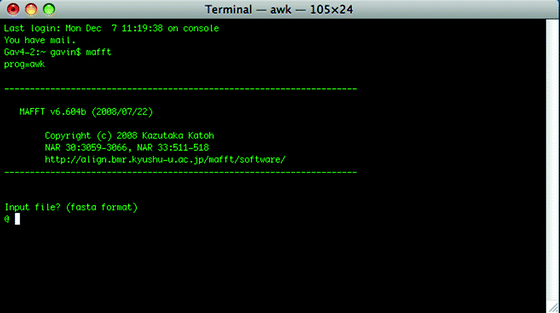
The MAFFT terminal window.
-
6.
Upon completion, the aligned sequence is stored within the output file. Manual inspection and optimization is necessary for most alignments as no alignment program is perfect.

3.2.2 Optimization of Multiple Sequence Alignment Using Se-Al
-
1.
Double-click the Se-Al icon (Finder > Applications > Utilities > Terminal) to open the program. From the Se-Al menu select “File > Open” and select the MAFFT output file (i.e., H5_align_out.fas).
-
2.
The main areas of the alignment that are likely to need manual optimization are the start and end of the alignment where not all sequences in public databases are incomplete at the 5′ and 3′ terminals. Other areas that may be misaligned include the connecting peptide of the HA, and the NA stalk that may have a deletion. However, it is important that the entire alignment be visually inspected and any misalignments corrected.
-
3.
For nucleotide sequences of protein-coding genes there are three visualization modes: nucleotides: edit an alignment of single bases; codons: edit an alignment of codons in any reading frame; and translation: edit an alignment of inferred amino acids translated using various genetic codes (influenza A virus genes utilize the universal genetic code) (see Note 5).
-
4.
Alignments can be edited by selecting a block of sequences and sliding the block relative to the other sequences wherein gaps will open up behind the block. In addition, sequences and their labels can be edited in a separate window by double-clicking on the virus name.
-
5.
In order to ease visualization of the aligned file use block colors (select “Alignment > Use Block colors”). This is especially useful when optimizing codon alignments, as amino acids are colored based on size and polarity.
-
6.
Shifting reading frames, reversing, and complementation can be done independently to any sequence or to the whole alignment and can be reversed.
-
7.
Alignments from Se-Al can be exported in numerous formats, including FASTA and NEXUS. From the menu select “File > Export” and a new dialogue window will open where the export format can be selected (see Note 6).
3.3 Selecting an Evolutionary Model
jModelTest uses hierarchical likelihood ratio tests (hLRTs) and the Akaike Information Criterion (AIC) to find the evolutionary model that best fits the particular sequence alignment that you are analyzing (8) (see Note 7). If you modify your dataset you should recalculate the evolutionary model.
-
1.
Double-click the jModelTest.jar file to open the program console as shown in Fig. 2.
Fig. 2. 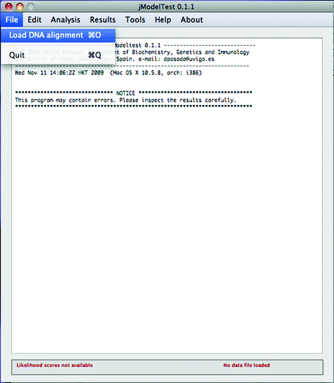
The jModelTest console.
-
2.
From the menu select “File > Load DNA alignment” and choose the FASTA format alignment that was exported from Se-Al (i.e., “H5_align_out.fas”) (see Note 8).
-
3.
Then select “Analysis > Compute likelihood scores” and a window will open with options for calculating likelihood scores.
-
4.
Change “Number of substitution schemes” to 7 and “Base tree for likelihood calculations” to BIONJ (see Fig. 3), and then click “Compute likelihoods” and a progress bar will open.
Fig. 3. 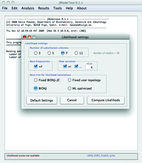
Settings for the likelihood calculations.
-
5.
The program will test 56 models in a hierarchical manner and will take approximately 20–30 min on a modern computer for an alignment of 100 full-length HA sequences. Details of the tests will also appear in the main console window (see Note 9).
-
6.
Now select “Analysis > Do AIC calculations …,” and a window will open with options for the AIC settings. Check “Write PAUP* block” and then click “Do AIC calculations” (see Fig. 4).
Fig. 4. 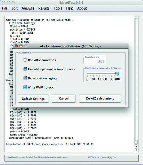
Settings for AIC model selection.
-
7.
Results of the AIC calculations will be summarized in the jModelTest console, but you will need to scroll up a bit (see Fig. 5). For the example used here, the model selected is the GTR + I + G with the precise variables defined. These variables will be used in subsequent analyses.
Fig. 5. 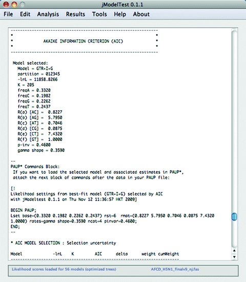
Results of the AIC model selection.
-
8.
Directly below the description of the selected model a “PAUP* Commands Block” is provided (see Fig. 5). This block will be used in Subheading 3.4.1 “Neighbor joining in PAUP*.”
-
9.
The default settings for GARLI and MrBayes use the GTR + I + G model. The execution of these programs will be described using this model. For details on using alternative models refer to the program manuals.


3.4 Phylogenetic Reconstruction
3.4.1 Neighbor Joining in PAUP*
PAUP* is one of the most widely used phylogenetic software packages. The software is not free but is powerful, flexible, and reliable. The manual included with this program contains an extensive command reference that is very useful.
-
1.
First, convert the FASTA file “H5_align_out.fas” to Nexus format using the program Se-Al, saving the file as “H5_align_out.nex” (see Subheading 3.2.2).
-
2.
Open the file “H5_align_out.nex” in a text editor, scroll to the end, and paste the “PAUP* Commands Block” from Subheading 3.3. The PAUP* block should read (see Note 10) as follows:

-
3.
This only describes the evolutionary model, so we need to include some further commands for calculating and saving the NJ tree. The PAUP* block should now read as follows:

-
4.
Make sure that the PAUP* executable and the Nexus file are contained in the home directory, although the path can be included in the execute command used in PAUP*. Please note that there is no graphical interface for the program in Mac OS X and that the UNIX version needs to be used.
-
5.
Double-click the PAUP* executable to open the program in the Terminal (see Fig. 6). At the command prompt type “execute filename.nex.” In the example used here the file name is “H5_align_out.nex.”
Fig. 6. 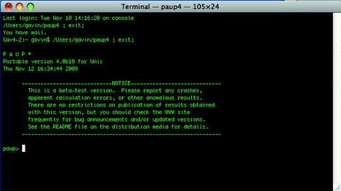
The PAUP* terminal window.
-
6.
As all the necessary commands were placed within the NEXUS file the analyses should run without any further input. Once the calculations are completed, the NJ and bootstrap trees will be saved in the same directory that contains the NEXUS file.

3.4.2 Maximum Likelihood in GARLI
Genetic algorithm for rapid likelihood inference (GARLI) performs phylogenetic searches on aligned sequence datasets using the maximum-likelihood criterion. Common substitution models are implemented in GARLI to calculate the likelihood scores. The model parameters can be fixed or estimated and used to optimize branch lengths, tree topology, and maximize the likelihood. The genetic algorithm used by GARLI to perform maximum likelihood searches is generally faster than PAUP* and, when searches have been run for sufficient length, the likelihood scores should be comparable. GARLI maximum likelihood tree search optimization is faster than PAUP* maximum likelihood analysis but slower than the neighbor joining method described above.
-
1.
For downloading, installation, and basic usage instructions please see the GARLI Web site (see Note 11).
-
2.
The best-fit evolutionary model can also be specified as a “GARLI block” in the NEXUS file; however, the format is different for the PAUP* block described above. For the model from Subheading 3.3 the GARLI block will read (see Note 12) as follows:

-
3.
So replace the PAUP* block in the NEXUS file and rename the file to “H5_align_garli.nex.”
-
4.
It is then necessary to modify the GARLI configuration file (garli.conf) to specify the analysis file. The configuration file is in the folder “example” that is included with the program download. This file can be opened in any text editor.
-
5.
On lines 2 and 6 of “garli.conf” change the field “datafname = rana.nex” to “datafname = H5_align_garli.nex” and “ofprefix = rana.nuc.GTRIG” to “ofprefix = H5.nuc.GTRIG.” This specifies the correct analysis file.
-
6.
It is also necessary to modify Lines 25–31 of the configuration file, specify that the parameters of the evolutionary model have been fixed using the GARLI block:

-
7.
It is advisable to conduct multiple runs of GARLI to ensure that an optimal result is obtained. The default is 2 replicates but this can be increased by modifying “searchreps = 2” in the configuration file.
-
8.
Ensure that the “garli.conf” file is in the same folder as the GARLI executable.
-
9.
Open the Terminal window and cd to the folder containing the executable file “Garli0.96b8.”
-
10.
Type “./Garli0.96b8” and the program will begin to run.
-
11.
Once completed, the example dataset took about 15 min, the best tree will be saved in the file “H5.nuc.GTRIG.best.tre” in the same folder. In the terminal window, the likelihood of both runs is provided, which should be similar values.
-
12.
To conduct an ML bootstrap then simply modify the third last line of the “garli.conf” file to read “bootstrapreps = 0” to “bootstrapreps = 500” or “bootstrapreps = 1,000” (see Note 13).
3.4.3 Bayesian Inference in MrBayes
MrBayes is a program for the Bayesian estimation of phylogeny. Bayesian phylogenetics has been gaining prominence and acceptance in evolutionary science, especially with dramatically improved computational power. Importantly, Bayesian phylogenetics sample many equivalent trees in the tree space in contrast to neighbor joining and maximum likelihood methods, which will produce only a single tree. The phylogenetic tree produced is based on all of these trees, which is known as the posterior probability distribution of trees. This computation is analytically difficult and for large datasets impossible. MrBayes uses a simulation method known as Metropolis-coupled Markov Chain Monte Carlo (or MCMC) to overcome this difficulty.
-
1.
For downloading, installation, and basic usage instructions please see the MrBayes Web site (see Note 14).
-
2.
The best-fit evolutionary model is specified with a “MrBayes block” in the NEXUS file; however, the format is different for the PAUP* and GARLI blocks described above. For the model from Subheading 3.3 the MrBayes block will read (see Note 15) as follows:

-
3.
Replace the PAUP* block in the NEXUS file and rename the file to “H5_align_bayes.nex.”
-
4.
Double-click the MrBayes executable file to open the program. At the prompt type “exec H5_align_bayes.nex” to execute the file (see Fig. 7).
Fig. 7. 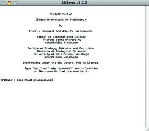
The MrBayes program window.
-
5.
The MrBayes block specified one million generations, with trees sampled every 100 generations. Also, the default setting for MrBayes is to conduct two independent runs. This will result in 10,000 trees per run, or a total of 20,000 trees.
-
6.
MrBayes will save two types of files for each independent run, the tree files and the run statistics, that have the extensions “run1.t and run2.t” and “run1.p and run2.p,” respectively.
-
7.
The Bayesian posterior probability is assessed from these trees after suboptimal trees calculated at the start of the run are discarded. The portion of the trees that are discarded are referred to as the “burnin.”
-
8.
Once the analysis has finished running, you will be prompted on whether to continue the analysis or not. First, it is necessary to check whether the two independent runs have converged by looking at the “average standard deviation of split frequencies” that is provided in the MrBayes window. As the two runs converge onto the stationary distribution, the average standard deviation of split frequencies is expected to approach zero, reflecting the fact that the two tree samples become increasingly similar. A value <0.01 is considered adequate indication that the two runs have converged.
-
9.
Alternatively, the program Tracer can be used. Double-click the Tracer icon to open the program. This has the advantage that the burnin can also be determined though visual inspection.
-
10.
Click on the “+” sign near the top left of Tracer, this will open another window to select the necessary files. Navigate to the MyBayes folder and select the run statistic files “H5_align_bayes.nex.run1.p” and “H5_align_bayes.nex.run2.p” (see Fig. 8).
Fig. 8. 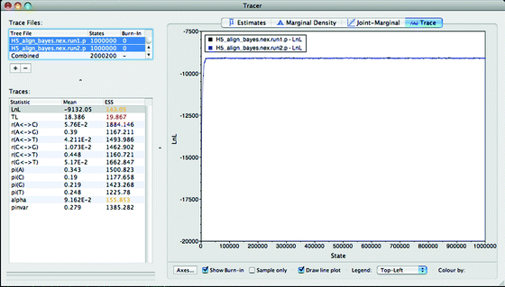
The Tracer program window.
-
11.
Tracer will automatically assign a burnin of 10%. Double-click the burnin value in the “Traces files” box and change this to zero for both files. Select both files in the “Traces files” box and then click on the LnL statistic in the “Traces” box—a graph of both tree likelihoods will appear to the right (see Fig. 8).
-
12.
For the example dataset used here, an appropriate burnin is 1,000 (10%) of sampled trees.
-
13.
If the two runs have not converged, you can continue the analysis by typing “Yes” and then entering an additional 1 million generations.
-
14.
If the two runs have converged, then type “No” and then type “sumt burnin=1,000”—or whatever burnin you have determined from visual inspection in Tracer. This will take some time and once completed, a consensus tree with Bayesian posterior probabilities will be saved as “H5_align_bayes.nex.con” (see Note 16) (Fig. 9).
Fig. 9. 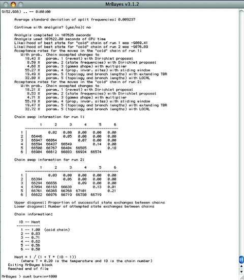
State frequencies and summarizing trees in MrBayes.


3.5 Tree Visualization with FigTree
Figtree (http://tree.bio.ed.ac.uk/software/figtree/) is a graphical viewer with various tree-editing capabilities that produces publication-quality figures in multiple graphic file formats.
-
1.
For downloading, installation, and basic usage instructions please see the Figtree Web site.
-
2.
As an example, we will use the “H5_align_bayes.nex.con” file that was generated using the sumt command in MrBayes (see Subheading 3.4.3).
-
3.
Double-click Figtree executable to start the application. To open a tree file use File > Open and then select the tree file.
-
4.
Upon opening tree files, the users are prompted to enter names for undefined labels that exist in the tree file. In this case, >95% Bayesian posterior properties are stored in the tree file (Fig. 10).
Fig. 10. 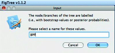
Figtree: tree input.
-
5.
The Figtree window (Fig. 11) is divided into the top menu panel, a left control panel, and the center tree panel. The top menu and the left panels can be used to edit the tree, color branches or leaves, and most importantly root the tree using an appropriate outgroup or using midpoint (see Note 17).
Fig. 11. 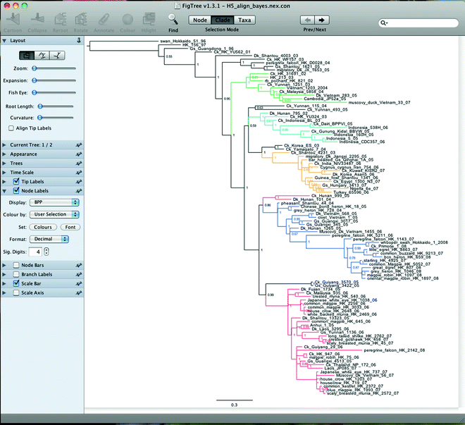
Figtree.
-
6.
Using the File > Export Graphic (or) File > Print > PDF > Save as PDF menu options the tree graphic can be exported in various graphic file formats.


4 Notes
-
1.
Other resources are available including the Influenza Research Database (http://www.fludb.org) (13) and the Influenza Primer Design Resource (http://www.ipdr.mcw.edu) (14).
-
2.
Other programs for multiple sequence alignment and optimization include ClustalW/X (15) and BioEdit (16). There are also many online alignment tools, including those provided at http://align.genome.jp/.
-
3.
Many multiple alignment programs also produce a guide tree that is used to conduct the multiple sequence alignment. This tree is unlikely to be accurate and must not be used to infer phylogenetic relationships or reproduced in publication.
-
4.
The instructions we give here are for the locally installed program; however, the program can also be run from the Web page.
-
5.
To ease the optimization of the multiple sequence alignment, shift all the sequences to the correct reading frame and translate the sequences to amino acids (select “Alignment > Alignment type > Amino Acids”).
-
6.
If you have loaded a DNA sequence alignment but wish to export the amino acid sequences, these must be converted to amino acid in the sequence inspector window first. Then, in the export file dialogue box, click the “Export alignment as viewed” tab.
-
7.
jModelTest is a Java version of the earlier ModelTest (17). There is also a MrModeltest (18) that was specifically designed for only testing those models that could be implemented in the program MrBayes. Both these programs are faster than jModeltest, but both run from the terminal window and are more difficult to use.
-
8.
jModelTest appears to have a problem loading NEXUS files. If you get an error with a particular file format, then just try a number of different file formats—as is usually the case, FASTA works fine.
-
9.
In comparison, testing 56 models using ML trees took 1 h 20 min in jModelTest. If you reduce the number of substitution schemes to 3 (i.e., 24 models) and use BIONJ trees, the analysis will run in 10–15 min.
-
10.
There is an error in the “Lset” command output from jModelTest that will cause an error when executing the file in PAUP* and other programs. Rather than having four numbers for “base = (n1 n2 n3 n4)” this should be “base = (n1 n2 n3). To fix this simply delete the last number. A similar error is made with “rmat = (n1 n2 n3 n4 n5 n6). There should only be five numbers in the “rmat” and the last number should be deleted.
-
11.
The instructions given here are for the Mac OS X Intel multithreaded v0.96, which does not have a graphical user interface, but this version is capable of distributing the analysis over multiple processors.
-
12.
In the GARLI block “e” is equivalent to “base” in the PAUP* block, “r” to “rmat,” “a” to “shape,” and “p” to “pinvar.” Details of GARLI configuration settings are available at the following site: https://www.nescent.org/wg_garli/GARLI_Configuration_Settings.
-
13.
Maximum likelihood bootstraps are very computationally intensive and even using GARLI will take days to complete 1,000 bootstraps for a dataset of 100 full-length HA genes.
-
14.
The instructions given here are for the Mac OS X executable. However, this version runs on a single processor and is quite slow. It is therefore preferable to compile the program source code on a UNIX system, as this version is capable of distributing the analysis over multiple processors.
-
15.
MrModeltest writes a MrBayes block, but jModeltest does not unfortunately. Commands for a MrBayes block are explained in detail in the MrBayes manual.
-
16.
If virus names in the NEXUS file are overly long (e.g., ≥20 characters), this may cause the sumt command to hang indefinitely.
-
17.
Extensive scientific literature illustrates the importance of using an appropriate outgroup taxon. As a rule of thumb, the best outgroup is a taxon that falls within the sister group of the ingroup under study. In the above example, for the Asian highly pathogenic avian influenza H5N1 virus ingroup, a low pathogenic H5 virus “Swan/Hokkaido/51/96” is used as an outgroup.
References
Pybus, O. G., and Rambaut, A. (2009) Evolutionary genetics of the dynamics of viral infectious disease. Nat. Rev. Genetics. 10, 540–550.
Smith, G. J. D., Vijaykrishna, D., Bahl, J., Lycett, S. J., Worobey, M., Pybus, O., Ma, S. K., Cheung, C. L., Raghwani, J., Bhatt, S., Peiris, J. S. M., Guan, Y., and Rambaut, A. (2009) Origins and evolutionary genomics of the 2009 swine-origin H1N1 influenza A epidemic. Nature 459, 1122–1125
Holmes, E. C. (ed.) (2009) The Evolution and Emergence of RNA Viruses. Oxford University Press, Oxford.
Shaw, M. L. (2007) Orthomyxoviridae: The viruses and their replication, in Fields Virology (Knipe, D. M., and Howley P. M., eds.), Lippincott Williams & Wilkins, a Wolters Kluwer Business, Philadelphia, USA.
Bao, Y., Bolotov, P., Dernovoy, D., Kiryutin, B., Zaslavsky, L., Tatusova, T., Ostell, J., and Lipman, D. (2008) The Influenza Virus Resource at the National Center for Biotechnology Information. J. Virol. 82, 596–601.
Katoh, K., Misawa, K., Kuma, K., and Miyata, T. (2002) MAFFT: a novel method for rapid multiple sequence alignment based on fast Fourier transform. Nucleic Acids Res. 30, 3059–3066.
Katoh, K., Kuma, K., Toh, H., and Miyata, T. (2005) MAFFT version 5: improvement in accuracy of multiple sequence alignment. Nucleic Acids Res. 33, 511–518.
Posada, D. (2008) jModelTest: Phylogenetic Model Averaging. Mol. Biol. Evol. 25, 1253–1256.
Swofford, D. L. (2001) PAUP*: Phylogenetic Analysis Using Parsimony (and Other Methods) 4.0 Beta. Sinauer Associates, Sunderland, MA.
Zwickl, D. J. (2006) Genetic algorithm approaches for the phylogenetic analysis of large biological sequence datasets under the maximum likelihood criterion. Ph.D. dissertation, The University of Texas at Austin.
Huelsenbeck, J. P., and Ronquist, F. R. (2001) MrBayes: Bayesian inference of phylogenetic trees. Bioinformatics 17, 754–755.
Maddison, D. R., Swofford, D. L., and Maddison, W. P. (1997) NEXUS: an extensible format for systematic information. Syst. Biol. 46, 590–621.
Squires, B., Macken, C., Garcia-Sastre, A., Godbole, S., Noronha, J., Hunt, V., Chang, R., Larsen, C. N., Klem, E., Biersack, K., and Scheuermann, R. H. (2008) BioHealthBase: informatics support in the elucidation of influenza virus host pathogen interactions and virulence. Nucleic Acids Research 36, D497–D503..
Bose, M. E., Littrell, J. C., Patzer, A. D., Kraft, A. J., Metallo, J. A., Fan, J., and Henrickson, K. J. (2008) The Influenza Primer Design Resource: a new tool for translating influenza sequence data into effective diagnostics. Influenza Other Respi Viruses. 2, 23–31.
Thompson, J. D., Higgins, D. G., and Gibson, T. J. (1994) CLUSTAL W: improving the sensitivity of progressive multiple sequence alignments through sequence weighting, position specific gap penalties and weight matrix choice. Nucl. Acids Res. 22, 4673–4680.
Hall, T. A. (1999) BioEdit: a user-friendly biological sequence alignment editor and analysis program for Windows 95/98/NT. Nucl. Acids. Symp. Ser. 41, 95–98.
Posada, D., and Crandall, K. A. (1998) Modeltest: testing the model of DNA substitution. Bioinformatics 14, 817–818.
Nylander, J. A. A. (2004) MrModeltest, version 2. Program distributed by the author. Evolutionary Biology Centre, Uppsala University.
Acknowledgments
G.J.D.S. is supported by a career development award under National Institutes of Health, National Institute of Allergy and Infectious Disease contract HHSN266200700005C and G.J.D.S., J.B. and D.V. by the Duke–NUS Signature Research Program funded by the Agency for Science, Technology and Research, and the Ministry of Health, Singapore.
Author information
Authors and Affiliations
Corresponding author
Editor information
Editors and Affiliations
Rights and permissions
Copyright information
© 2012 Springer Science+Business Media, LLC
About this protocol
Cite this protocol
Smith, G.J.D., Bahl, J., Vijaykrishna, D. (2012). Genetic Analysis. In: Kawaoka, Y., Neumann, G. (eds) Influenza Virus. Methods in Molecular Biology, vol 865. Humana Press. https://doi.org/10.1007/978-1-61779-621-0_13
Download citation
DOI: https://doi.org/10.1007/978-1-61779-621-0_13
Published:
Publisher Name: Humana Press
Print ISBN: 978-1-61779-620-3
Online ISBN: 978-1-61779-621-0
eBook Packages: Springer Protocols