Next-Generation Sequencing for Porcine Coronaviruses

Abstract

The outbreak of porcine epidemic diarrhea virus and the discovery of porcine deltacoronavirus in the USA have led to multiple questions about the evolution of coronaviruses in swine. Coronaviruses are enveloped virus, containing a positive-sense single-stranded RNA genome (26–30 kb) that can cause respiratory or enteric illness in swine. With current technologies, the complete viral genomes can be determined to understand viral diversity and evolution. In this chapter, we describe a method to deep genome sequence porcine coronavirus on the Illumina MiSeq, avoiding the number of contaminating reads associated with the host and other microorganisms.

1 Introduction

Coronaviruses (CoVs) have negatively impacted the health of pigs for multiple decades [1]. Currently, five swine CoVs have been identified: transmissible gastroenteritis virus (TGEV), porcine respiratory coronavirus (PRCV), porcine epidemic diarrhea virus (PEDV), hemagglutinating encephalomyelitis virus (HEV), and porcine deltacoronavirus (PDCoV) [2, 3]. Multiple studies have described methods to detect CoVs by PCR methods [4–7]. In addition, multiple manuscripts have described Sanger sequencing methodologies to investigate the genetic diversity and evolution of individual or partial CoV genes [7–9]. However, investigating partial genome of these CoVs underestimates the evolutionary history of these viruses [10].

In the pursuit to investigate recombinant regions within the CoV genome and to further enhance our understanding of CoV evolution, CoV genome sequencing has become very valuable. In addition, next-generation sequencing (NGS ) technology has facilitated the use of complete genomic sequencing with extreme high coverage and reduced the cost compared to Sanger sequencing. Many laboratories have purchased desktop NGS sequencers to expand their sequencing capabilities, due to the relatively low cost associated with the equipment. However, achieving viral genomes directly from samples can be difficult since the total RNA, including mRNA from host cells and bacteria, is also sequenced [11–13]. Nevertheless, NGS technology is a very powerful tool in generating CoV genomes, which could lead to a better understanding of CoV evolution.

2 Materials

2.1 Sample Handling and RNA Extraction

• 1. Phosphate-buffered solution (PBS).

• 2. Stomacher^® 400 Circulator (Laboratory Supply Network, USA).

• 3. 1 mL Syringe without needle.

• 4. 0.22 μm Syringe filters.

• 5. Turbo DNA (Thermo Fisher Scientific, USA).

• 6. RNase ONE™ Ribonuclease (Promega, USA).

• 7. MagMAX™-96 Viral RNA Isolation Kit (Thermo Fisher Scientific, USA). Store the buffers at room temperature, the RNA-binding beads at 4 °C, and carrier RNA and binding enhancer at −20 °C.

2.2 Evaluation and Assessment of RNA Mass Using Ribogreen and Agilent Bioanalyzer

• 1. Quant-iT™ RiboGreen^® RNA Assay Kit (Life Technologies, USA).

• 2. FLx800 Fluorescence Reader or similar UV-V reader (Bio-Tek, USA).

• 3. λ RNA Standard (Life Technologies, USA).

• 4. Black 96-well plate (Thermo Fisher Scientific, USA).

• 5. Agilent RNA 6000 Nano kit (Agilent, USA).

• 6. Molecular-grade water (Sigma-Aldrich, USA).

2.3 Illumina TruSeq RNA Library Creation and Validation

• 1. TruSeq RNA Sample Preparation Kit, Box A (Illumina, USA).

• 2. TruSeq RNA Sample Preparation Kit, Box B (Illumina, USA).

• 3. TruSeq RNA Sample Preparation Kit, PCR Prep Box (Illumina, USA).

• 4. SuperScript II (Life Technologies, USA).

• 5. AmPure XP beads (Beckman Coulter, USA).

• 6. Ethanol, 200 proof (Sigma-Aldrich, USA).

• 7. Microseal “B” adhesive seals (BioRad, USA).

• 8. RNase/DNase-free strip tubes and caps.

• 9. Thermal Scientific PCR plates (Life Technologies, USA).

• 10. BioRad PCR plates (BioRad, USA).

• 11. Magnetic plate or stand (Life Technologies, USA).

• 12. Qiagen EB Buffer (Qiagen, USA).

2.4 Sequencing on the Illumina Miseq

• 1. MiSeq Reagent Kit v2 (Illumina, USA).

• 2. PhiX Control (Illumina, USA).

• 3. 2 nM Normalized libraries.

• 4. Stock 1.0 N NaOH (Illumina, USA).

• 5. Tris-Cl, 10 mM, pH 8.5 (Qiagen, USA).

2.5 Sequence Assembly

• 1. Trimmomatic.

• 2. DNASTAR software package.

3 Methods

3.1 Sample Handling and RNA Extraction

• 1. Fecal swabs: Place the swab into a tube containing 2 mL of PBS. Vortex the sample in the solution for 30 s. Centrifuge the sample for 20 min at 3000 × g. Transfer the supernatant to a new tube, and store the sample at −80 °C.

• 2. Feces : Weigh 1 g of feces and place the feces into a tube containing 3 mL of PBS. Vortex the sample in the solution for 30 s. Centrifuge the sample for 20 min at 3000 × g. Transfer the supernatant to a new tube, and store the sample at −80 °C.

• 3. Tissues: Weigh 1 g of the tissue and place the gram in 3 mL of PBS. Homogenize the tissue for 1 min. Transfer the supernatant to a new tube, and centrifuge the sample for 20 min at 3000 × g. Transfer the supernatant to a new tube, and store the sample at −80 °C.

• 4. Using a syringe, aspirate the supernatant from each sample and pass the sample through a 0.22 μm filter into a new tube (see Note 1 ).

• 5. After the samples have been filtered, in a separate tube add:

  • (a) 20 μL of 10× Turbo DNase Buffer.

  • (b) 12 μL of Turbo DNase.

  • (c) 2 μL of RNase ONE Ribonuclease.

  • (d) 200 μL of filtered sample.

• 6. Mix the sample and reagents gently with the pipette or lightly vortex mixture.

• 7. Incubate the samples for 37 °C for 90 min, and immediately proceed to the extraction to inactivate the DNase and RNase.

• 8. Extract the RNA from the treated samples using the MagMAX™-96 Viral RNA Isolation Kit. Store the extracted RNA (40 μL) at −80 °C.

3.2 Evaluation and Assessment of RNA Mass Using Ribogreen and Agilent Bioanalyzer

• 1. Quantify the RNA using the Quant-iT™ RiboGreen^® RNA Assay Kit, according to the manufacturer’s instructions (see Note 2 ).

• 2. Once the concentration of RNA has been determined, assess the RNA integrity using the Agilent Bioanalyzer, according to the manufacturer’s instructions (see Note 3 ).

3.3 Illumina TruSeq RNA Library Creation and Validation

• 1. Follow the manufacturer’s protocol for TruSeq RNA Library Preparation Kit v2 as recommended, with the following modification (see Note 4 ).

• 2. Normalize Ribogreen quantitated RNA samples to 20 ng/μL with water, for an input mass of 100 ng per reaction. If starting RNA of 20 ng/μL is unavailable, use a maximum of 5 μL purified sample to start the elute, prime, and fragment steps.

• 3. Shorten RNA fragmentation time to 2 min to keep the fragments as long as possible to take advantage of the sequencing length obtained using MiSeq 2 × 250 bp run.

• 4. Validate the library yield using a fluorometric assay, either PicoGreen or Qubit, according to the manufacturer’s instructions (see Note 5 ).

• 5. Normalize libraries to 10 nM using Qiagen EB buffer or standard Tris buffer. If final undiluted library concentrations are below 10 nM, normalize to 2 nM.

3.4 Sequencing on the Illumina MiSeq

• 1. Combine equal volumes of 10 or 2 nM normalized libraries depending on the type of MiSeq run required for sample number.

• 2. Denature and dilute libraries to 8 pM for sequencing with 1 % PhiX spike.

• 3. Sequence pooled libraries using a MiSeq Nano 250 bp PE (MiSeq 500 cycle v2 Nano) run if sequencing less than two libraries (see Note 6 ).

• 4. Load instrument according to the manufacturer’s specifications.

3.5 Sequence Assembly (See Note 7 )

• 1. Transfer the fastq from the MiSeq machine. The fastq files will need to undergo a quality assurance to remove adapter sequences and low-quality read, which can be done with Trimmomatic, an open-source software[14] (see Note 8 ).

• 2. Reference-based assembly for coronavirus genomes.

  • (a) Open the SeqManNGen program, select reference-based assembly, and load the reference CoV genome and the correlating paired fastq files to the sample and run the assembly.

  • (b) Evaluate assembly of reads (see Note 9 ). If there are regions with minimal coverage, this indicates that the reads do not match the reference sequence. Remove the reference strain and split the contig at the low-coverage regions. Trim the 5′ and 3′ regions of the new contigs at the split region.

  • (c) Preform reference-based assembly with the newly generated contigs. The contig ends will extend with the viral reads.

  • (d) Merge the contigs together to generate a single contig.

  • (e) Remap the reads to the contig to verify accurate generation of the viral genome and sufficient coverage. The contig can be saved as a fasta file for future phylogenetic analysis.

• 3. De novo assembly for viral genomes.

  • (a) Open the SeqManNGen program, select reference-based assembly, and load the Susscrofa genome and the correlating paired fastq files to the sample. In the advance options, select saved unmapped reads, which will save the reads that did not map to Sus scrofa genome once the assembly has finished. Run the assembly.

  • (b) After the program finished running, open SeqManNGen program again, select de novo assembly, and load the unassembled fastq file from the previous reference-based assembly.

  • (c) Once the de novo assembly has finished, BLAST the contigs to locate the designated coronavirus contigs.

  • (d) Remap the reads to the coronavirus sequence and verify accurate and sufficient coverage. The contig can be saved as a fasta file for future phylogenetic analysis.

4 Notes

• 1. Some samples may contain excess organic material and clog the filter. If this occurs, centrifuge the sample for another 20 min at 3000 × g.

• 2. Quantification needs to occur with a fluorometry system that measures only single-stranded nucleic acids and is insensitive to organic contaminants commonly used in extraction kits, which allows for more accurate quantification of input mass and higher probability of successful library preparation.

• 3. The RNA sample needs to be assessed for the concentration of host ribosomal RNA (rRNA). This assessment does not remove host rRNA, but ensures that the RNA is free of rRNA, which severely dilutes the number of viral reads (Fig. 1).

  Fig. 1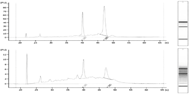

  

  Example of rRNA contamination. The Agilent traces are indicative of incomplete viral RNA purification with 18S and 28S host rRNA peaks

• 4. The mRNA purification strategy should be skipped since the oligo-dT-coated magnetic beads were used to specifically bind poly-A-tailed mRNA. The viral RNA will not be poly-A tailed. Start the library preparation at step “Incubate RFP,” which is the start of random primed cDNA synthesis.

• 5. Typical concentrations of viral RNA libraries for the TruSeq RNA library preparation kit are 1–15 ng/μL.

• 6. The concentration of coronavirus must be estimated by RT-PCR . However, the concentration by RT-PCR may not indicate successful generation of the complete viral genome since total RNA was used in the library preparation. Generally, lower concentration of viral particles by RT-PCR indicates that more reads are needed to generate a complete genome. If libraries have limited host contamination and have an acceptable concentration of viral RNA (Ct value <25), a 1 million read output per sample should be sufficient for assembly. If more reads are needed per sample, the MiSeq v2 250 PE kit can be used.

• 7. Two major assembly methodologies are available, reference based and de novo assembly. However, due to the genetic diversity of viruses, gaps in coverage can occur during reference-based assembly. We will briefly discuss both options in this chapter. Reference-based assembly maps the MiSeq reads to a known sequence (template) to build a contig while de novo assembly does not use a sequence to build a contig, which take longer to run. Since the MiSeq generates reads from total RNA, host reads need to be removed to facilitate de novo assembly, which can be done by first mapping the reads to the swine genome and saving the unmapped reads. Hence, the de novo assembly process described here first utilizes a reference-based assembly (to remove host reads) and then a de novo assembly to construct contigs.

• 8. Many different programs are available to remove adapter sequences and low-quality read and assembly genomes, and each program uses slightly different algorithms and operations to accomplish this task. Removing low-quality reads is necessary before attempting viral assembly.

• 9. Coverage across the genome will vary and is expected. The valleys, which indicate less coverage, should have approximately the same amount of coverage (Fig. 2a). If valleys with less coverage are comparable to the other valleys with high coverage, the reads did not match to the reference due to genetic diversity of the CoV strain (Fig. 2b).

  Fig. 2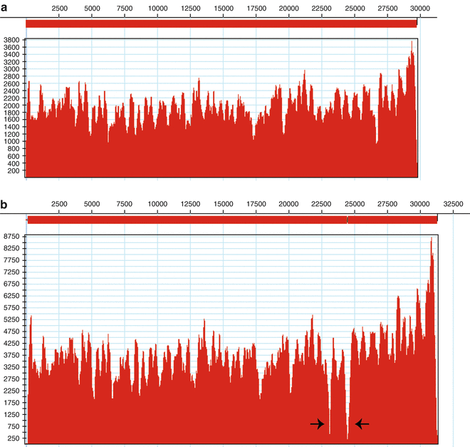

  

  Examples of reads mapping to reference genome. The x-axis represents the length of the genome while the y-axis represents depth of coverage. (a) Unequal coverage across the genome. (b) Gaps in coverage due to genetic differences between the reference genome and sequenced sample, indicated by the black arrows

References

Saif L, Pensaert MB, Sestak K, Yeo S, Jung K (2012) Diseases of swine. In: Zimmerman JJ, Ebrary I (eds) Coronaviruses, 10th edn. Wiley-Blackwell, Chichester, West Sussex, pp 501–524
Masters P, Perlman S (2013) Fields virology. In: Fields BN, Knipe DM, Howley PM, Ebrary I (eds) Coronaviridae, 6th edn. Wolters Kluwer Health/Lippincott Williams & Wilkins, Philadelphia, pp 825–858
Woo PC, Lau SK, Lam CS, Lau CC, Tsang AK, Lau JH, Bai R, Teng JL, Tsang CC, Wang M, Zheng BJ, Chan KH, Yuen KY (2012) Discovery of seven novel Mammalian and avian coronaviruses in the genus deltacoronavirus supports bat coronaviruses as the gene source of alphacoronavirus and betacoronavirus and avian coronaviruses as the gene source of gammacoronavirus and deltacoronavirus. J Virol 86:3995–4008. doi:10.1128/JVI.06540-11
Marthaler D, Raymond L, Jiang Y, Collins J, Rossow K, Rovira A (2014) Rapid detection, complete genome sequencing, and phylogenetic analysis of porcine deltacoronavirus. Emerg Infect Dis 20:1347–1350. doi:10.3201/eid2008.140526
Zhao J, Shi BJ, Huang XG, Peng MY, Zhang XM, He DN, Pang R, Zhou B, Chen PY (2013) A multiplex RT-PCR assay for rapid and differential diagnosis of four porcine diarrhea associated viruses in field samples from pig farms in East China from 2010 to 2012. J Virol Methods 194:107–112. doi:10.1016/j.jviromet.2013.08.008
Rodriguez E, Betancourt A, Relova D, Lee C, Yoo D, Barrera M (2012) Development of a nested polymerase chain reaction test for the diagnosis of transmissible gastroenteritis of pigs. Rev Sci Tech 31:1033–1044
Costantini V, Lewis P, Alsop J, Templeton C, Saif LJ (2004) Respiratory and fecal shedding of porcine respiratory coronavirus (PRCV) in sentinel weaned pigs and sequence of the partial S-gene of the PRCV isolates. Arch Virol 149:957–974. doi:10.1007/s00705-003-0245-z
Li R, Qiao S, Yang Y, Su Y, Zhao P, Zhou E, Zhang G (2014) Phylogenetic analysis of porcine epidemic diarrhea virus (PEDV) field strains in central China based on the ORF3 gene and the main neutralization epitopes. Arch Virol 159:1057–1065. doi:10.1007/s00705-013-1929-7
Sun R, Leng Z, Zhai SL, Chen D, Song C (2014) Genetic variability and phylogeny of current Chinese porcine epidemic diarrhea virus strains based on spike, ORF3, and membrane genes. Sci World J 2014:208439. doi:10.1155/2014/208439
Vlasova AN, Marthaler D, Wang Q, Culhane MR, Rossow KD, Rovira A, Collins J, Saif LJ (2014) Distinct characteristics and complex evolution of PEDV strains, North America, May 2013-February 2014. Emerg Infect Dis 20:1620–1628. doi:10.3201/eid2010.140491
Belak S, Karlsson OE, Blomstrom AL, Berg M, Granberg F (2013) New viruses in veterinary medicine, detected by metagenomic approaches. Vet Microbiol 165:95–101. doi:10.1016/j.vetmic.2013.01.022
Hall RJ, Wang J, Todd AK, Bissielo AB, Yen S, Strydom H, Moore NE, Ren X, Huang QS, Carter PE, Peacey M (2014) Evaluation of rapid and simple techniques for the enrichment of viruses prior to metagenomic virus discovery. J Virol Methods 195:194–204. doi:10.1016/j.jviromet.2013.08.035
Shah JD, Baller J, Zhang Y, Silverstein K, Xing Z, Cardona CJ (2014) Comparison of tissue sample processing methods for harvesting the viral metagenome and a snapshot of the RNA viral community in a turkey gut. J Virol Methods 209:15–24. doi:10.1016/j.jviromet.2014.08.011
Bolger AM, Lohse M, Usadel B (2014) Trimmomatic: a flexible trimmer for Illumina sequence data. Bioinformatics 30:2114–2120. doi:10.1093/bioinformatics/btu170
Author information
Authors and Affiliations
Corresponding author
Editor information
Editors and Affiliations
Rights and permissions
Copyright information
© 2016 Springer Science+Business Media New York
About this protocol
Cite this protocol
Marthaler, D., Bohac, A., Becker, A., Peterson, N. (2016). Next-Generation Sequencing for Porcine Coronaviruses. In: Wang, L. (eds) Animal Coronaviruses. Springer Protocols Handbooks. Humana Press, New York, NY. https://doi.org/10.1007/978-1-4939-3414-0_19
Download citation
DOI: https://doi.org/10.1007/978-1-4939-3414-0_19
Published:
Publisher Name: Humana Press, New York, NY
Print ISBN: 978-1-4939-3412-6
Online ISBN: 978-1-4939-3414-0
eBook Packages: Springer Protocols