Investigating Diffusion Dynamics and Interactions with Scanning Fluorescence Correlation Spectroscopy (sFCS)

Abstract

Activation of immune cells and formation of immunological synapses (IS) rely critically on the reorganization of the plasma membrane. These highly orchestrated processes are driven by diffusion and oligomerization dynamics, as well as by single molecule interactions. While slow macro- and meso-scale changes in organization can be observed with conventional imaging, fast nano-scale dynamics are often missed with traditional approaches, but resolving them is, nonetheless, essential to understand the underlying biological mechanisms at play. Here, we describe the use of scanning fluorescence correlation spectroscopy (sFCS) and scanning fluorescence cross-correlation spectroscopy (sFCCS) to study reorganization and changes in molecular diffusion dynamics and interactions during IS formation and in other biological settings. We focus on the practical aspects of the measurements including calibration and alignment of the optical setup, present a comprehensive protocol to perform the measurements, and provide data analysis pipelines and strategies. Finally, we show an exemplary application of the technology to studying Lck diffusion during T-cell signaling.

1 Introduction

Cells are complex biological systems maintained and controlled by the rapid movement of biomolecules within and between cellular compartments. These molecules are traditionally studied isolated from cellular context, either purified from native environments, recombinantly produced, or in a chemically fixed state in which dynamics are lost. However, complex cellular programs, like the formation of immune synapses (IS) between T cells and their targets [1, 2], are driven by the concerted effort of a variety of groups of molecules that exhibit a range of diffusion dynamics (Fig. 1a). Mature IS are organized into molecular compartments, called supramolecular activation clusters (SMACs), that partition the cell into constrained domains into which surface proteins are sorted based on size and F-actin-mediated transport [2]. These compartments are heterogeneous and crowded [3,4,5,6], which has made it challenging to dissect ensemble protein dynamics at the cell-cell interface. In this chapter, we describe how a specialized form of fluctuation analysis, scanning fluorescence correlation spectroscopy (sFCS), can be used to study a wide range of molecular diffusion dynamics in live cells (Fig. 1b) [7]. sFCS can be performed in dense protein environments (10²–10³ molecules∙μm⁻²) like the cell surface and exhibits less photobleaching effects compared to conventional FCS methods [8]. Spatial information can also be obtained at a resolution capable of differentiating between cellular structures or compartments (~0.1 μm, e.g., SMACs) [9].

Fig. 1

Dynamics and molecular reorganization at the IS. a. Top-down view of a classical T cell immune synapse (inset shows zy-profile view) with zones of different molecular organization color-coded (magenta, dSMAC; blue, pSMAC; yellow, cSMAC). Examples of proteins with reported diffusion coefficients, D, and dynamic properties are shown on the right [55,56,57,58,59,60,61]. b. Spectrum of diffusion coefficients for biomolecules adapted from Cell Biology by the Numbers [7]. Note that the diffusion coefficients shown for each class of biomolecule span both in vitro and in situ environments. The suitable range for scanning FCS (sFCS) and conventional point FCS (pFCS) is indicated above the spectrum. The line-scanning mode extends the lower limit of diffusion speeds that can be measured with FCS, but restricts the measurement of fast-moving molecules

FCS was originally devised in the 1970s but has become increasingly relevant in biological research over the past decades, especially with the increasing availability of commercial turn-key instrumentation and the development of genetically encodable bright fluorescent labels that enable tagging of endogenous proteins [10,11,12,13,14]. In addition to simple measurements of diffusion (transit times), FCS also offers direct insight into molecular behavior and organization in the form of oligomerization, concentration, anomalous diffusion, and heterotypic interactions [15, 16]. The basis for most FCS acquisition is a conventional confocal microscope, and the introduction of confocal optics ultimately allowed FCS acquisitions as we know them today [17, 18]. The key feature of a confocal microscope, the pinhole, together with focused laser beams allow fluorescence detection to be constrained to a small femtolitre-sized volume (Fig. 2a,b). Fluorescent molecules that enter and leave the excitation volume cause intensity fluctuations on the detectors. These intensity fluctuations (or, at very low concentrations, single molecule bursts) are related to the average time molecules spend crossing the observation volume, the transit time, τ_D [17]. In standard, single-point FCS (pFCS), this observation volume is stationary, and thus dynamics are only sampled at one point in space. sFCS has been developed to overcome this limitation and to provide a spatial dimension for diffusion measurements [19]. Using a fast galvometric scanner (in a laser scanning microscope (LSM)), the focus can be scanned rapidly a long a line (or circle) and thus multiple fluctuation measurements obtained across space [8, 20, 21] (Fig. 2b). Though no hardware modifications to the LSM are required to perform sFCS [9], it is advantageous to use highly sensitive single-photon avalanche diodes (SPADs) or hybrid detectors capable of operating in photon counting mode for fluorescence detection.

Fig. 2

Fluorescence correlation spectroscopy at a laser scanning microscope. a. Schematic of an inverted laser scanning microscope with two excitation lasers and two detectors. b. Molecular diffusion dynamics sampled by point FCS (left) and scanning FCS (right). Molecular motion (diffusion) of fluorescing molecules (green) cause intensity fluctuations over time in the respective excitation volumes (blue and magenta). c. Auto-correlation curves illustrating the information contained in fluctuation experiments. The decay time (transit time, τ_D, left) relates to the diffusion coefficient and displays the average time a molecule needs to cross the observation area/volume. The amplitude (right) of auto-correlation curves relates inversely to the average number of molecules in the focus, N (which can also be expressed as concentration for known observation volume). d. In sFCS, the auto-correlation curves are calculated for every location along the scanned line resulting in an array of curves mapped across space (left). For simplification, the 3D curves are often represented in a so-called 2D correlation carpet (right). Normalized correlation is color-coded as indicated from blue to red, and the transit time (characteristic decay time) can be read from the green/yellow shaded area. e. Scanning FCS data can be acquired in two channels by simultaneously scanning, for example, blue and red excitation beams across space. Fluorescence intensity for every scanned point is recorded in two channels (green fluorescence in CH0 and far-red fluorescence in CH1, respectively). f. Two-color fluorescence fluctuation acquisitions allow to calculate auto-correlation curves (red and green) for the two fluorescence intensity channels (CH0 and CH1) as well as their cross-correlation (CC, grey). Molecules that move independently can be analyzed by auto-correlation but do not cause a positive cross-correlation amplitude (left). Co-diffusing molecules, interacting molecules, can be identified by a positive cross-correlation amplitude (right)

The intensity fluctuations generated in routine FCS data acquisition can be analyzed with many different fluctuation spectroscopy algorithms [15, 22,23,24], but here we focus only on the use of auto- and cross-correlation analysis. In simple terms, the correlation analysis evaluates the self-similarity of the signal at different time delays (lag times, τ) as a temporal average for every point in time which produces a characteristic decay curve. This curve, the auto-correlation function (ACF), carries information about molecular dynamics and concentration (Fig. 2c) [25] which can be extracted by fitting the data to an appropriate physical model. The decay time of the curve relates to the average time the fluorescent molecules need to cross the confocal volume, and the amplitude is inversely proportional to the average number of particles in focus. In sFCS, this information can then be mapped across space and is often represented as a correlation carpet (Fig. 2d). Crucially, for measurements in live cells, acquisition through sFCS greatly reduces phototoxicity and photobleaching effects since the excitation spot only resides for a few microseconds in any given location and allows sampling of a larger ensemble of molecules [9]. We focus here on the acquisition of sFCS data in the plane of the membrane. However, scanning fluctuation data can also be acquired perpendicular to the membranes (i.e., in the equatorial plane of cells or vesicles). In this case the spatial information allows to correct for motion of the membrane [20, 26].

Intensity fluctuations across space can analogously be acquired in two channels (Fig. 2e) allowing users to analyze co-diffusion of two different labels, for example, GFP and RFP [20, 26, 27]. As in single color acquisitions, analyzing the auto-correlation of the channels separately yields information on diffusion dynamics and concentration of the two labels. Cross-correlation analysis (correlating CH0 with CH1) allows for the direct and absolute quantification of molecular interactions, i.e., co-diffusion (Fig. 2f). The amplitude of the cross-correlation function (CCF) is directly proportional to the fraction of co-diffusing species (e.g., green-red heterodimers) in the observation volume [28]. Unlike the ACF, a higher amplitude of the CCF indicates more interacting molecules and not a lower concentration.

Overall, sFCS and sFCCS measurements have proven useful tools for probing molecular organization at the plasma membrane of living cells and beyond. In this chapter, we present the hardware requirements, the calibration strategies, the acquisition parameters, and the analysis strategies for spatially resolved fluctuation data. Furthermore, we provide a guide for troubleshooting and potential downstream analysis.

2 Materials

2.1 Hardware and Software

• 1. Confocal LSM (Zeiss780/880/980, Leica SP8, Abberior, PicoQuant MicroTime 200 or comparable) (see Notes 1–3).

• 2. Microscope control software (Zen, LAS-X or generic).

• 3. FoCuS_scan (https://github.com/dwaithe/FCS_scanning_correlator/releases/tag/1.15.107).

2.2 Calibration and Alignment

• 1. Chambered glass coverslip: e.g., Ibidi μ-Slide 8-well with #1.5 glass or equivalent.

• 2. 20 nM Alexa 488® dye in water.

• 3. 10 nM Rhodamine B in water.

• 4. 10 nM Tandem dye labeled oligonucleotide as cross-correlation positive control (e.g., see [29]).

• 5. TetraSpeck beads from ThermoFisher Scientific catalogue #T7279 or equivalent.

2.3 Model Membrane Sample Preparation

• 1. HEPES-buffered saline (HBS): 1.0 g/L dextrose, 5 g/L HEPES, 0.37 g/L KCl, 8 g/L NaCl, 0.13 g/L Na₂HPO₄.2H₂O, pH 7.2 supplemented with 0.1% human serum albumin (HSA), 1 mM CaCl₂ and 2 mM MgCl_2.

• 2. 5% Bovine serum albumin (BSA).

• 3. 10 mM Nickel sulfate (NiSO₄).

• 4. DOPC and DOGS-NTA liposome preparations [30,31,32].

• 5. Cleanroom-grade glass coverslips D623 25 x 75 mm #1.5H (Nexterion or equivalent).

• 6. Sticky-slide VI 0.4 adhesive chamber (Ibidi or equivalent).

• 7. Chloroform.

• 8. 300 mM sucrose in water.

• 9. Phosphate-buffered saline (PBS).

• 10. Platinum wire (Pt wire, 0.5 mm diameter).

• 11. Function generator with BNC to crocodile clamp adaptors.

2.4 Live Cell Samples

• 1. Human embryonic kidney 293 T cells (HEK293T, ATCC or authenticate).

• 2. Dulbecco’s Modified Eagle’s Medium (DMEM) supplemented with 10% fetal bovine serum (v/v), 1% penicillin/streptomycin.

• 3. Trypsin 10x solution: 2.5% 1:250 Trypsin in Hanks’ Balanced Salt Solution.

• 4. GeneJuice® (Merck) or similar transfection reagent.

3 Methods

3.1 Microscope Calibration Using Point FCS in Solution

• 1. Calibrate the system at the beginning of each experimental session by measuring the ACF of a dye in aqueous solution with a known concentration and diffusion coefficient (see Notes 3 and 4). This is important for obtaining high-quality fluctuation data, especially in biologically complex samples such as live cells. The chosen dye(s) should have spectral properties similar to the fluorochrome in the sample (e.g., use Alexa Fluor 488 to calibrate the 488 nm line to excite EGFP; see Note 5). This also allows for the size of the beam waist to be determined which is necessary for calculating diffusion coefficients and the absolute concentration of fluorophores (see Sect. 3.9.2). Calibration is performed with the pFCS software module which provides important photon-counting parameters (e.g., count rate, counts per molecule (CPM)) in addition to protocols for aligning the pinhole to maximize signal. In principle, pFCS can also be performed without a dedicated software module by acquiring fluorescence over time in a single pixel.

• 2. Ensure the correction collar is rotated to match the thickness of the glass coverslip (0.17 mm) such that the black line (25 °C) or orange line (37 °C) is lined up with this value (Fig. 3a).

• 3. Load a dye solution onto a chambered glass coverslip (see Note 5), and prepare an appropriate optical setup to illuminate the sample (e.g., 20 nM Alexa Fluor 488 solution measured on a Zeiss LSM system with 488 nm laser excitation, Channel S acquisition, multiple beam splitter (MBS) 488 also known as dichroic mirror).

• 4. Adjust the focus of the LSM such that the focal plane is above the glass surface (about 30 μm in solution).

• 5. Navigate to the FCS tab of the microscope, and open the “Count Rate” panel, making a note of the current count rate.

• 6. Slowly rotate the correction collar on the objective until the count rate and cpm are at their maximum. This adjustment is to correct for small variations in glass thickness. Unadjusted correction collars can impair the quality of the correlation curves recorded, dampening the correlation amplitude and increasing noise (Fig. 3b).

• 7. Navigate to the pinhole adjustment protocol, and make sure the pinhole is set to 1 airy unit (AU). Choosing the right size of pinhole is important as otherwise not enough light or too much (out-of-focus) light is collected (Fig. 3c).

• 8. Aligning the pinhole position is required to maximize signal to noise ratio (SNR). Select “Coarse” for x-adjustment. Wait until the adjustment has found the maximal count rate. Repeat for y-adjustment.

• 9. Repeat step 7 but using the “Fine” option for precise alignment of the pinhole. Figure 3d, e, f illustrates the effect of pinhole positioning (see Note 6).

• 10. The microscope is now ready for FCS measurements. Test this by acquiring point-FCS measurements of the dye solution (e.g., three repeats of 10 seconds) which should generate characteristic auto-correlation decay curves (Fig. 3b). It is advisable to keep a record of the calibrations over time to ensure that the measurements from different days are comparable and that the performance of the microscope does not drift (e.g., laser power constantly dropping would cause constant decrease of cpm).

• 11. pFCS measurements can be fitted at the LSM or exported for fitting in external software to obtain τ_D which is used to calculate the size of the observation volume (see Sect. 3.9.2).

Fig. 3

Checking alignment of the confocal microscope using pFCS acquisitions: Effect of the correction collar as well as the pinhole size and position a. Schematic illustrating the influence of the correction collar ring on the sharpness of the point-spread-function (PSF). b. Experimental auto- and cross-correlation curves obtained from a solution containing two dyes (Alexa Fluor 488 and Abberior STAR Red, green and red channel, respectively) at correct positioning of the correction collar (around 0.17 for #1.5 glass, left) versus incorrect position of the correction ring (right). c. Effect of the pinhole size on the FCS curve shape and quality of an example measurement of Abberior STAR Red excited at 633 nm (10 s acquisition time). At open pinhole (blue dots) too much light (out-of-focus) is collected dampening the correlation amplitude. With a closed pinhole not enough light to obtain a correlation curve is obtained (red dots). The inset shows an approximation of the airy function (x section of the airy disk of a point emitter). The dashed lines indicate choice of pinhole size (too small, red, or too large, blue). The magenta dashed line indicates 1 airy unit which is the typical choice for confocal imaging and FCS. d. Schematic of the procedure to align the pinhole in the emission path. The position of the pinhole can be moved in x and y to optimize light throughput (note only x alignment is shown). e. Fitting parameters (Number of Particles, N, brightness, cpm) from FCS curves at various x-positions of the pinhole for measurements of Alexa Fluor 488 (20 nM in water) excited with 488 nm measured on a Zeiss 880. f. Respective FCS auto-correlation curves at different pinhole positions for some of the data points in panel e

3.2 Fluorophore Optimization with FCS Excitation Scans

• 1. Each new dye, probe, or fluorescent protein (FP) should be characterized for its use with FCS before starting the experiments. Data quality mainly depends on the brightness of the fluorophore, i.e., cpm [33]. Brightness increases with laser power, so it is important to reach powers sufficient to produce signals of good quality (i.e., large intensity fluctuations). However, photobleaching and optical saturation effects negatively affect measurements and bias the fitting parameters when laser power is too high [33,34,35].

• 2. As for the calibration above (Sect. 3.1), use a dye on cover glass and set up appropriate optics. FCS excitation scans can also be performed in the actual sample, e.g., on fluorescent proteins expressed in cells.

• 3. Acquire pFCS data at increasing laser powers (e.g., 1 μW, 2.5 μW, 5 μW, 10 μW, 25 μW). Monitor the increase in intensity and cpm.

• 4. Fit the data as described in detail below (see Sect. 3.8.11). Figure 4a illustrates a typical FCS excitation scan measurement as a cartoon, and Fig. 4b and c show results from a FCS excitation scan measurement for Rhodamine B (10 nM in water excited at 561 nm acquired on a Zeiss 880). At very low laser powers, the fitting values differ from the trend most likely due to poor data quality and low cpm. At higher laser powers, the fluorescence saturates causing an apparent increase in observation volume (larger N and transit time) [35]. The optimal excitation power is in the linear regime of the brightness and before photophysical effects such as photobleaching or fluorescence saturation take effect.

• 5. Perform an excitation scan for every fluorophore of interest, followed by fitting and plotting output data (cpm, N, transit time). The same data can be acquired in scanning mode (see Note 7).

• 6. Optional: Detector dark counts and detector variance. If Number&Brightness calculations are to be employed (and a hybrid detector or PMT is used), the detector needs to be calibrated. This encompasses acquisition of dark counts (no sample, no excitation) and fluorescence linearity using a stationary sample at different laser powers. For further details on Number&Brightness analysis and calibration, we refer the reader to the literature [36, 37].

Fig. 4

FCS excitation scan. a. Schematic showing the expected behavior of a fluorophore in an FCS excitation scan (i.e., FCS measurements at increasing laser powers). The brightness (cpm, blue) increases linearly initially until fluorescence saturates. Transit time and number of particles (solid green and red lines, respectively) ideally stay constant at different laser powers. In reality, photobleaching (dotted lines) and optical saturation (dashed lines) may change the ideal behavior. b, c. FCS measurement of Rhodamine B in water (10 nM) acquired at a Zeiss880 using a 40x 1.1 NA water objective, excited at 561 nm, and measured for 10 seconds with three repetitions per laser power. b. Molecular brightness (cpm, blue) increases with laser power up to saturation. Transit time (green) increases at higher laser powers probably due to optical saturation. c. The number of particles in focus is constant and then increases slightly probably due to optical saturation

3.3 Cross-Correlation Controls and Calibrations

• 1. Quantification of co-diffusion and interaction requires calibration of maximum cross-correlation experimentally achievable at the microscope. Chromatic and optical aberrations as well as photophysical properties or folding/maturing properties of the probes can decrease maximum cross-correlation amplitude.

• 2. Design interacting and non-interacting controls for your fluorophores of choice. For example, if interactions between membrane proteins are being quantified, the negative control should be noninteracting membrane-bound FPs (e.g., fused to the same transmembrane region as the protein of interest), and the positive control should be a covalent membrane-bound tandem of both FPs (for more details on technical FCCS controls, see Note 8). Perform sFCCS measurements as described in detail below (Sect. 3.7).

• 3. Calculate correction for cross-correlation. Cross-correlation can be used to quantify heterotypic (i.e., between different fluorophores) interactions through the cross-correlation quotient (q), defined by the ratio of the cross-correlation amplitude (G_CC(0)) to the minimum auto-correlation amplitudes G_CH0(0) and G_CH1(0) [28]:

  $$ q=\frac{G_{\textrm{cc}}(0)}{\min \left({G}_{\textrm{CH}0}(0),{G}_{\textrm{CH}1}(0)\right)} $$

  (1)

  In theory, q ranges from 0 (no interaction) to 1 (all molecules interacting), but the value needs to be carefully interpreted as it is prone to underestimation due to, for example, dark fluorophores [38], or overestimation due to spectral cross-talk and non-specific interactions. We recommend using the same fluorophores for both, controls and samples.

• 4. Normalize all subsequent sFCCS q-values to the controls to determine the corrected level of heterodimerization.

3.4 Model Membrane Systems: GUVs

• 1. Molecular diffusion measurements are normally performed in free-standing vesicles, lipid bilayers, or live cells. Unilamellar vesicles and planar bilayers are artificial lipid systems that are amenable for FCS in that they are easy to prepare, readily reconstituted in a fully titratable manner, and generally exhibit homogenous diffusion. In contrast, live cells can provide a more physiologically relevant context for native molecular behavior, especially for proteins anchored to the cytoskeleton, but working with living cells presents additional obstacles that merit consideration (see Note 9). It is important to consider the biological context of the molecules to be studied, as this will dictate which platform is best suited for sFCS.

• 2. GUVs are artificial free-standing membranes used as model systems to study diffusion dynamics and can be used for calibration [39]. They can be prepared by various methods with certain advantages and disadvantages reviewed elsewhere (see ref. [40]). We focus on electroformation as described in [41].

• 3. Spread a solution containing the desired lipid composition (e.g., 100% DOPC in chloroform) onto platinum wire electrodes.

• 4. Let the solvent evaporate for at least 5 minutes under nitrogen or argon stream.

• 5. Dip the electrodes into a 300 mM sucrose solution and seal tightly. The sucrose solution is about iso-osmotic to PBS but of much higher density. This allows GUVs to sink to the surface and stand still when measurements are performed in PBS.

• 6. Incubate for 1 hour under an AC field with 2 V VPP at 10 Hz using a function generator.

• 7. Switch to 2 Hz for 30 minutes.

• 8. Transfer the GUVs from the formation chamber into an Eppendorf tube. Handle GUVs with care and use cut tips.

• 9. Label GUVs diluted in PBS with fluorescent lipophilic dyes.

3.5 Model Membrane Systems: SLBs

• 1. Planar SLBs are typically functionalized with proteins of interest using His-Ni or biotin-streptavidin linkages and have seen extensive use for studying cell-cell interfaces like the IS. The production and calibration of SLBs have been described extensively in previous volumes of this book [31], and so only a brief overview is provided here.

• 2. Prepare liposomes of DOPC with 12.5% DOGS-NTA to a lipid concentration of 0.4 mM by extrusion, as described in detail previously [32]. If fluorescent lipids are to be included, pre-mix with the liposome suspension at this step.

• 3. Deposit liposomes onto clean No. 1.5 glass coverslips affixed with a flow chamber for 20 minutes.

• 4. Wash channels 3x with supplemented HBS to remove excess liposomes. Do not introduce air bubbles into the flow channels.

• 5. Block the SLBs with 1–5% BSA in HBS supplemented with 100 μM NiSO₄ for 20 minutes, and repeat the washing step (see Note 10).

• 6. Tether His-tagged proteins to the SLBs by incubation for 20 minutes, and repeat the washing step.

• 7. Protein or lipid mobility can be confirmed by conventional pFCS or fluorescence photobleaching experiments before sFCS.

3.6 Live Cells (Transient Transfection)

• 1. Seed cells (e.g., HEK293T) in an 8-well glass-bottom chamber at a density of 50,000 cells/well to ensure that they are 50–80% confluent the next day.

• 2. After 24 hours of growth at 37 °C, transfect the cells with 100–500 ng of DNA per well using a commercial transfection reagent (e.g., GeneJuice). Relatively low expression levels are suitable for sFCS, and the amount of DNA needs to be titrated.

• 3. Transgene expression will normally increase over the following 72 hours, and the measurement timepoint needs to be optimized for any given cell type/target combination.

• 4. For endogenously tagged proteins, the best timepoint for analysis is 24 hours post-transfection in our experience since this is enough time to allow expression and maturation of FPs.

• 5. For exogenously tagged proteins, mixtures of labeled and unlabeled antibodies/Fabs can be used to titrate the fluorescence signal to the desired level. This needs to be corrected for later in calculations of fluorophore concentration.

• 6. Fluorescent dyes (lipophilic or lipid analogs) can be added exogenously to the imaging media right before the fluctuation analysis. Washing is crucial to remove any unbound dye.

• 7. The same protocol can be used for studies with suspension cells. The main factor that needs to be considered is the coating of the coverslip surface required to limit cell mobility. We have used both conventional IgG/PLL-coated surfaces and SLBs for this purpose. Note that highly charged surfaces can induce nonspecific signaling, at least in T cells [42, 43], and this needs to be factored in if the activation state is relevant to the sample.

3.7 Data Acquisition (sFCS)

• 1. The acquisition of sFCS data is similar to performing imaging at an LSM, and we assume some familiarity of the reader with configuring a microscope for image acquisition. A good starting point is usually the “Smart Setup” or assisted setup of certain commercial microscopy vendors. A sFCS measurement can be seen as acquiring a time series of a one-line image (Fig. 2b,d).

• 2. Set up an appropriate optical path at the microscope for the type of sample prepared. As an example, in this section, we will describe the data acquisition on a Zeiss LSM780 inverted for sFCCS measurements of live cells expressing mEGFP and mCherry2. mEGFP is excited with a 488 nm laser and mCherry2 with a 594 nm laser. The laser powers should be calibrated by repeated measurements at different intensities to maximize signal while minimizing bleaching. Compare Sect. 3.2 FCS excitation scan. Choose a laser power before brightness saturates and bleaching takes effect. Emitted photons are separated with a 488/594 MBS dichroic and captured using a hybrid GaAsP detector with 500–580 nm fluorescence in Channel S1 and 600–660 nm fluorescence in Channel S2.

• 3. Using the Acquisition pane, select photon-counting mode, and locate the cells in “Live” (see Note 11).

• 4. Select a cell that is dimly fluorescent in both channels, and decide on a measurement area. The quality of sFCS measurements is best in homogenous, flat areas that do not contain fluorescent clusters or membrane structures.

• 5. Using the “Crop” function, set the zoom to 40x to select the measurement area, and enter Live mode to update the acquisition window. End Live mode to avoid bleaching the measurement area.

• 6. Using the time series function, set the number of cycles to 100,000 (maximum on Zeiss780).

• 7. Switch from “Frame” acquisition to “Line” acquisition mode, set the line length to 52 pixels, and set the scanning frequency to maximum. Make a note of the pixel dwell time and line frequency as these parameters are required for the analysis.

• 8. Start the acquisition of the line scan. On our systems, a single line scan measurement takes <1 min (see Note 12).

• 9. Export the raw file as .czi, .lsm5, or .tiff for analysis using FoCuS-scan software.

3.8 Data Analysis

• 1. Commercial confocal microscope systems cannot yet process sFCS data, and analysis is therefore performed with external software packages. Analysis can be typically divided into raw data processing (correlation, cropping, photobleaching correction, etc.) and curve fitting (see Note 13 for details on theory and fitting). Here, we describe how raw sFCS intensity traces can be processed and analyzed using Python-based open-source FoCuS_scan software [8]. A browser-based script is also available for pFCS analysis (already correlated) or correlated and exported sFCS curves [44]. Alternative software packages capable of similar analysis are also available (e.g., PyCorrScan/PyCorrFit [45] or SimFCS [46]).

• 2. Begin by launching FoCuS_scan and navigating to the “Load and Correlate Data” tab.

• 3. Load intensity trace into FoCuS scan software using the ‘Open File’ button and entering the scanning frequency (Hz) and the pixel dwell time (μs) recorded earlier.

  • (a) Using the settings described above, these values are ~2080 Hz and 3.94 μs for an LSM780 and ~ 3414 Hz and 0.98 μs for an LSM980 (see Note 12).

• 4. Inspect the average intensity traces (upper left window) for signs of photobleaching or the entry of large aggregates/clusters into the observation line (Fig. 5a-c). These effects can be corrected for or minimized by cropping and photobleaching correction (PBC).

• 5. Recommended: Crop the intensity traces by clicking the “Crop Carpet” button, selecting all pixel columns (start column = 0, end column = maximum line length), and the desired cropping range, and the number of intervals to 1. Select “Reprocess Carpet” to crop. In our experience, cropping off the first ~20% of the carpet eliminates the most prominent period of bleaching and greatly improves the correlation data quality.

• 6. Recommended: Inspect the intensity carpets for signs of immobile clusters or bright/dim edges (see Note 14). In addition to the temporal cropping (step 5), spatial cropping can be performed in similar way to restrain analysis to meaningful area or exclude artefacts. For example, when scanning the bottom of a GUV, only use the pixels that actually cover the flat membrane (Fig. 5d,e).

• 7. Recommended: Further bleaching can now be corrected for using PBC algorithms. We recommend using mono-exponential function fitting to correct for bleaching in both channels without losing any temporal resolution. To do this, select “PBC (Fit),” “Generate Correction,” and “Apply to Carpet.” The new, corrected carpets will be displayed in the main window. The effect of the correction can be visualized by toggling the “M1 On” button.

• 8. Once the data has been processed, the correlation carpet(s) can be exported to the fitting module. Select the desired range of column pixels to be exported by clicking and dragging vertically on the correlation carpet, followed by selecting “Export to Fit” or hit “Export All Carpets to Fit.”

• 9. Keep the raw data processing (cropping, photobleaching correction, etc.) constant between different acquisitions within an experiment to ensure comparability of the measurements. Always report the processing steps in the Materials and Methods Section when publishing data.

• 10. Plot the ACFs using the “Data Series Viewer” pane on the right. Tick the box to select all ACFs, and click “Plot Checked Data.” For cross-correlation analyses, make sure that only one channel is displayed at a time by deselecting the other cross-correlation channels at the bottom of the “Data Series Viewer” box.

• 11. Fit the ACFs by adjusting the fitting parameters on the left side of the window. The nomenclature of the fitting parameters in the literature and in the software(s) can be confusing. Check Note 15 for an overview. In our experience, a good starting point is to fix alpha1 to 1, and ensure that GN0 can vary between 0.001 and 1. Select the fitting range above the parameters box (e.g., between 1 and 10⁴ ms), and click “All” under “Fit with params” to fit all the ACFs currently plotted. Fits will appear as blue solid lines over the grey raw data.

• 12. A given set of fitting parameters (a ‘profile’) can be stored for later fitting using the “store” button and re-applied using “apply.” Also saving of a fitting profile is possible and allows to fit data using the exact same initial parameters and settings.

• 13. The fitting procedure may need to be adjusted for each specific experiment. Figure 6a gives an overview of the meaning of the fitting parameters. The main readouts for fitting qualities are the residual plots (data points – fitting points) which are plotted under the graphs. Figure 6b and c contrasts a good fit and a bad fit with residuals randomly fluctuating around 0 and residuals showing systematic deviations, respectively. The latter indicates that a wrong fitting model has been used. This is further illustrated in Fig. 6d–f where a data set originating from two-component diffusion with triplet dynamics is fitted with increasingly complex models. Only the residuals in Fig. 6f represent a good fit.

• 14. Optional: Average each ACF to increase the quality of the fitted curve. To do this, Control + click on each ACF in a given channel to highlight the desired curves, and click “Create average of highlighted.”

• 15. Optional: For cross-correlation analysis, ensure that only one channel is displayed at a time for averaging. Make a note of what order channels are averaged in, as they will all appear as “average_data.” For our data Ch0 = mEGFP, Ch1 = mCherry2, and Ch01 = Cross-correlation.

• 16. For analyses that rely on statistical analysis of each ACF measurement, these need to be exported from individually fitted curves prior to any averaging (see Sect. 3.9.4). This is done by plotting all the desired ACFs and exporting the parameters using the copy/save buttons at the bottom left.

• 17. Optional: Fit the averaged ACFs as described in Step 11. If the fitting profile was stored, load it using the “apply” button and clicking “All” under “Fit with param.”

• 18. Export the ACFs/CCFs and curve parameters using the Copy/Save buttons at the bottom left of the window. “Copy” loads the data to the clipboard (data can be pasted in, for example, Excel), and “Save” exports the data to a .csv file at a predetermined path.

Fig. 5

Processing of sFCS raw data to correct for photobleaching or spatial artefacts. a.-c. Intensity time traces shown as average over all pixels from one synthetic sFCS acquisition. a. Unbiased fluorescence intensity trace with constant average intensity as desired for FCS (indicated by red dashed line). b. Intensity time trace with clear signs of photobleaching (exponential decrease in intensity and then levelling off to constant level). Such a time trace can be corrected for by fitting an exponential decay to the data (as indicated by the magenta line). Initial bleaching might be caused by an immobile fraction, for example, by dye stuck to the coverslip. Alternatively the initial drop in intensity can be removed by temporal cropping similar as in panel c. c. Constant average intensity up to the occurrence of a rare event (caused for example by a vesicle at the membrane or cellular motion). Such events can be removed by cropping them off (green box). d. Confocal fluorescence and brightfield image of bottom and mid-plane of a GUV labeled with TopFluor Cholesterol. The yellow arrow indicates the position for a sFCS measurement. e. Correlation carpet from a sFCS measurement at the bottom plane of a GUV (as shown in panel d). The correlation curves at the edges show clear distortions. Here, the sFCS measurement does not sample the flat membrane but the curved membrane of the vesicle. These curves are difficult to interpret and fit and can be removed by spatial cropping (dashed magenta line). The average intensity per pixel (plotted left of the correlation carpet) can help identifying spatial patterns biasing the measurement

Fig. 6

Fitting FCS curves. a. Illustration of FCS fitting parameters on a synthetic FCS curve. The transit time τ_D (green) relates to the half-height of the diffusive term G_D(τ) with its amplitude (yellow) proportional to the inverse average number of particles in focus (1/N). The offset parameter (grey) is a correction if the curves does not fall to 0, for example, due to bleaching on longer timescales. The triplet term is illustrated by the triplet fraction T_T (magenta) and the triplet time τ_T (at 1/e⁻² of the triplet term). The anomalous diffusion parameter (α) is not illustrated but would result in a skew of the curve. b. Illustration of a good fit to synthetic data (2D diffusion, top) with residuals plot (bottom) showing only random displacements. c. Illustration of a bad fit to the data from b with residuals (bottom plot) showing systematic deviations by fixing the anomalous diffusion parameter to 0.85 (α < 1 would mean anomalous sub-diffusion is present; however the synthetic data were generated for free diffusion; thus the fit is off). d-f. Illustration of fitting a synthetic FCS curve (generated for a two-component diffusive process with triplet dynamics) with a one, two, or two-component plus triplet model (top) and the respective residual plots (bottom)

3.9 Downstream Analysis

• 1. The acquisition of sFCS data offers the possibility of using a variety of downstream analysis to extract many different kinetic and thermodynamic parameters. The flowchart in Fig. 7 offers an overview of some of the common data analysis steps. As discussed above, the fitting parameters can be exported and can be statistically analyzed to reveal the underlying diffusion mode [47] or to analyze oligomeric states using the brightness parameters. Averaging of the raw correlation curves across space allows to increase SNR and provides higher confidence in the fitted curves and respectively in the extracted fitting parameters [48]. The aforementioned strategies, however, omit the spatial information to gain statistics. Having sufficiently clean data allows for the plotting of fitting parameters across space and in relation to spatial features of the cell (e.g., cSMAC or pSMAC).

• 2. Determine the diffusion coefficient of a fluorophore, D, from the transit time, τ_D, using the beam waist radius, ω. The empirical radius is obtained using pFCS calibration of a dye with known D using the following equation:

  $$ D=\frac{\omega^2}{4\dot{\textrm{c}}{\tau}_D} $$

  Fig. 7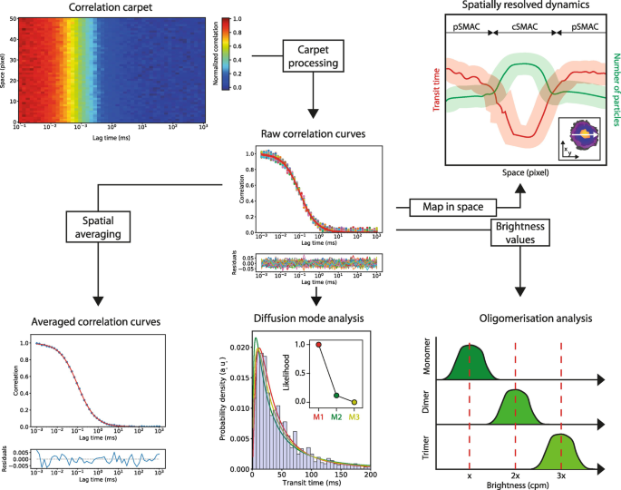

  

  Downstream analysis of sFCS data. Flowchart demonstrating four examples of downstream analysis possible with sFCS: spatial averaging to improve SNR, transit time histogram analysis to reveal diffusion modes (i.e., best fit to model M1, M2, or M3), spatially resolved mapping of fitting parameters to reveal heterogeneities in space (e.g., across an immunological synapse as shown in the inset), and brightness analysis to reveal oligomeric states

  To obtain accurate ω values, it is important to use a dye with similar spectral properties as the fluorophore of interest as this will affect the size of the excitation volume (i.e., use the same excitation line). ω can then be used to obtain the diffusion coefficient of the fluorophore of interest, facilitating comparison of diffusion data with other studies (see Note 16).

• 3. Convert the average number of particles (N) into fluorophore densities (e.g., molecules per μm²) using the same calibrated beam waist radius as for the transit time. Once ω is known, N can be normalized by observation area/volume (circular area = πω², elliptical volume = π^3/2ω³AR) to calculate fluorophore density.

• 4. Perform statistical analysis of non-averaged transit times to infer the diffusion mode of the fluorophores. This is because nanoscale hindrances in diffusion (like transient binding/trapping events or constrained diffusion) cause changes in the distribution of the transit times [47]. The diffusion mode can be inferred by determining if a free diffusion model (lognormal model) or a hindered diffusion model (e.g., double lognormal model) represents the histogram data best. Relative likelihood values can be calculated using a custom-written Python script available on GitHub (https://github.com/Faldalf/sFCS_BTS/tree/main/Scripts).

3.10 Example Data: Lck Diffusion in T Cells Is Linked to Activatory Signaling

Lck, the signal-initiating kinase of T cells, becomes recruited to signaling microclusters upon activation of the T-cell receptor (TCR) [49]. Lck is anchored to the inner leaflet of the plasma membrane via palmitoylation sites [50], resulting in slower diffusion relative to cytoplasmic proteins and making it an ideal target for analysis with sFCS. To study the effect of absence and presence of the T-cell signaling machinery on the diffusion mode of Lck, we used sFCS to measure Lck dynamics when expressed in either fibroblastic HEK293T cells (Fig. 8a-d) or a model T-cell system (leukemic Jurkat T cells, Fig. 8e-h). Cells expressing fluorescent human Lck-EGFP were incubated on glass coverslips either non-coated (HEK cells) or coated with OKT3 (strongly activating anti-CD3 antibody, Jurkat cells) and sFCS measurements were performed by acquiring intensity traces (Fig. 8b,f) followed by correlation yielding correlation carpets (Fig. 8c,g) as described in Sect. 3.8. Fitting of the correlation curves produced transit times for distribution analysis. Lck dynamics in HEK or Jurkat cells show similar median transit times (HEK cells, 25.8 ms; Jurkat cells, 22.1 ms; see Note 17). However, the maximum likelihood analysis shows that the transit time histograms from Lck in HEK cells are characteristic of freely diffusing Lck (Fig. 8d, lognormal), whereas hindered diffusion of Lck is observed in Jurkat cells on OKT3 (Fig. 8h, double lognormal). This indicates a change in bulk Lck diffusion mode from free to trapped diffusion upon activation of the TCR signaling, demonstrating how sFCS can be used to detect nanoscale interactions using diffraction-limited confocal imaging.

Fig. 8

Example sFCS data on Lck-EGFP organization in HEK 293 T cells and Jurkat T-cells on OKT3-coated coverslips. a. Fluorescence image of Lck-EGFP excited with 488 nm in HEK293T cells. b. Intensity time trace for a single sFCS carpet (sum of all pixels over acquisition time, t). c. sFCS correlation carpet for a typical measurement on Lck-EGFP in HEK293T cells. d. Transit time histogram and model selection via maximum likelihood estimation. The most likely model (relative likelihood value of 1) is the lognormal (Lognorm, indicating free diffusion). e. Confocal fluorescence image of a T-cell expressing Lck-EGFP and spreading on the coverslip (left) and transmission bright field image (right). The yellow arrow indicates a typical sFCS measurement line. f. Intensity time trace for a single sFCS acquisition of Lck-EGFP. g. Correlation carpet for a typical sFCS measurements. h. Transit time histogram and model selection via maximum likelihood estimation. The most likely model describing the diffusion of Lck-EGFP in the Jurkat T-cells on OKT3-coated glass is double lognormal (dLognorm, indicating hindered diffusion)

4 Notes

• 1. sFCS measurements can, in principle, be performed on any confocal laser scanning microscope (LSM). Perform sFCS and fluctuation measurements with high-grade, high numerical aperture (NA), chromatically corrected, water immersion objectives. For measurements at the bottom membrane of the cell (no further than a few microns above the coverslip surface), measurements with a high NA oil immersion objective might enable a better signal-to-noise ratio (SNR). The magnification of the objective determines the maximum length of the sFCS measurement.

• 2. Collect fluorescence through appropriate dichroic mirror and emission filters onto highly sensitive detectors such as single-photon avalanche diodes (SPADs) or hybrid detectors operating in photon counting mode. If you need to perform the sFCS measurements in integration mode (scaling of the intensity, gain are applied) or on a photon multiplier tube (PMT), the intensity values will not directly relate to photon counts, and you will be required to calibrate the detector gain.

• 3. pFCS measurements are conventionally used for assessing performance of the confocal system prior to performing sFCS acquisitions. pFCS requires the capability to acquire fluorescence intensity in one location (pixel) over time and can be used to calculate ACFs “on the go.” This is not a strict requirement but helps with alignment and calibration. The steps described are for a Zeiss LSM 780 with a C-Apochromat 63x 1.2 NA Korr objective for FCS and running the ZEN FCS software module but are easily transferrable to a Zeiss 880 or 980. We have also used it successfully on a Leica SP8, PicoQuant Microtime 200, and Abberior microscope. Consult your microscope facility manager or manufacturer applications support specialists on how to acquire the same information on the confocal system available to you.

• 4. See this PicoQuant Application Note (ref. [51]) for an overview of diffusion coefficients of common dyes. There is also a description of how to adjust diffusion coefficients and viscosity for measurements at different temperatures.

• 5. We recommend using the same sample holder for both the calibration dyes and the samples using multi-well chambers (e.g., MatTek dishes or ibidi multi-well slides). This is to ensure the system is calibrated for the same glass coverslip that samples are measured on.

• 6. In some commercial microscopes, the pinhole alignment needs to be performed manually by screws displacing the pinhole in x,y (e.g., Abberior, PicoQuant).

• 7. Excitation scans can provide useful information to reproduce measurements and keep an eye on microscope performance. In addition, it is advisable to measure the absolute laser power either at the back focal plane of the objective or at the objective lens using a power meter. This allows converting % of laser power to μW or W/cm² allowing to compare measurements at different microscopes as laser output (given in %) is very different between different microscopes and lasers.

• 8. As a technical FCCS control, DNA oligonucleotides labeled with two organic dyes or a tandem construct in which two FPs are linked together in the same polypeptide can be used for initial assessment and calibration of the instrumentation and materials [29]. If low cross-correlation is obtained with this in vitro control, the microscope might be misaligned or the objective might be not corrected for chromatic aberrations. Imaging fluorescent beads that fluoresce in multiple colors can be used for further troubleshooting [23]. Contact the microscope vendor or the core facility manager for further assistance if the in vitro controls and fluorescent beads show clear misalignment and aberrations.

• 9. Live cells can be challenging samples for sFCS since the effective fluorophore concentration must remain constant in the observation area over the course of the measurement period (~1 min). This means that any physical processes which drive local increases or decreases in fluorophore density (e.g., membrane undulations, large protein clusters, membrane protrusions, vesicular trafficking) contribute to a decrease in signal quality. In our experience, adherent cells are more amenable for sFCS analysis than suspensions cells due to their propensity to form flat and stable cell contacts with a homogenous protein distribution. To successfully measure suspension cells, like Jurkat T cells, additional efforts are required to prepare surfaces to which the cells can adhere without migrating. Molecules of interest can then either be labeled exogenously with antibodies or their fragments or tagged endogenously with fluorescent protein labels like mEGFP or mCherry2 [38]. In the case of the latter, sFCS measurements can only be performed on relatively dim cells, and so we recommend transient transfections (which generate a broad distribution of positive cells) over stable transductions (which tends to favor a narrow and higher expression level).

• 10. In our experience, blocking of lipid bilayers with 5% BSA can slow lateral diffusion by up to an order of magnitude. If this presents a problem, we recommend titrating BSA or comparing to unblocked bilayers. With sufficiently clean preparations of lipid/protein, blocking can be omitted, but steps must be taken to ensure the homogeneity of the sample before sFCS.

• 11. Make sure the data are acquired in photon counting mode and the raw data is saved as raw counting data. On the Zeiss 780 and 880 under “Maintain,” select System Options/Hardware, and tick “Keep raw data for photon count detectors.” If this box is not ticked, the raw data are still acquired in photon counting mode but greyscaled according to bit depth. Correlation and transit time analysis is still possible; however, brightness and photons statistics become hard to interpret.

• 12. The absolute measurement time depends on the number of lines acquired, scanning frequency and pixel dwell time. For measurements on supported lipid bilayers and molecules in solution, it is advisable to scan as fast as possible as the line time (inverse scanning frequency) determines the upper time resolution (minimum lag time) of the measurement. For slower diffusing molecules, the scanning frequency can be reduced to increase pixel dwell time and photons per pixel. This is especially helpful with dim fluorophores. This needs to be optimized for every case. Start with fastest scanning.

• 13. To extract quantitative data from the correlation curves, they need to be fitted to an appropriate model. Models describing the resulting fluctuations for various processes such as diffusion in two or three dimensions, flow, blinking and various other scenarios have been derived elsewhere [11, 17, 24]. The models are typically of the form:

  $$ G\left(\tau \right)=G(0)\dot{\textrm{c}}\left({G}_D\left(\tau \right)\dot{\textrm{c}}{G}_T\left(\tau \right)\right)+ offset $$

  (2)

  Here, G(0) refers to the amplitude which is inversely correlated to the average number of molecules in focus $G(0)\sim \frac{1}{N}$. G_D(τ) describes one or multiple diffusive terms accounting, for example, for 2D or 3D diffusion. G_T(τ) describes contributions to fluctuations through the triplet state. Notably, Eq. (2) can be extended to account for multiple diffusing species and/or triplet states. Correlation curves should be falling to 1 (or zero based on normalization). However, bleaching, drift, or duration noise can cause deviations from that and can be accounted for by including an offset. In sFCS, fluctuations due to 3D diffusion or triplet states are often lost due to the lower temporal resolution, and thus mostly a simple 2D diffusion model suffices to fit the data. However, for the calibration with the solution dye (using pFCS), the 3D model and triplet is required and given here as well:

  $$ 3\textrm{D}\ \textrm{diffusion}:{G}_{3D}\left(\tau \right)={\left(1+\left(\frac{\tau }{\tau_D}\right)\right)}^{-1}\dot{\textrm{c}}{\left(1+\frac{\tau }{A{R}^2\dot{\textrm{c}}{\tau}_D}\right)}^{\frac{1}{2}} $$

  (3)
  $$ \textrm{Triplet}\ \textrm{state}\ \textrm{contribution}:{G}_T\left(\tau \right)=1+\left(\frac{T_T}{1-{T}_T}\right)\mathit{\exp}\frac{-\tau }{\tau_T} $$

  (4)
  $$ 2\textrm{D}\textrm{diffusion}:\kern4.00em {G}_{2D}\left(\tau \right)={\left(1,+,\left(\frac{\tau }{\tau_D}\right)\right)}^{-1} $$

  (5)

  FCS fitting models can also account for sub- or super-diffusive processes by inclusion of an exponential parameter often referred to as alpha, α. Fitting alpha can account for various physical processes and thus improve data fitting. However, given the comparably low SNR in sFCS acquisitions, we suggest keeping alpha fixed to 1. In general, when fitting data, as many parameters as possible should be kept fixed. Typically, in sFCS, amplitude, transit time, and offset (if necessary) are floating parameters.

• 14. Inspect the intensity carpet or average intensity per pixel (given next to the correlation carpet in FoCuS_scan) for systematic deviations or patterns in intensity. Galvo scanners use a sinusoidal function to scan the laser beam and create the LSM image. This means that the beam scanning accelerates or decelerates at the edges of the scanned area which causes longer pixel dwell times resulting in higher intensities. In most commercial setups, this effect is corrected for. If not, spatially cropping the correlation carpet allows to remove faulty pixels from sFCS measurements.

• 15. Fitting FCS requires a general idea of the underlying process causing the intensity fluctuations. Initial parameters as well as minimum/maximum limits for the fitted value depend on what is appropriate for the physical situation. As also nomenclature of the fitting parameters can be confusing, we provide Table 1 below for guidance.

  Table 1 Fitting parameters for FCS curves. The table gives an overview of the fitting parameters commonly encountered when fitting (s)FCS data. We provide the terms by which parameters are typically referred to in the literature and their naming in FoCuS_scan. Please note that some parameters may appear multiple times if, for example, two-component diffusion has to be fitted (two transit times, two alpha values will need to be fitted, etc.). The suggested range needs to be adjusted given the experimental setting (e.g., measurements at very low concentrations << nM may exceed amplitude values of 10). We suggest using a value close to the expected parameter for initialization of the fit; otherwise use the geometric mean of the fitting range as initialization parameter

• 16. Calibration can be omitted using spatiotemporal correlation analysis. By correlating the pixels not only in time but also in space, the beam waist radius can be estimated, and the measurement can be considered self-calibrated though only yielding a single diffusion coefficient per carpet [52,53,54]. The spatiotemporal correlation approach is powerful, yet computationally expensive and not supported in FoCuS_scan.

• 17. sFCS can quickly generate large sets of data. To compare between different conditions, for example, different SLB preparations, we suggest to not compare the raw data (hundreds of data points) but to rather use the median value (or fitted μ values from the statistical analysis) to compare data from different preparations. Pooled data should be normally distributed, and standard t-test statistics can be applied.

References

Grakoui A, Bromley SK, Sumen C, et al (1999) The immunological synapse: a molecular machine controlling T cell activation. Science 285:221–227. https://doi.org/https://doi.org/10.1126/science.285.5425.221
Dustin ML (2014) The immunological synapse. Cancer. Immunol Res 2:1023–1033
Kaizuka Y, Douglass AD, Varma R, et al (2007) Mechanisms for segregating T cell receptor and adhesion molecules during immunological synapse formation in Jurkat T cells. Proc Natl Acad Sci U S A 104:20296–20301. https://doi.org/https://doi.org/10.1073/pnas.0710258105
Demetriou P, Abu-Shah E, Valvo S, et al (2020) A dynamic CD2-rich compartment at the outer edge of the immunological synapse boosts and integrates signals. Nat Immunol 21:1232–1243. https://doi.org/https://doi.org/10.1038/s41590-020-0770-x
Hartman NC, Nye JA, Groves JT (2009) Cluster size regulates protein sorting in the immunological synapse. Proc Natl Acad Sci U S A 106:12729–12734. https://doi.org/https://doi.org/10.1073/pnas.0902621106
Comrie WA, Burkhardt JK (2016) Action and traction: cytoskeletal control of receptor triggering at the immunological synapse. Front Immunol 7:68
Phillips R, Milo R (2009) A feeling for the numbers in biology. Proc Natl Acad Sci U S A 106:21465–21471
Waithe D, Schneider F, Chojnacki J, et al (2018) Optimized processing and analysis of conventional confocal microscopy generated scanning FCS data. Methods 140–141:62–73. https://doi.org/https://doi.org/10.1016/j.ymeth.2017.09.010
Sezgin E, Schneider F, Galiani S, et al (2019) Measuring nanoscale diffusion dynamics in cellular membranes with super-resolution STED–FCS. Nat Protoc 14:1054–1083. https://doi.org/https://doi.org/10.1038/s41596-019-0127-9
Magde D, Elson E, Webb WW (1972) Thermodynamic fluctuations in a reacting system measurement by fluorescence correlation spectroscopy. Phys Rev Lett 29:705–708. https://doi.org/https://doi.org/10.1103/PhysRevLett.29.705
Magde D, Elson EL, Webb WW (1974) Fluorescence correlation spectroscopy. II An experimental realization Biopolymers 13:29–61. https://doi.org/https://doi.org/10.1002/bip.1974.360130103
Ehrenberg M, Rigler R (1974) Rotational brownian motion and fluorescence intensify fluctuations. Chem Phys 4:390–401. https://doi.org/https://doi.org/10.1016/0301-0104(74)85005-6
Kim SA, Heinze KG, Schwille P (2007) Fluorescence correlation spectroscopy in living cells. Nat Methods 4:963–973. https://doi.org/https://doi.org/10.1038/nmeth1104
Bacia K, Schwille P (2007) Practical guidelines for dual-color fluorescence cross-correlation spectroscopy. Nat Protoc 2:2842–2856. https://doi.org/https://doi.org/10.1038/nprot.2007.410
Digman MA, Gratton E (2011) Lessons in fluctuation correlation spectroscopy. Annu Rev Phys Chem 62:645–668. https://doi.org/https://doi.org/10.1146/annurev-physchem-032210-103424
Schneider F, Colin-York H, Fritzsche M (2021) Quantitative bio-imaging tools to dissect the interplay of membrane and cytoskeletal actin dynamics in immune cells. Front Immunol 11:1–13
Lackowicz J (2006) Principles of fluorescence spectroscopy, Third. Springer US, Boston, MA
Koppel DE, Axelrod D, Schlessinger J, et al (1976) Dynamics of fluorescence marker concentration as a probe of mobility. Biophys J 16:1315–1329. https://doi.org/https://doi.org/10.1016/S0006-3495(76)85776-1
Ruan Q, Cheng MA, Levi M, et al (2004) Spatial-temporal studies of membrane dynamics: scanning fluorescence correlation spectroscopy (SFCS). Biophys J 87:1260–1267. https://doi.org/https://doi.org/10.1529/biophysj.103.036483
Ries J, Yu SR, Burkhardt M, et al (2009) Modular scanning FCS quantifies receptor-ligand interactions in living multicellular organisms. Nat Methods 6:643–645. https://doi.org/https://doi.org/10.1038/nmeth.1355
Gunther G, Jameson DM, Aguilar J, Sánchez SA (2018) Scanning fluorescence correlation spectroscopy comes full circle. Methods 140–141:52–61
Priest DG, Solano A, Lou J, Hinde E (2019) Fluorescence fluctuation spectroscopy: an invaluable microscopy tool for uncovering the biophysical rules for navigating the nuclear landscape. Biochem Soc Trans 47:1117–1129
Dunsing V, Petrich A, Chiantia S (2021) Spectral detection enables multi-color fluorescence fluctuation spectroscopy studies in living cells. Biophys J 120:356a. https://doi.org/https://doi.org/10.1016/j.bpj.2020.11.2206
Elson EL (2011) Fluorescence correlation spectroscopy: past, present, future. Biophys J 101:2855–2870
Hink MA (2014) Fluorescence correlation spectroscopy. Methods Mol Biol 1251:135–150. https://doi.org/https://doi.org/10.1007/978-1-4939-2080-8_8
Dunsing V, Mayer M, Liebsch F, et al (2017) Direct evidence of amyloid precursor-like protein 1 trans interactions in cell-cell adhesion platforms investigated via fluorescence fluctuation spectroscopy. Mol Biol Cell 28:3609–3620. https://doi.org/https://doi.org/10.1091/mbc.E17-07-0459
Dörlich RM, Chen Q, Niklas Hedde P, et al (2015) Dual-color dual-focus line-scanning FCS for quantitative analysis of receptor-ligand interactions in living specimens. Sci Rep 5:10149. https://doi.org/https://doi.org/10.1038/srep10149
Krieger JW, Singh AP, Bag N, et al (2015) Imaging fluorescence (cross-) correlation spectroscopy in live cells and organisms. Nat Protoc 10:1948–1974. https://doi.org/https://doi.org/10.1038/nprot.2015.100
Lee W, Lee YI, Lee J, et al (2010) Cross-talk-free dual-color fluorescence cross-correlation spectroscopy for the study of enzyme activity. Anal Chem 82:1401–1410. https://doi.org/https://doi.org/10.1021/ac9024768
Valvo S, Mayya V, Seraia E, et al (2017) Comprehensive analysis of immunological synapse phenotypes using supported lipid bilayers. Methods Mol Biol 1584:423–441. https://doi.org/https://doi.org/10.1007/978-1-4939-6881-7_26
Dustin ML, Baldari CT (2017) The immune synapse: past, present, and future. In: Methods in molecular biology. Humana Press Inc., pp 1–5
Dustin ML, Starr T, Varma R, Thomas VK (2007) Supported planar bilayers for study of the immunological synapse. Curr Protoc Immunol Chapter 18:18.13.1–18.13.35. https://doi.org/https://doi.org/10.1002/0471142735.im1813s76
Schneider F, Hernandez-Varas P, Christoffer Lagerholm B, et al (2020) High photon count rates improve the quality of super-resolution fluorescence fluctuation spectroscopy. J Phys D Appl Phys 53:164003. https://doi.org/https://doi.org/10.1088/1361-6463/ab6cca
Enderlein J, Gregor I, Patra D, Fitter J (2005) Art and artefacts of fluorescence correlation spectroscopy. Curr Pharm Biotechnol 5:155–161. https://doi.org/https://doi.org/10.2174/1389201043377020
Gregor I, Patra D, Enderlein J (2005) Optical saturation in fluorescence correlation spectroscopy under continuous-wave and pulsed excitation. ChemPhysChem 6:164–170. https://doi.org/https://doi.org/10.1002/cphc.200400319
Digman MA, Dalal R, Horwitz AF, Gratton E (2008) Mapping the number of molecules and brightness in the laser scanning microscope. Biophys J 94:2320–2332. https://doi.org/https://doi.org/10.1529/biophysj.107.114645
Dunsing V, Chiantia S (2018) A fluorescence fluctuation spectroscopy assay of protein-protein interactions at cell-cell contacts. J Vis Exp 2018:1–16. https://doi.org/https://doi.org/10.3791/58582
Dunsing V, Luckner M, Zühlke B, et al (2018) Optimal fluorescent protein tags for quantifying protein oligomerization in living cells. Sci Rep 8:1–12. https://doi.org/https://doi.org/10.1038/s41598-018-28858-0
Schneider F, Waithe D, Clausen MP, et al (2017) Diffusion of lipids and GPI-anchored proteins in actin-free plasma membrane vesicles measured by STED-FCS. Mol Biol Cell 28:1507–1518. https://doi.org/https://doi.org/10.1091/mbc.E16-07-0536
Faizi HA, Tsui A, Dimova R, Vlahovska PM (2022) Bending rigidity, capacitance, and shear viscosity of Giant vesicle membranes prepared by spontaneous swelling, Electroformation, gel-assisted, and phase transfer methods: a comparative study. Langmuir 38:10548–10557. https://doi.org/https://doi.org/10.1021/ACS.LANGMUIR.2C01402
Montes LR, Ahyayauch H, Ibarguren M, et al (2010) Electroformation of giant unilamellar vesicles from native membranes and organic lipid mixtures for the study of lipid domains under physiological ionic-strength conditions. Methods Mol Biol 606:105–114. https://doi.org/https://doi.org/10.1007/978-1-60761-447-0_9
Santos AM, Ponjavic A, Fritzsche M et al (2018) Capturing resting T cells: the perils of PLL. Nat Immunol 19:203–205
Dam T, Junghans V, Humphrey J, et al (2021) Calcium signaling in T cells is induced by binding to nickel-chelating lipids in supported lipid bilayers. Front Physiol 11:1878. https://doi.org/https://doi.org/10.3389/fphys.2020.613367
Waithe D (2021) Open-source browser-based software simplifies fluorescence correlation spectroscopy data analysis. Nat Photonics 15:790–791
Müller P, Schwille P, Weidemann T (2014) PyCorrFit-generic data evaluation for fluorescence correlation spectroscopy. Bioinformatics 30:2532–2533. https://doi.org/https://doi.org/10.1093/bioinformatics/btu328
Rossow MJ, Sasaki JM, Digman MA, Gratton E (2010) Raster image correlation spectroscopy in live cells. Nat Protoc 5:1761–1774. https://doi.org/https://doi.org/10.1038/nprot.2010.122
Schneider F, Waithe D, Lagerholm BC, et al (2018) Statistical analysis of scanning fluorescence correlation spectroscopy data differentiates free from hindered diffusion. ACS Nano 12:8540–8546. https://doi.org/https://doi.org/10.1021/acsnano.8b04080
Mørch AM, Schneider F, Jenkins E, et al (2022) The kinase occupancy of T-cell coreceptors reconsidered bioRxiv 2022.08.01.502332. https://doi.org/10.1101/2022.08.01.502332
Smith-Garvin JE, Koretzky GA, Jordan MS (2009) T cell activation. Annu Rev Immunol 27:591–619. https://doi.org/https://doi.org/10.1146/annurev.immunol.021908.132706.T
Kabouridis PS, Magee AI, Ley SC (1997) S-acylation of LCK protein tyrosine kinase is essential for its signalling function in T lymphocytes. EMBO J 16:4983–4998. https://doi.org/https://doi.org/10.1093/emboj/16.16.4983
Kapusta P (PicoQuant) (2010) Absolute Diffusion Coefficients: Compilation of Reference Data for FCS Calibration
Benda A, Ma Y, Gaus K (2015) Self-calibrated line-scan STED-FCS to quantify lipid dynamics in model and cell membranes. Biophys J 108:596–609. https://doi.org/https://doi.org/10.1016/j.bpj.2014.12.007
Maraspini R, Beutel O, Honigmann A (2018) Circle scanning STED fluorescence correlation spectroscopy to quantify membrane dynamics and compartmentalization. Methods 140–141:188–197. https://doi.org/https://doi.org/10.1016/j.ymeth.2017.12.005
Ries J, Chiantia S, Schwille P (2009) Accurate determination of membrane dynamics with line-scan FCS. Biophys J 96:1999–2008. https://doi.org/https://doi.org/10.1016/j.bpj.2008.12.3888
Cairo CW, Das R, Albohy A, et al (2010) Dynamic regulation of CD45 lateral mobility by the spectrin-ankyrin cytoskeleton of T cells. J Biol Chem 285:11392–11401. https://doi.org/https://doi.org/10.1074/jbc.M109.075648
Zhu DM, Dustin ML, Cairo CW, Golan DE (2007) Analysis of two-dimensional dissociation constant of laterally mobile cell adhesion molecules. Biophys J 92:1022–1034. https://doi.org/https://doi.org/10.1529/biophysj.106.089649
Cairo CW, Mirchev R, Golan DEE (2006) Cytoskeletal regulation couples LFA-1 conformational changes to receptor lateral mobility and clustering. Immunity 25:297–308. https://doi.org/https://doi.org/10.1016/j.immuni.2006.06.012
D’Oro U, Munitic I, Chacko G, et al (2002) Regulation of constitutive TCR internalization by the ζ-chain. J Immunol 169:6269–6278. https://doi.org/https://doi.org/10.4049/jimmunol.169.11.6269
Hilzenrat G, Pandžić E, Yang Z, et al (2020) Conformational states control Lck switching between free and confined diffusion modes in T cells. Biophys J 118:1489–1501. https://doi.org/https://doi.org/10.1016/j.bpj.2020.01.041
Yi J, Wu XS, Crites T, Hammer JA (2012) Actin retrograde flow and actomyosin II arc contraction drive receptor cluster dynamics at the immunological synapse in Jurkat T cells. Mol Biol Cell 23:834–852. https://doi.org/https://doi.org/10.1091/mbc.E11-08-0731
Varma R, Campi G, Yokosuka T, et al (2006) T cell receptor-proximal signals are sustained in peripheral microclusters and terminated in the central supramolecular activation cluster. Immunity 25:117–127. https://doi.org/https://doi.org/10.1016/j.immuni.2006.04.010
Acknowledgments
AMM acknowledges funding from the Wellcome Trust PhD Studentship in Science (108869/Z/15/Z). FS is grateful for the long-term postdoctoral fellowship support from EMBO (EMBO ALTF 849-2020) and HFSP (LT000404/2021-L). FS and AMM thank their supervisors Scott E. Fraser and Michael L. Dustin for the freedom to pursue this project. The authors are grateful for the proof-reading and comments by Jiarui Wang and João Ferreira Fernandes. Finally, the authors thank Dr. Dominic Waithe for the development of and the continuous effort to support the open-source FoCuS_scan software package.
Authors Contributions
AMM and FS wrote the manuscript and prepared the figures. The final text has been approved by both authors.
Author information
Authors and Affiliations
Corresponding author
Editor information
Editors and Affiliations
Rights and permissions
Open Access This chapter is licensed under the terms of the Creative Commons Attribution 4.0 International License (http://creativecommons.org/licenses/by/4.0/), which permits use, sharing, adaptation, distribution and reproduction in any medium or format, as long as you give appropriate credit to the original author(s) and the source, provide a link to the Creative Commons license and indicate if changes were made.
The images or other third party material in this chapter are included in the chapter's Creative Commons license, unless indicated otherwise in a credit line to the material. If material is not included in the chapter's Creative Commons license and your intended use is not permitted by statutory regulation or exceeds the permitted use, you will need to obtain permission directly from the copyright holder.
Copyright information
© 2023 The Author(s), under exclusive license to Springer Science+Business Media, LLC, part of Springer Nature
About this protocol
Cite this protocol
Mørch, A.M., Schneider, F. (2023). Investigating Diffusion Dynamics and Interactions with Scanning Fluorescence Correlation Spectroscopy (sFCS). In: Baldari, C.T., Dustin, M.L. (eds) The Immune Synapse. Methods in Molecular Biology, vol 2654. Humana, New York, NY. https://doi.org/10.1007/978-1-0716-3135-5_5
Download citation
DOI: https://doi.org/10.1007/978-1-0716-3135-5_5
Published:
Publisher Name: Humana, New York, NY
Print ISBN: 978-1-0716-3134-8
Online ISBN: 978-1-0716-3135-5
eBook Packages: Springer Protocols