
Abstract
Reduction of attributes in an information system (IS) is a basic step for IS analysis. The original rough set model of Pawlak depends on an equivalence relation which is strongly constraints. This paper aims to use similarity classes and similarity degrees to obtain a reduction of IS and indicate an approach by using an example from biochemistry to get a quantitative structure activity relationship (QSAR). Moreover, signs of each attribute and degrees of memberships are computed to give a decision by using the degree of similarity. The suggested approach gives an increase in decision-making and decision accuracy.
Introduction and preliminaries
The rough set theory of Pawlak [1] is a mathematical tool to analyze the uncertain data. Pawlak classified data to a set of classes, and each class consists of objects [2]. This classification depends on an equivalence relation, and so all objects in the same class have the same importance, but this is not true in real life for all uncertain data. The notion of membership was studied in the view point of topological spaces in [3] and [4] via a general binary relation. This membership was extended from the original rough membership function [5]. Allam et al. [6] and Salama [7] gave a new approach for basic rough set concepts. They obtained some topological structures from rough sets. In [8], Yao et al. discussed the issue of classes overlapping in rough sets and they introduced a membership of an object to a class. The approximations is used to calculate the accuracy as in [9]. Several studies such as a chemical topology [10] have focused on the stability of structure bonds in proteins. Also, similarity on rough sets is one of these studies which interests in the protein energy of unfolding. Similarity based on rough sets was discussed in [11] and [12]. In 2017, Elshenawy et al. [13] studied the similarity of data via a weighted membership. Walczak and Massart [14] classified the data by giving range chosen. They used lower and upper approximations to calculate the accuracy. In this case, the intersection of all reducts gives the core of attributes. The topology on X generated by R is a knowledge base for X, and indication of symptoms for a fixed disease can be seen through the topology [15]. Different notions of a membership function based on rough sets were introduced and studied in [16], [17], and [18]. A QSAR [19] constructs a mathematical model interconnected in its biological activity a set of structural descriptors of a set of chemical compounds. The main purpose of this paper is to study the reduction based on similarity. We give a comparison between a reduction by similarity and some other types of reduction with some different examples. An application on QSAR of AAs will be studied. We introduce an algorithm to reduce a membership function and illustrate it graphically. Some properties of relations and membership functions will be investigated. A new method is introduced to study the correlation between attributes and a decision through a similarity relation.
Definition 1
[1] The IS or approximation space is a system (U,A,f) where U is the universe of finite set of objects and A is a set of attributes which is featured or variables. Each a∈A defines an information function fa:U→Va, where Va is the set of all values of a, say the domain of attribute a.
Definition 2
[5] For every B⊆A, the indiscernibility relation on B, denoted by Ind(B), is defined to be two objects xi,xj∈U which are indiscernible by the sets B if b(xi)=b(xj) for every b∈B. Ind(B) is the smallest indiscernible groups of objects and so the equivalence class of Ind(B) called elementary set in B. [xi] will denote to the equivalence class of object xi in the relation Ind(B).
Definition 3
[5] For every B⊆A, a membership function of an object xi∈U with respect to B is given by \(\mu _{B}(x_{i})= \frac {|[x_{i}]\cap B|}{|[x_{i}]|}\), where |[xi]| is the cardinality the class [xi], in other words, the number of objects contained in [xi].
The IS is represented in Table 1 with a set of attributes A={p,q,r,s} and a set of objects U={a,b,c,d,e}. We study the effect of attributes on decision, in other words, the correlation between attributes and the decision in the following statements.
Original Pawlak method
In Table 1, we compare between attributes of objects. There is no similarity between attributes of objects. So, we have the class of objects C={{a},{b},{c},{d},{e}} and two sets of decisions D1={a,d,e} and D2={b,c}. The Pawlak membership is given by \(\mu _{A}(x) = \frac {|[x]\cap A |}{|[x]|}\), for any object x and A⊆U. Therefore:
This means any object correlates with the decision only by 0 and 1.
Pawlak method with coding
The IS in Table 1 can be coded by choosing intervals as in Table 2. The IS with coding is given by Table 3. The class of objects in Table 3 is C={{a},{b,c},{d},{e}}. Objects correlate with decisions D1 and D2 by:
This means that any object correlates with the decision only by 0, \(\frac {1}{2}\) and 1.
Similarity without degree
The similarity matrix between objects in Table 3 is given by Table 4. A binary relation R on U is defined by xRy if and only if \(\mu (x, y)\leq \frac {1}{4}\). Then, the class of objects is C={U,{a,b,d},{a,c,d}},{a,d,e}. The correlation of objects with respect to decisions D1 and D2 is given by\(\mu _{D_{1}}(a)= \frac {|U\cap \{a, b, d\}\cap \{a, c, d\}\}\cap \{a, d, e\}|}{| D_{1}|}= \frac {|\{a, d\}|}{| D_{1}|}= \frac {2}{3}\), \(\mu _{D_{1}}(b)= 1\), \(\mu _{D_{1}}(c)= 1\), \(\mu _{D_{1}}(d)= \frac {2}{3}\), \(\mu _{D_{1}}(e)= 1\). Also, \(\mu _{D_{2}}(a)= 1\), \(\mu _{D_{2}}(b)= \frac {3}{2}\), \(\mu _{D_{2}}(c)= \frac {3}{2}\), \(\mu _{D_{2}}(d)= 1\) and \(\mu _{D_{2}}(e)= \frac {3}{2}\).
Uncertain QSAR information system
The basic form of Pawlak depends on equivalence relation. This expands the application circle for objects and decision rules. Because if we apply Pawlak rules for some ISs, it is not possible to have equal attributes for two different attributes. So as in the following problem, that we are giving a method of solving depends on a similarity relation.
Problem A modeling of the energy of unfolding of a protein (tryptophane synthase an alpha unit of the bacteriophage T4 lysozome), where 19 coded amino acids (AAs) were each introduced into position 49 [20]. The AAs are described in terms of seven attributes: a1= PIE and a2= PIF (two measures of the side chain lipophilicity), a3= DGR =ΔG of transfer from the protein interior with water, a4= SAC = surface area, a5= MR = molecular refractivity, a6= LAM = the side chain polarity, and a7= Vol = molecular volume. In [14], the authors used the form of Pawlak [1] to make decision rules. The IS of quantitative attributes {a1,a2,a3,a4,a5,a6,a7} and a decision attribute {d} can be represented by Table 5. The condition attributes are coded into four qualitative terms, such as very low, low, high, and very high, whereas the decision attributes is coded into three qualitative terms, such as low, medium, and high. The qualitative terms of all attributes are coded by integer numbers. The problem is to illustrate that there are some objects that coded with medium energy of unfolding in [14] in respect of an attribute would be for the high energy of unfold.
Algorithm
Step 1: Construct a similarity matrix for each attribute a by Ma=[wij] which will be 19×19 matrix, 7 is the number of attributes, i∈{1,2,3,⋯,19} will denote to the row of matrix, and j∈{1,2,3,⋯,19} will denote to the column of the matrix.
Step 2: Calculate the similarity degree of attributes through a definite relation, say R, on the our IS which will be denoted by QSAR IS=(U,A), where U={x1,x2,x3,x4,x5,x6,x7,x8,x9,x10,x11,x12,x13,x14,x15,x16,x17,x18,x19} and A={a1,a2,a3,a4,a5,a6,a7}, the set of attributes. So, xiRxj if and only if xi is similar to xj. The degree of similarity or similarity measure between xi and xj is denoted by \(\text {deg}_{a}(x_{i}, x_{j})= d_{ij}= 1- \frac {|a(x_{i})- a(x_{j})|}{|a_{\text {max}}-a_{\text {min}}|}\), where amax and amin denote the minimum and maximum values of attribute a, respectively. It is clear that R is reflexive and symmetric.
Step 3: Classify the data deduced from step 2 via xiR={xj(dij):xiRxj}. The value d will be chosen by an expert. Then, there are two cases dij>d and dij<d.
Step 4: Define a membership function of every object for the similarity matrix in step 3 as follows: For any arbitrary element xkR=Ck∈U/R and for y∈Ck, the membership function of y with respect to any subset X of U, \(\mu ^{C_{k}}_{X}(y)= \frac {\sum \limits _{x\in C_{k}\cap X} d_{ij}}{\sum \limits _{x\in C_{k}}d_{ij}}\), where k∈{1,2,⋯,19}. If Ck∩X=ϕ, then \(\mu ^{C_{k}}_{X}(y)= 0\).
Step 5: Present functions of the least, most extreme, and normal weighted participation for every y by:
Step 6: Choose a set X⊂U. Evaluate the rough membership μ for each object z by determining the \(A= \bigcap \limits _{z\in C_{k}} C_{k}\) and calculate \(\mu = \frac {|A\cap X|}{|A|}\), for every object.
Step 7: Determine a maximum rough membership μ from the last column of each classification.
Now, we apply the algorithm on the problem of QSAR.
- (1)
Similarity matrix for an attribute a1. Since a1(max)=1.85 and a1(min)=−0.77, then, a1(max)−a1(min)=2.62, then we have the matrix \(M_{x_{1}}\). We have:
$$ M_{a_{1}}= \left[{\begin{array}{ccccccccccccccccccc} 1&0.7&0.7&1.0&0.9 & 0.7 & 0.9 &1.0 &0.9 &0.6 &0.6 &0.7 & 0.5& 0.9 &0.9 &1.0 &0.4 &0.7 &0.8\\ 0.7 & 1& 0.9 & 0.6& 0.9 & 1.0 & 0.8 &0.8 &0.4 &0.3 &0.9 &0.9 & 0.5& 0.2 &0.7 &0.8 &0.7 &0.5 &0.5 \\ 0.7 & 0.9& 1 & 0.6& 0.8 & 0.9 & 0.8 &0.7 &0.3 &0.3 &0.9 &0.4 & 0.2& 0.6 &0.8 &0.7 &0.1 &0.4 &0.5 \\ 1.0 & 0.6& 0.6 & 1& 0.8 & 0.6 & 0.8 &0.9 &0.7 &0.7 &0.5 &0.8 & 0.6& 0.9 &0.8 &0.9 &0.5 &0.8 &0.8 \\ 0.9 & 0.9& 0.8 & 0.8& 1 & 0.8 & 0.9 &0.9 &0.5 &0.5 &0.7 &0.6 & 0.4& 0.8 &0.9 &0.9 &0.2 &0.6 &0.4 \\ 0.7 & 1.0& 0.9 & 0.6& 0.8 & 1 & 0.8 &0.7 &0.3 &0.3 &0.9 &0.5 & 0.2& 0.7 &0.8 &0.7 &0.1 &0.5 &0.5 \\ 0.9 & 0.8& 0.8 & 0.8& 0.9 & 0.8 & 1 &0.9 &0.5 &0.5 &0.7 &0.7 & 0.4& 0.8 &1.0 &0.9 &0.3 &0.7 &0.7 \\ 1.0 & 0.8& 0.7 & 0.9& 0.9 & 0.7 & 0.9 &1 &0.6 &0.6 &0.6 &0.7 & 0.5& 0.9 &0.9 &1.0 &0.3 &0.7 &0.8 \\ 0.9 & 0.4& 0.3 & 0.7& 0.5 & 0.3 & 0.5 &0.6 &1 &0.9 &0.2 &0.9 & 0.9& 0.7 &0.5 &0.6 &0.7 &0.9 &0.8 \\ 0.6 & 0.3& 0.3 & 0.7& 0.5 & 0.3 & 0.5 &0.6 &0.9 &1 &0.2 &0.8 & 0.9& 0.7 &0.5 &0.6 &0.8 &0.8 &0.8 \\ 0.6 & 0.9& 0.9 & 0.5& 0.7 & 0.9 & 0.7 &0.6 &0.2 &0.2 &1 &0.4 & 0.1& 0.6 &0.4 &0.6 & 0.0 &0.4 &0.4 \\ 0.7 & 0.9& 0.4 & 0.8& 0.6 & 0.5 & 0.7 &0.7 &0.9 &0.8 &0.7 &1 & 0.7& 0.8 &0.7 &0.7 &0.6 &1.0 &0.9 \\ 0.5 & 0.5& 0.2 & 0.6& 0.4 & 0.2 & 0.4 &0.5 &0.9 &0.9 &0.1 &0.7 & 1& 0.5 &0.4 &0.5 &0.9 &0.7 &0.7 \\ 0.9 & 0.2& 0.6 & 0.9& 0.8 & 0.7 & 0.8 &0.9 &0.7 &0.7 &0.6 &0.8 & 0.5& 1 &0.8 &0.9 &0.4 &0.8 &0.9 \\ 0.9 & 0.7& 0.8 & 0.8& 0.9 & 0.8 & 1.0 &0.9 &0.5 &0.5 &0.7 &0.7 & 0.4& 0.8 &1 &0.9 &0.3 &0.7 &0.7 \\ 1.0 & 0.8& 0.7 & 0.9& 0.9 & 0.7 & 0.9 &1.0 &0.6 &0.6 &0.6 &0.7 & 0.5& 0.9 &0.9 &1 &0.3 &0.7 &0.8 \\ 0.4 & 0.7& 0.1 & 0.5& 0.2 & 0.1 & 0.3 &0.3 &0.7 &0.8 &0.0 &0.6 & 0.9& 0.4 &0.3 &0.3 &1 &0.6 &0.6 \\ 0.7 & 0.5& 0.4 & 0.8& 0.6 & 0.5 & 0.7 &0.7 &0.9 &0.8 &0.4 &1.0 & 0.7& 0.8 &0.7 &0.7 &0.6 &1 &0.9 \\ 0.8 & 0.5& 0.5 & 0.8& 0.7 & 0.5 & 0.7 &0.8 &0.8 &0.8 &0.4 &0.9 & 0.7& 0.9 &0.7 &0.8 &0.6 &0.9 &1 \end{array}} \right] $$ - (2)
Take d=0.7, we have the similarity classes.
$$\begin{aligned} C_{1}&= x_{1}R= \{x_{1}(1), x_{4}(1.0), x_{5}(0.9), x_{7}(0,9), x_{8}(1.0), x_{9}(0.9), x_{14}(0.9), x_{15}(0.9), x_{16}(1.0), x_{19}(0.8)\};\\ C_{2}&= x_{2}R= \{ x_{2}(1), x_{3}(0.9), x_{5}(0.9), x_{6}(1.0), x_{7}(0.8), x_{8}(0.8), x_{11}(0.9), x_{12}(0.9), x_{16}(0.8)\};\\ C_{3}&= x_{3}R= \{ x_{2}(0.9), x_{3}(1), x_{5}(0.8), x_{6}(0.9), x_{7}(0.8), x_{11}(0.9), x_{15}(0.8) \};\\ C_{4}&= x_{4}R= \{ x_{1}(1.0), x_{4}(1), x_{5}(0.8), x_{7}(0.8), x_{8}(0.9), x_{12}(0.8), x_{14}(0.9), x_{15}(0.8), x_{16}(0.9), x_{18}(0.8), x_{19}(0.8)\};\\ C_{5}&= x_{5}R= \{ x_{1}(0.9), x_{2}(0.9), x_{3}(0.8), x_{4}(0.8), x_{5}(1), x_{6}(0.8), x_{7}(0.9), x_{8}(0.9),x_{14}(0.8), x_{15}(0.9), x_{16}(0.9) \};\\ C_{6}&= x_{6}R= \{ x_{2}(1.0), x_{3}(0.9), x_{5}(0.8), x_{6}(1), x_{7}(0.8), x_{11}(0.9), x_{15}(0.8) \};\\ C_{7}&= x_{7}R= \{ x_{1}(0.9), x_{2}(0.8), x_{3}(0.8), x_{4}(0.8), x_{5}(0.9), x_{6}(0.8), x_{7}(1), x_{8}(0.9),x_{14}(0.8), x_{15}(1.0), x_{16}(0.9) \};\\ C_{8}&= x_{8}R= \{ x_{1}(1.0), x_{2}(0.8), x_{4}(0.9), x_{5}(0.9), x_{7}(0.9), x_{8}(1), x_{14}(0.9), x_{15}(0.9),x_{16}(1.0), x_{19}(0.8) \};\\ C_{9}&= x_{9}R= \{ x_{1}(0.9), x_{9}(1), x_{10}(0.9), x_{12}(0.9), x_{13}(0.9), x_{18}(0.9), x_{19}(0.8) \};\\ C_{10}&= x_{10}R= \{ x_{9}(0.9), x_{10}(1), x_{12}(0.8), x_{13}(0.9), x_{17}(0.8), x_{18}(0.8), x_{19}(0.8) \};\\ C_{11}&= x_{11}R= \{ x_{2}(0.9), x_{3}(0.9), x_{6}(0.9), x_{11}(1) \};\\ C_{12}&= x_{12}R= \{ x_{2}(0.9), x_{4}(0.8), x_{9}(0.9), x_{10}(0.8), x_{12}(1), x_{14}(0.8), x_{18}(1.0), x_{19}(0.9)\};\\ C_{13}&= x_{13}R= \{ x_{9}(0.9), x_{10}(0.9), x_{13}(1), x_{17}(0.9)\};\\ C_{14}&= x_{14}R= \{ x_{1}(0.9), x_{4}(0.9), x_{5}(0.8), x_{7}(0.8), x_{8}(0.9), x_{12}(0.8), x_{14}(1), x_{15}(0.8),x_{16}(0.9), x_{18}(0.8), x_{19}(0.9)\};\\ C_{15}&= x_{15}R= \{ x_{1}(0.9), x_{3}(0.8), x_{4}(0.8), x_{5}(0.9), x_{6}(0.8), x_{7}(1.0), x_{8}(0.9), x_{14}(0.8),x_{15}(1), x_{16}(0.9) \};\\ C_{16}&= x_{16}R= \{ x_{1}(1.0), x_{2}(0.8), x_{4}(0.9), x_{5}(0.9), x_{7}(0.9), x_{8}(1.0), x_{14}(0.9), x_{15}(0.9),x_{16}(1), x_{19}(0.8) \};\\ C_{17}&= x_{17}R= \{ x_{10}(0.8), x_{13}(0.9), x_{17}(1)\};\\ C_{18}&= x_{18}R= \{ x_{4}(0.8), x_{9}(0.9), x_{10}(0.8), x_{12}(1.0), x_{14}(0.8), x_{18}(1), x_{19}(0.9)\};\\ C_{19}&= x_{19}R= \{ x_{1}(0.8), x_{4}(0.8), x_{8}(0.8), x_{9}(0.8), x_{10}(0.8), x_{12}(0.9), x_{14}(0.9), x_{16}(0.8), x_{18}(0.9), x_{19}(1) \}. \end{aligned} $$ - (3)
We choose some various sets and compare the membership classification through the following two cases.
Case 1: Let X={x9,x10,x12}. Then, we have:
$$\begin{array}{ccccc} \mu^{C_{1}}_{X}(x_{1})= 0.10 &\mu^{C_{2}}_{X}(x_{2})= 0.11 &\mu^{C_{2}}_{X}(x_{3})= 0.11 &\mu^{C_{1}}_{X}(x_{4})= 0.10 &\mu^{C_{1}}_{X}(x_{5})= 0.10\\ \mu^{C_{4}}_{X}(x_{1})= 0.08 &\mu^{C_{3}}_{X}(x_{2})= 0.0 &\mu^{C_{3}}_{X}(x_{3})= 0.0 &\mu^{C_{4}}_{X}(x_{4})= 0.08 &\mu^{C_{2}}_{X}(x_{5})= 0.11\\ \mu^{C_{5}}_{X}(x_{1})= 0.0 &\mu^{C_{5}}_{X}(x_{2})= 0.0 &\mu^{C_{5}}_{X}(x_{3})= 0.0 &\mu^{C_{5}}_{X}(x_{4})= 0.0 &\mu^{C_{3}}_{X}(x_{5})= 0.0\\ \mu^{C_{7}}_{X}(x_{1})= 0.0 &\mu^{C_{6}}_{X}(x_{2})= 0.0 &\mu^{C_{6}}_{X}(x_{3})= 0.0 &\mu^{C_{7}}_{X}(x_{4})= 0.0 &\mu^{C_{4}}_{X}(x_{5})= 0.08\\ \mu^{C_{8}}_{X}(x_{1})= 0.0 &\mu^{C_{7}}_{X}(x_{2})= 0.0 &\mu^{C_{7}}_{X}(x_{3})= 0.0 &\mu^{C_{8}}_{X}(x_{4})= 0.0 &\mu^{C_{5}}_{X}(x_{5})= 0.0\\ \mu^{C_{9}}_{X}(x_{1})= 0.44 &\mu^{C_{8}}_{X}(x_{2})= 0.0 &\mu^{C_{11}}_{X}(x_{3})= 0.0 &\mu^{C_{12}}_{X}(x_{4})= 0.13 &\mu^{C_{6}}_{X}(x_{5})= 0.38\\ \mu^{C_{14}}_{X}(x_{1})= 0.08 &\mu^{C_{11}}_{X}(x_{2})= 0.0 &\mu^{C_{15}}_{X}(x_{3})= 0.0 &\mu^{C_{14}}_{X}(x_{4})= 0.08 &\mu^{C_{7}}_{X}(x_{5})= 0.0 \\ \mu^{C_{15}}_{X}(x_{1})= 0.0 &\mu^{C_{12}}_{X}(x_{2})= 0.38 &&\mu^{C_{15}}_{X}(x_{4})= 0.0 &\mu^{C_{8}}_{X}(x_{5})= 0.0\\ \mu^{C_{16}}_{X}(x_{1})= 0.0 &\mu^{C_{16}}_{X}(x_{2})= 0.0 &&\mu^{C_{16}}_{X}(x_{4})= 0.0 &\mu^{C_{14}}_{X}(x_{5})= 0.08\\ \mu^{C_{19}}_{X}(x_{1})= 0.30 &&&\mu^{C_{18}}_{X}(x_{4})= 0.44 &\mu^{C_{15}}_{X}(x_{5})= 0.0\\ &&& \mu^{C_{19}}_{X}(x_{4})= 0.30 & \mu^{C_{16}}_{X}(x_{5})= 0.0 \end{array}$$and
$$\begin{array}{cccccc} \mu^{C_{2}}_{X}(x_{6})= 0.11 &\mu^{C_{1}}_{X}(x_{7})= 0.10 &\mu^{C_{1}}_{X}(x_{8})= 0.10 &\mu^{C_{1}}_{X}(x_{9})= 0.10 &\mu^{C_{9}}_{X}(x_{10})= 0.44\\ \mu^{C_{3}}_{X}(x_{6})= 0.0 &\mu^{C_{2}}_{X}(x_{7})= 0.11 &\mu^{C_{2}}_{X}(x_{8})= 0.11 &\mu^{C_{9}}_{X}(x_{9})= 0.44 &\mu^{C_{10}}_{X}(x_{10})= 0.45\\ \end{array}$$$$\begin{array}{cccccc} \mu^{C_{5}}_{X}(x_{6})= 0.0 &\mu^{C_{3}}_{X}(x_{7})= 0.0 &\mu^{C_{4}}_{X}(x_{8})= 0.08 &\mu^{C_{10}}_{X}(x_{9})= 0.45 &\mu^{C_{12}}_{X}(x_{10})= 0.38\\ \mu^{C_{6}}_{X}(x_{6})= 0.0 &\mu^{C_{4}}_{X}(x_{7})= 0.08 &\mu^{C_{5}}_{X}(x_{8})= 0.0 &\mu^{C_{12}}_{X}(x_{9})= 0.38 &\mu^{C_{13}}_{X}(x_{10})= 0.49\\ \mu^{C_{7}}_{X}(x_{6})= 0.0 & \mu^{C_{5}}_{X}(x_{7})= 0.0 &\mu^{C_{7}}_{X}(x_{8})= 0.0 &\mu^{C_{13}}_{X}(x_{9})= 0.49 &\mu^{C_{17}}_{X}(x_{10})= 0.30\\ \mu^{C_{11}}_{X}(x_{6})= 0.0 &\mu^{C_{6}}_{X}(x_{7})= 0.0 &\mu^{C_{8}}_{X}(x_{8})= 0.0 & \mu^{C_{18}}_{X}(x_{9})= 0.44 &\mu^{C_{18}}_{X}(x_{10})= 0.44\\ \mu^{C_{15}}_{X}(x_{6})= 0.0 & \mu^{C_{7}}_{X}(x_{7})= 0.0 &\mu^{C_{14}}_{X}(x_{8})= 0.08 & \mu^{C_{19}}_{X}(x_{9})= 0.30 & \mu^{C_{19}}_{X}(x_{10})= 0.30\\ &\mu^{C_{8}}_{X}(x_{7})= 0.0 &\mu^{C_{15}}_{X}(x_{8})= 0.0 &&\\ &\mu^{C_{14}}_{X}(x_{7})= 0.08 &\mu^{C_{16}}_{X}(x_{8})= 0.0 &&\\ &\mu^{C_{15}}_{X}(x_{7})= 0.0 &\mu^{C_{19}}_{X}(x_{8})= 0.30 && \\ & \mu^{C_{16}}_{X}(x_{7})= 0.0 &&& \end{array}$$and
$$\begin{array}{cccccc} \mu^{C_{2}}_{X}(x_{11})= 0.11 &\mu^{C_{2}}_{X}(x_{12})= 0.11 &\mu^{C_{9}}_{X}(x_{13})= 0.44 &\mu^{C_{1}}_{X}(x_{14})= 0.10 &\mu^{C_{1}}_{X}(x_{15})= 0.10\\ \mu^{C_{3}}_{X}(x_{11})= 0.0 &\mu^{C_{4}}_{X}(x_{12})= 0.08 & \mu^{C_{10}}_{X}(x_{13})= 0.45 &\mu^{C_{4}}_{X}(x_{14})= 0.08 &\mu^{C_{3}}_{X}(x_{15})= 0.0\\ \mu^{C_{6}}_{X}(x_{11})= 0.0 &\mu^{C_{9}}_{X}(x_{12})= 0.44 & \mu^{C_{13}}_{X}(x_{13})= 0.49 &\mu^{C_{5}}_{X}(x_{14})= 0.0 &\mu^{C_{4}}_{X}(x_{15})= 0.08\\ \mu^{C_{11}}_{X}(x_{11})= 0.0 &\mu^{C_{10}}_{X}(x_{12})= 0.45 & \mu^{C_{17}}_{X}(x_{13})= 0.30 &\mu^{C_{7}}_{X}(x_{14})= 0.0 &\mu^{C_{5}}_{X}(x_{15})= 0.0\\ &\mu^{C_{12}}_{X}(x_{12})= 0.38 &&\mu^{C_{8}}_{X}(x_{14})= 0.0 &\mu^{C_{6}}_{X}(x_{15})= 0.0\\ &\mu^{C_{14}}_{X}(x_{12})= 0.08 &&\mu^{C_{12}}_{X}(x_{14})= 0.38 & \mu^{C_{7}}_{X}(x_{15})= 0.0 \\ &\mu^{C_{18}}_{X}(x_{12})= 0.44 &&\mu^{C_{14}}_{X}(x_{14})= 0.08 & \mu^{C_{8}}_{X}(x_{15})= 0.0\\ &\mu^{C_{19}}_{X}(x_{12})= 0.30 &&\mu^{C_{15}}_{X}(x_{14})= 0.0 & \mu^{C_{14}}_{X}(x_{15})= 0.08\\ &&&\mu^{C_{16}}_{X}(x_{14})= 0.0 & \mu^{C_{15}}_{X}(x_{15})= 0.0\\ &&&\mu^{C_{18}}_{X}(x_{14})= 0.44 & \mu^{C_{16}}_{X}(x_{15})= 0.0\\ &&&\mu^{C_{19}}_{X}(x_{14})= 0.30 &\end{array}$$and
$$\begin{array}{cccccc} \mu^{C_{1}}_{X}(x_{16})= 0.10 &\mu^{C_{10}}_{X}(x_{17})= 0.45 &\mu^{C_{4}}_{X}(x_{18})= 0.08 &\mu^{C_{1}}_{X}(x_{19})= 0.10\\ \mu^{C_{2}}_{X}(x_{16})= 0.11 &\mu^{C_{13}}_{X}(x_{17})= 0.49 &\mu^{C_{9}}_{X}(x_{18})= 0.44 & \mu^{C_{4}}_{X}(x_{19})= 0.08\\ \mu^{C_{4}}_{X}(x_{16})= 0.08 &\mu^{C_{17}}_{X}(x_{17})= 0.30 &\mu^{C_{10}}_{X}(x_{18})= 0.45 &\mu^{C_{8}}_{X}(x_{19})= 0.0\\ \mu^{C_{5}}_{X}(x_{16})= 0.0 &&\mu^{C_{12}}_{X}(x_{18})= 0.38 & \mu^{C_{9}}_{X}(x_{19})= 0.44\\ \mu^{C_{7}}_{X}(x_{16})= 0.0 &&\mu^{C_{14}}_{X}(x_{18})= 0.08 &\mu^{C_{10}}_{X}(x_{19})= 0.45\\ \mu^{C_{8}}_{X}(x_{16})= 0.0 &&\mu^{C_{18}}_{X}(x_{18})= 0.44 & \mu^{C_{12}}_{X}(x_{19})= 0.38\\ \mu^{C_{14}}_{X}(x_{16})= 0.08 &&\mu^{C_{19}}_{X}(x_{18})= 0.30 & \mu^{C_{14}}_{X}(x_{19})= 0.08\\ \mu^{C_{15}}_{X}(x_{16})= 0.0 &&&\mu^{C_{16}}_{X}(x_{19})= 0.0\\ \mu^{C_{16}}_{X}(x_{16})= 0.0 &&&\mu^{C_{18}}_{X}(x_{19})= 0.44\\ \mu^{C_{19}}_{X}(x_{16})= 0.30 &&&\mu^{C_{19}}_{X}(x_{19})= 0.30\\ &&&\end{array}$$Now, we evaluate the rough membership for each object which gives a preferable value for the data. The object belongs to more than one class, so it has three membership minimum, maximum, and average. This can be shown in Table 6 and Fig. 1.
Fig. 1 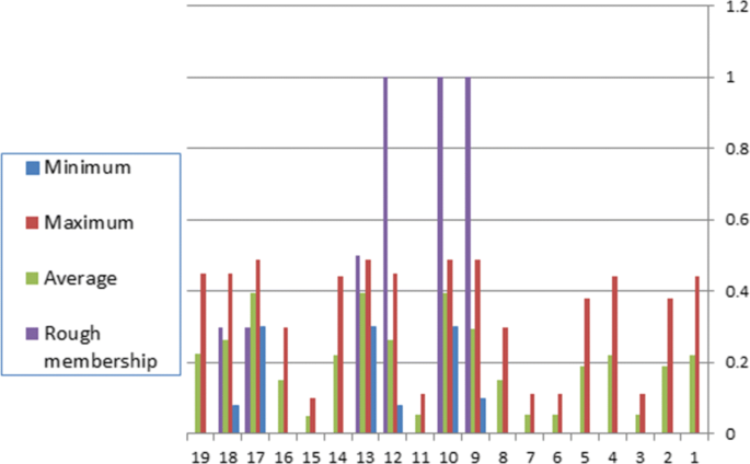
Rough membership for X={x9,x10,x12}
Table 6 Weighed rough membership for X In [14], the decision rules are coded into three qualitative terms, such as low, medium, and high. X is the set of objects that protein has high energy of unfolding.
Case 2: Let Y={x4,x8,x13,x17,x19}. Then, we have:
$$\begin{array}{ccccc} \mu^{C_{1}}_{Y}(x_{1})= 0.30 &\mu^{C_{2}}_{Y}(x_{2})= 0.10 &\mu^{C_{2}}_{Y}(x_{3})= 0.10 &\mu^{C_{1}}_{Y}(x_{4})= 0.30 &\mu^{C_{1}}_{Y}(x_{5})= 0.30\\ \mu^{C_{4}}_{Y}(x_{1})= 0.28 &\mu^{C_{3}}_{Y}(x_{2})= 0.0 &\mu^{C_{3}}_{Y}(x_{3})= 0.0 &\mu^{C_{4}}_{Y}(x_{4})= 0.28 &\mu^{C_{2}}_{Y}(x_{5})= 0.10\\ \mu^{C_{5}}_{Y}(x_{1})= 0.18 &\mu^{C_{5}}_{Y}(x_{2})= 0.18 &\mu^{C_{5}}_{Y}(x_{3})= 0.18 &\mu^{C_{5}}_{Y}(x_{4})= 0.18 &\mu^{C_{3}}_{Y}(x_{5})= 0.0\\ \mu^{C_{7}}_{Y}(x_{1})= 0.18 &\mu^{C_{6}}_{Y}(x_{2})= 0.0 &\mu^{C_{6}}_{Y}(x_{3})= 0.0 &\mu^{C_{7}}_{Y}(x_{4})= 0.18 &\mu^{C_{4}}_{Y}(x_{5})= 0.28\\ \mu^{C_{8}}_{Y}(x_{1})= 0.30 &\mu^{C_{7}}_{Y}(x_{2})= 0.18 &\mu^{C_{7}}_{Y}(x_{3})= 0.18 &\mu^{C_{8}}_{Y}(x_{4})= 0.30 &\mu^{C_{5}}_{Y}(x_{5})= 0.18\\ \mu^{C_{9}}_{Y}(x_{1})= 0.27 &\mu^{C_{8}}_{Y}(x_{2})= 0.30 &\mu^{C_{11}}_{Y}(x_{3})= 0.0 &\mu^{C_{12}}_{Y}(x_{4})= 0.24 &\mu^{C_{6}}_{Y}(x_{5})= 0.0\\ \mu^{C_{14}}_{Y}(x_{1})= 0.28 &\mu^{C_{11}}_{Y}(x_{2})= 0.0 &\mu^{C_{15}}_{Y}(x_{3})= 0.19 &\mu^{C_{14}}_{Y}(x_{4})= 0.28 &\mu^{C_{7}}_{Y}(x_{5})= 0.18 \\ \end{array}$$$$\begin{array}{ccccc} \mu^{C_{15}}_{Y}(x_{1})= 0.19 &\mu^{C_{12}}_{Y}(x_{2})= 0.24 &&\mu^{C_{15}}_{Y}(x_{4})= 0.19 &\mu^{C_{8}}_{Y}(x_{5})= 0.30\\ \mu^{C_{16}}_{Y}(x_{1})= 0.30 &\mu^{C_{16}}_{Y}(x_{2})= 0.30 &&\mu^{C_{16}}_{Y}(x_{4})= 0.30 &\mu^{C_{14}}_{Y}(x_{5})= 0.28\\ \mu^{C_{19}}_{Y}(x_{1})= 0.31 &&&\mu^{C_{18}}_{Y}(x_{4})= 0.27 &\mu^{C_{15}}_{Y}(x_{5})= 0.19\\ &&& \mu^{C_{19}}_{Y}(x_{4})= 0.31 & \mu^{C_{16}}_{Y}(x_{5})= 0.30\end{array}$$and
$$\begin{array}{cccccc} \mu^{C_{2}}_{Y}(x_{6})= 0.10 &\mu^{C_{1}}_{Y}(x_{7})= 0.30 &\mu^{C_{1}}_{Y}(x_{8})= 0.30 &\mu^{C_{1}}_{Y}(x_{9})= 0.30 &\mu^{C_{9}}_{Y}(x_{10})= 0.27\\ \mu^{C_{3}}_{Y}(x_{6})= 0.0 &\mu^{C_{2}}_{Y}(x_{7})= 0.10 &\mu^{C_{2}}_{Y}(x_{8})= 0.10 &\mu^{C_{9}}_{Y}(x_{9})= 0.27 &\mu^{C_{10}}_{Y}(x_{10})= 0.42\\ \mu^{C_{5}}_{Y}(x_{6})= 0.18 &\mu^{C_{3}}_{Y}(x_{7})= 0.0 &\mu^{C_{4}}_{Y}(x_{8})= 0.28 &\mu^{C_{10}}_{Y}(x_{9})= 0.42 &\mu^{C_{12}}_{Y}(x_{10})= 0.24\\ \mu^{C_{6}}_{Y}(x_{6})= 0.0 &\mu^{C_{4}}_{Y}(x_{7})= 0.28 &\mu^{C_{5}}_{Y}(x_{8})= 0.18 &\mu^{C_{12}}_{Y}(x_{9})= 0.24 &\mu^{C_{13}}_{Y}(x_{10})= 0.51\\ \mu^{C_{7}}_{Y}(x_{6})= 0.18 & \mu^{C_{5}}_{Y}(x_{7})= 0.18 &\mu^{C_{7}}_{Y}(x_{8})= 0.18 &\mu^{C_{13}}_{Y}(x_{9})= 0.51 &\mu^{C_{17}}_{Y}(x_{10})= 0.70\\ \mu^{C_{11}}_{Y}(x_{6})= 0.0 &\mu^{C_{6}}_{Y}(x_{7})= 0.0 &\mu^{C_{8}}_{Y}(x_{8})= 0.30 & \mu^{C_{18}}_{Y}(x_{9})= 0.27 &\mu^{C_{18}}_{Y}(x_{10})= 0.27\\ \mu^{C_{15}}_{Y}(x_{6})= 0.19 & \mu^{C_{7}}_{Y}(x_{7})= 0.18 &\mu^{C_{14}}_{Y}(x_{8})= 0.28 & \mu^{C_{19}}_{Y}(x_{9})= 0.31 & \mu^{C_{19}}_{Y}(x_{10})= 0.31\\ &\mu^{C_{8}}_{Y}(x_{7})= 0.30 &\mu^{C_{15}}_{Y}(x_{8})= 0.19 &&\\ &\mu^{C_{14}}_{Y}(x_{7})= 0.28 &\mu^{C_{16}}_{Y}(x_{8})= 0.30 &&\\ &\mu^{C_{15}}_{Y}(x_{7})= 0.19 &\mu^{C_{19}}_{Y}(x_{8})= 0.31 && \\ & \mu^{C_{16}}_{Y}(x_{7})= 0.30 &&&\end{array}$$and
$$\begin{array}{cccccc} \mu^{C_{2}}_{Y}(x_{11})= 0.10 &\mu^{C_{2}}_{Y}(x_{12})= 0.10 &\mu^{C_{9}}_{Y}(x_{13})= 0.27 &\mu^{C_{1}}_{Y}(x_{14})= 0.30 &\mu^{C_{1}}_{Y}(x_{15})= 0.30\\ \mu^{C_{3}}_{Y}(x_{11})= 0.0 &\mu^{C_{4}}_{Y}(x_{12})= 0.28 & \mu^{C_{10}}_{Y}(x_{13})= 0.42 &\mu^{C_{4}}_{Y}(x_{14})= 0.28 &\mu^{C_{3}}_{Y}(x_{15})= 0.0\\ \mu^{C_{6}}_{Y}(x_{11})= 0.0 &\mu^{C_{9}}_{Y}(x_{12})= 0.27 & \mu^{C_{13}}_{Y}(x_{13})= 0.51 &\mu^{C_{5}}_{Y}(x_{14})= 0.18 &\mu^{C_{4}}_{Y}(x_{15})= 0.28\\ \mu^{C_{11}}_{Y}(x_{11})= 0.0 &\mu^{C_{10}}_{Y}(x_{12})= 0.42 & \mu^{C_{17}}_{Y}(x_{13})= 0.70 &\mu^{C_{7}}_{Y}(x_{14})= 0.18 &\mu^{C_{5}}_{Y}(x_{15})= 0.18\\ &\mu^{C_{12}}_{Y}(x_{12})= 0.24 &&\mu^{C_{8}}_{Y}(x_{14})= 0.30 &\mu^{C_{6}}_{Y}(x_{15})= 0.0\\ &\mu^{C_{14}}_{Y}(x_{12})= 0.28 &&\mu^{C_{12}}_{Y}(x_{14})= 0.24 & \mu^{C_{7}}_{Y}(x_{15})= 0.18 \\ &\mu^{C_{18}}_{Y}(x_{12})= 0.27 &&\mu^{C_{14}}_{Y}(x_{14})= 0.28 & \mu^{C_{8}}_{Y}(x_{15})= 0.30\\ &\mu^{C_{19}}_{Y}(x_{12})= 0.31 &&\mu^{C_{15}}_{Y}(x_{14})= 0.19 & \mu^{C_{14}}_{Y}(x_{15})= 0.28\\ &&&\mu^{C_{16}}_{Y}(x_{14})= 0.30 & \mu^{C_{15}}_{Y}(x_{15})= 0.19\\ &&&\mu^{C_{18}}_{Y}(x_{14})= 0.27 & \mu^{C_{16}}_{Y}(x_{15})= 0.30\\ &&&\mu^{C_{19}}_{Y}(x_{14})= 0.31 &\end{array}$$and
$$\begin{array}{cccccc} \mu^{C_{1}}_{Y}(x_{16})= 0.30 &\mu^{C_{10}}_{Y}(x_{17})= 0.42 &\mu^{C_{4}}_{Y}(x_{18})= 0.28 &\mu^{C_{1}}_{Y}(x_{19})= 0.30\\ \mu^{C_{2}}_{Y}(x_{16})= 0.10 &\mu^{C_{13}}_{Y}(x_{17})= 0.51 &\mu^{C_{9}}_{Y}(x_{18})= 0.27 & \mu^{C_{4}}_{Y}(x_{19})= 0.28\\ \mu^{C_{4}}_{Y}(x_{16})= 0.28 &\mu^{C_{17}}_{Y}(x_{17})= 0.70 &\mu^{C_{10}}_{Y}(x_{18})= 0.42 &\mu^{C_{8}}_{Y}(x_{19})= 0.30\\ \mu^{C_{5}}_{Y}(x_{16})= 0.18 &&\mu^{C_{12}}_{Y}(x_{18})= 0.24 & \mu^{C_{9}}_{Y}(x_{19})= 0.27\\ \mu^{C_{7}}_{Y}(x_{16})= 0.18 &&\mu^{C_{14}}_{Y}(x_{18})= 0.28 &\mu^{C_{10}}_{Y}(x_{19})= 0.42\\ \mu^{C_{8}}_{Y}(x_{16})= 0.30 &&\mu^{C_{18}}_{Y}(x_{18})= 0.27 & \mu^{C_{12}}_{Y}(x_{19})= 0.24\\ \mu^{C_{14}}_{Y}(x_{16})= 0.28 &&\mu^{C_{19}}_{Y}(x_{18})= 0.31 & \mu^{C_{14}}_{Y}(x_{19})= 0.28\\ \mu^{C_{15}}_{Y}(x_{16})= 0.19 &&&\mu^{C_{16}}_{Y}(x_{19})= 0.30\\ \mu^{C_{16}}_{Y}(x_{16})= 0.30 &&&\mu^{C_{18}}_{Y}(x_{19})= 0.27\\ \mu^{C_{19}}_{Y}(x_{16})= 0.31 &&&\mu^{C_{19}}_{Y}(x_{19})= 0.31\\ &&&\end{array}$$Now, we evaluate the rough membership for each object which gives a preferable value for the data. This value will be evaluated via minimum, maximum, average, and weighed membership. This can be shown in Table 6 and Fig. 2.
Fig. 2 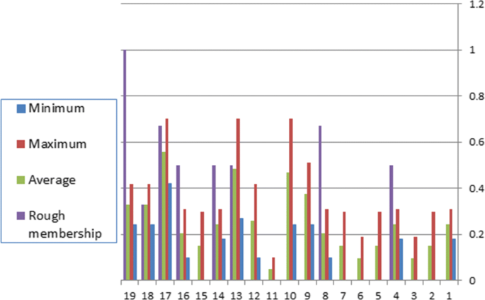
Rough membership for Y={x4,x8,x13,x17,x19}
Y is the set of objects that protein has a medium energy of unfolding. From Table 7, one can show that the objects x9,x10,x12 have a rough membership value 1; this means that a protein has high energy of unfolding. The object x19 in Pawlak reduction had a medium energy of unfolding [14], while from our procedure, x19 has a high energy of unfolding. In the same manner, we can take a set Z of a protein, which has a low energy of unfolding. Through the correlation between objects and decision, there is at least one object in Z which has the medium or the high energy of unfolding. Therefore, the significance of each attribute and degrees of memberships is more precise from Pawlak’s reduction. We can evaluate analogously the quantitative for attributes {a2,a3,a4,a5,a6,a7}.
Table 7 Weighed rough membership for Y


Some properties on a similarity relation
The given algorithm depends on a similarity matrix, general binary relation, and rough membership. So, we study some properties of these notions.
Proposition 1
If R1 and R2 are two different relations, then the degree of similarity is the same.
Proof
A similarity measure between xi and xj is given by \(\text {deg}_{a}(x_{i}, x_{j})= 1- \frac {|a(x_{i})- a(x_{j})|}{|a_{\text {max}}-a_{\text {min}}|}\). Since each of R1 and R2 depends on d, then \(|x_{i} R_{1}|= \sum \limits _{x_{k}\in C_{k}}d_{ij}= |x_{i} R_{2}|\). Therefore, the degree of similarity is the same. □
Proposition 2
If R1⊆R2, then \(\text {deg}_{R_{1}}(x_{i}, x_{j}) \leq \text {deg}_{R_{2}}(x_{i}, x_{j})\), where deg is the degree of similarity relation.
Proof
Since R1⊆R2, then \(|x_{i} R_{1}|= \sum \limits _{x_{k}\in C_{k}}d_{ij}\leq \sum \limits _{x_{k}\in C_{k}} d^{'}_{ij}= |x_{i} R_{2}|\), where dij and \(d^{'}_{ij}\) are the similarity degrees with respect to R1 and R2, respectively. □
Proposition 3
For an IS (U,A), where U is the set of objects and A is the sets of attributes. Then, μXCk(x)=μXCk(y), for every two different objects x,y∈A, every class Ck, and every nonempty set X⊆U.
Proof
Directly from \(\mu ^{C_{k}}_{X}(x)= \frac {\sum \limits _{x\in C_{k}\cap X} d_{ij}}{\sum \limits _{x\in C_{k}}d_{ij}}= \mu ^{C_{k}}_{X}(y)\) □
Remark 1
For an attribute a∈A in an IS (U,A). If μXCk(x)=μXCm(x), k≠m, it is not necessary that Ck=Cm. This is obvious in the problem of our study.
Conclusion and discussion
Chemical data sets have been analyzed using similarity relations. The results are more precise in comparison with the original rough set theory. The description of objects is different from the study in [14]. For example, the decision concerning element x19 in our study has the high energy of unfolding, of which in [14], the energy was the medium of unfolding. This opened the way for applying similarity models in IS which give discrete structure and coincide with the classical case. The model of QSAR of similarity reduction can be applied to a finite set of objects. The approach used here can be applied in any IS with quantitative or qualitative data. Consequently, they are very significant in decision-making [21–24]. The introduced techniques are very useful in application because they open a way for more topological applications from real-life problems.
Availability of data and materials
Not applicable.
Abbreviations
- IS:
-
Information system
- QSAR:
-
Quantitative structure activity relationship
- AAs:
-
Amino acids
References
Pawlak, Z.: Rough sets. Int. J. Inf. Comput. Sci. II, 341–356 (1982). https://doi.org/10.1007/BF01001956.
Pawlak, Z.: Rough sets, Theoretical Aspects of Reasoning About Data. Springer (1991).
Lashin, E. F., Kozae, A. M., Abo Khadra, A. A., Medhat, T.: Rough set theory for topological spaces. Int. J. Approx. Reason. 40, 1–2, 35–43 (2005). https://doi.org/10.1016/j.ijar.2004.11.007.
Salama, A. S., El-Barbary, O. G.: Topological approach to retrieve missing values in incomplete information systems. J. Egypt. Math. Soc. 25, 419–423 (2017). https://doi.org/10.1016/j.joems.2017.07.004.
Pawlak, Z., Skowron, A.: Advances in the Dempster-Shafer theory of evidence. Chapter Rough membership functions, 251-271. Wiley, New York (1994).
Allam, A. A., Bakeir, M. Y., Abo-Tabl, E. A.: New approach for basic rough set concepts, Rough, Sets, Fuzzy Sets, Data Mining, and Granular Computing, Lecture Notes in Artificial Intelligence 3641(Slezak, D., Wang, G., Szczuka, M., Dntsch, I., Yao, Y., eds.)Springer, Berlin (2005).
Salama, A. S.: Some topological properties of rough sets with tools for data mining, IJCSI. Int. J. Comput. Sci. 8(2), 588–595 (2011).
Yao, Y. Y., Zhang, J. P.: Interpreting fuzzy membership functions in the theory of rough sets. In: Rough Sets and Current Trends in Computing, Second International Conference, pp. 82–89. RSCTC 2000 Banff, Canada (2000).
Yu, Z., Wang, D.: Accuracy of approximation operators during covering evolutions. Int. J. Approx. Reason. 117, 1–14 (2020). https://doi.org/10.1016/j.ijar.2019.10.012.
Wang, X. W., Zhang, W. B.: Chemical topology and complexity of protein architectures. Trends Biochem. Sci. 43(10), 806–817 (2018). https://doi.org/10.1016/j.tibs.2018.07.001.
Stepaniuk, J.: Similarity based rough sets and learning. In: Proc. of 5th European Congress on Intelligent Techniques & Soft Computing, pp. 1634–1638 (1997).
Abo-Tabl, E. A.: Rough sets and topological spaces based on similarity. Int. J. Mach. Learn. and Cyber. 4, 451–458 (2013).
Elshenawy, A., El-Sayed, M. K., Elsodany, M.: Weighted membership based on matrix relation. Math. Meth. Appl. Sci., 1–9 (2017). https://doi.org/10.1002/mma.4631.
Walczak, B., Massart, D. L.: Tutorial rough set theory. Chemometr. Intell. Lab. Syst. 47, 1–16 (1999).
Kozae, A. M.: On topology expansions by ideals and applications. Chaos, Solitons and Fractals. 13, 55–60 (2002). https://doi.org/10.1016/S0960-0779(00)00224-1.
Chakraborty, M. K.: Membership function based rough set. Int. J. Approx. Reason. 55, 402–411 (2014). https://doi.org/10.1016/j.ijar.2013.10.009.
Pawlak, Z., Skowron, A.: Rough membership function: a tool for reasoning with uncertainty, Algebraic Methods in Logic and in Computer Science Banach Center Publications, 28, Institute of Mathematics Polish Academy of Sciences Warszawa. 28(1), 135–150 (1993).
El-Sayed, M. K.: Similarity based membership of elements to uncertain concept in information system. Int. Sch. Sci. Res. Innov. 12(3), 58–61 (2018).
Tropsha, A.: Fundamentals of QSAR modeling: basic concepts and applications, Fundamentals of Using QSAR Models and Read-across Techniques in Predictive Toxicology, University of North Carolina. Chapel Hill, USA (2016).
El Tayar, N. E., Tsai, R. -S., Carrupt, P. -A., Testa, B.J. Chem. Soc. Perkin Trans. 2, 79–84 (1992).
Jiang, H., Zhan, J., Chen, D.: Covering based variable precision \(({\mathcal {I}}, {\mathcal {T}})\)-fuzzy rough sets with applications to multi-attribute decision-making. IEEE Trans. Fuzzy Syst. (2018). https://doi.org/10.1109/TFUZZ.2018.2883023.
Zhan, J., Sun, B., Alcantud, J. C. R.: Covering based multigranulation \(({\mathcal {I}}, {\mathcal {T}})\)-fuzzy rough set models and applications in multi attribute group decision-making. Inf. Sci. 476, 290–318 (2019). https://doi.org/10.1016/j.ijar.2013.05.004.
Zhang, L., Zhan, J., Xu, Z.: Covering-based generalized IF rough sets with applications to multi-attribute decision-making. Inf. Sci. 478, 275–302 (2019). https://doi.org/10.1016/j.ins.2018.11.033.
Alharbi, N., Aydi, H., Özel, C., Topal, S.: Rough topologies on classical and based covering rough sets with applications in making decisions on patients with some medical problems Preprint (2020). https://www.researchgate.net/publication/338969347.
Acknowledgements
The author would like to thank the anonymous referees for their helpful comments that improve the presentation of this paper.
Funding
Not applicable.
Author information
Authors and Affiliations
Contributions
All authors jointly worked on the results, and they read and approved the final manuscript.
Ethics declarations
Competing interests
The author declares that there are no competing interests.
Additional information
Publisher’s Note
Springer Nature remains neutral with regard to jurisdictional claims in published maps and institutional affiliations.
Rights and permissions
Open Access This article is licensed under a Creative Commons Attribution 4.0 International License, which permits use, sharing, adaptation, distribution and reproduction in any medium or format, as long as you give appropriate credit to the original author(s) and the source, provide a link to the Creative Commons licence, and indicate if changes were made. The images or other third party material in this article are included in the article’s Creative Commons licence, unless indicated otherwise in a credit line to the material. If material is not included in the article’s Creative Commons licence and your intended use is not permitted by statutory regulation or exceeds the permitted use, you will need to obtain permission directly from the copyright holder. To view a copy of this licence, visit http://creativecommons.org/licenses/by/4.0/.
About this article

Cite this article
El Atik, A.A. Reduction based on similarity and decision-making. J Egypt Math Soc 28, 22 (2020). https://doi.org/10.1186/s42787-020-00078-4
Received:
Accepted:
Published:
DOI: https://doi.org/10.1186/s42787-020-00078-4