Synergy in fertility forecasting: improving forecast accuracy through model averaging

Abstract

Accuracy in fertility forecasting has proved challenging and warrants renewed attention. One way to improve accuracy is to combine the strengths of a set of existing models through model averaging. The model-averaged forecast is derived using empirical model weights that optimise forecast accuracy at each forecast horizon based on historical data. We apply model averaging to fertility forecasting for the first time, using data for 17 countries and six models. Four model-averaging methods are compared: frequentist, Bayesian, model confidence set, and equal weights. We compute individual-model and model-averaged point and interval forecasts at horizons of one to 20 years. We demonstrate gains in average accuracy of 4–23% for point forecasts and 3–24% for interval forecasts, with greater gains from the frequentist and equal weights approaches at longer horizons. Data for England and Wales are used to illustrate model averaging in forecasting age-specific fertility to 2036. The advantages and further potential of model averaging for fertility forecasting are discussed. As the accuracy of model-averaged forecasts depends on the accuracy of the individual models, there is ongoing need to develop better models of fertility for use in forecasting and model averaging. We conclude that model averaging holds considerable promise for the improvement of fertility forecasting in a systematic way using existing models and warrants further investigation.

Introduction

Fertility forecasts are a vital element of population and labour force forecasts, and accurate fertility forecasting is essential for government policy, planning and decision-making regarding the allocation of resources to multiple sectors, including maternal and child health, childcare, education and housing. Though the level of fertility in industrialised countries has at times been of major concern (e.g., Kuczynski (1937); Booth (1986); Longman (2004)), models for forecasting fertility have been developed relatively recently (for an earlier review, see Booth (2006)). Indeed, many of the models used in fertility forecasting were originally designed to smooth age-specific fertility rates or complete the incomplete experience of a single cohort, and relatively few have been used in longer-term forecasting of period fertility rates; further, many are deterministic providing no indication of uncertainty (Bohk-Ewald et al. 2018).

Stochastic models for forecasting period age-specific fertility rates (ASFRs) make use of various time-series extrapolation models and generally involve extensive simulation to take account of covariance in the estimation of uncertainty. The most straightforward approach uses univariate time-series models (see, e.g., Box et al. (2008)) to extrapolate the trend at each age. The main limitation of this approach is inconsistency among age-specific forecasts, possibly producing an implausible age pattern of future fertility. To remedy this, the age pattern is first modelled, and its parameters are then forecast. Parametric models used in forecasting include the beta, gamma, double exponential and Hadwiger functions (see, e.g., Thompson et al. (1989); Congdon (1990); Congdon (1993); Knudsen et al. (1993); Keilman and Pham (2000)), while semi-parametric models include the Coale-Trussell and Relational Gompertz models (see, e.g., Coale and Trussell (1974); Brass (1981); Murphy (1982); Booth (1984); Zeng et al. (2000)). The use of these models is variously limited by parameter un-interpretability, over-parameterization and the need for vector autoregression. Structural change also limits their utility, especially where vector autoregression is involved (Booth 2006).

Nonparametric methods use a dimension-reduction technique, such as principal components analysis, to linearly transform ASFRs to extract a series of time-varying indices to be forecast (see, e.g., Bozik and Bell (1987); Bell (1992); Lee (1993); Hyndman and Ullah (2007); Myrskylä et al. (2013)). This approach parallels the Lee-Carter model and its many variants and extensions in mortality forecasting (see, e.g., Shang et al. (2011)), but has received far less attention. Other contributions include state-space, Bayesian and stochastic diffusion approaches (see, e.g., Rueda and Rodríguez (2010); Myrskylä and Goldstein (2013); Schmertmann et al. (2014)).

The strengths and weaknesses of fertility forecasting models have not been thoroughly evaluated. Noting the absence of guidance on model choice, Bohk-Ewald et al. (2018) compared the point and interval forecast accuracy of 20 major models for fertility forecasting with 162 variants. In the context of completing cohort fertility, their evaluation found that only four methods were consistently more accurate than the constant (no change) model and, among these, complex Bayesian models did not outperform simple extrapolative models. These findings were mostly universal. In earlier research, Shang (2012b) compared several models for fertility forecasting for point and interval forecast accuracies, finding the weighted Hyndman-Ullah model (see the “Six selected models” section) to be marginally more accurate on both counts. While this research is useful in identifying models that perform well based on extensive data, such models may not perform well in every circumstance. Moreover, there is undoubtedly scope for fertility forecasting improvement.

In other areas of forecasting, model averaging (Bates and Granger 1969; Dickinson 1975; Clemen 1989) has been employed to improve point and interval forecast accuracy. However, with the exceptions of Shang (2012a) and Shang and Haberman (2018), model averaging has been neglected in forecasting demographic rates. This paper aims to empirically assess the extent to which forecast accuracy can be improved through model averaging in the context of age-specific fertility forecasting. Our assessment covers 17 countries with varied fertility experience and is based on data series extending back to 1950 or before. We consider six selected models and four methods for selecting model averaging weights.

The structure of this article is as follows. In the “Model averaging” section, we introduce model averaging and briefly present the four methods for selecting weights; the technical details of these methods are given in Appendix A. The data, six selected models and study design are described in the “Data and design” section, and technical details of the six models appear in Appendix B. Based on the accuracy measures discussed in Appendix C, in the “Results” section, we evaluate the point and interval forecast accuracies of the six models and of the four model-averaged forecasts. In the “Model averaging in practice” section, we provide an example of model averaging in forecasting age-specific fertility, using data for England and Wales. Finally, the discussion appears in the “Discussion” section.

Model averaging

The idea of model averaging has been often studied in statistics, dating back to the seminal work by Bates and Granger (1969). A flurry of articles then appeared dedicated to the topic; see Clemen (1989) for a review from a frequentist viewpoint and Hoeting et al. (1999) for a review from a Bayesian perspective. More recent developments in model averaging are collected in the monograph by Claeskens and Hjort (2008). In demographic forecasting, there has been limited usage, but notable exceptions include Smith and Shahidullah (1995), Ahlburg (1998, 2001) and Sanderson (1998) in the context of census tract forecasting.

In essence, the model-averaging approach combines forecasts from a set of two or more models. Because these models may reflect different assumptions, model structures and degrees of model complexity, it is expected that better forecast accuracy can be achieved through averaging. The forecasts from each model are averaged using weights that are specific to each forecast horizon. This is designed to achieve accuracy in the year of the forecast horizon, and not in all years up to and including the horizon year. These model weights are applied at all ages.

In all model-averaging methods, the model-averaged point forecast for horizon h is computed as the weighted mean:

$$\widehat{y}_{n+h|n,\mathrm{M}}=\sum_{\ell=1}^{L}w_{\ell}\widehat{y}_{n+h|n,M_{\ell}}, $$

where M represents the model average, M_ℓ, for $\ell =1,\dots,L$, represents the individual models, $\widehat {y}_{n+h|n,M_{\ell }}$ represents the point forecast at horizon h obtained from model ℓ; $\widehat {y}_{n+h|n,\mathrm {M}}$ represents the model averaged forecast; and $(w_{1}, w_{2}, \dots, w_{L})$ are empirical point forecast weights that sum to 1.

For the model-averaged point forecast $\widehat {y}_{n+h|n,\mathrm {M}}$, its prediction interval is constructed from its variance assuming a normal distribution. Following Burnham and Anderson (2002); Burnham and Anderson (2004), the unconditional variance of the estimator $\tilde {y}_{n+h|n, \mathrm {M}}$ based on the models weighted by empirical interval forecast weights is given by

$$ \widehat{\text{Var}}(\tilde{y}_{n+h|n, \mathrm{M}}) = \left\{\sum^{L}_{i=1}\tilde{w}_{\ell}\left[\widehat{\text{Var}}(\widehat{y}_{n+h|n,M_{\ell}})+(\widehat{y}_{n+h|n,M_{\ell}}-\widehat{y}_{n+h|n, \mathrm{M}})^{2}\right]^{\frac{1}{2}}\right\}^{2}, $$

where $\tilde {w}_{\ell }$ represents the interval forecast weight under model M_ℓ, $\tilde {y}_{n+h|n, \mathrm {M}}$ represents the model-averaged point forecast obtained using interval forecast weights. The first term inside the square brackets measures the variance conditional on model M_ℓ, while the second term measures the squared bias.

The crucial ingredient in model averaging is the empirical weights. The computation of the point forecast weights and interval forecast weights is based on measures of forecast accuracy. The derivation of weights differs by model-averaging method. We employ four methods chosen on the basis of their ability to perform well in mortality forecasting (Shang 2012a; Shang and Haberman 2018). These four methods for computing the weights are briefly described in the following sections. Further details are given in Appendix A.

It should be noted that in this study, the measures of accuracy are further averaged as part of the study design (see the “Study design” section), increasing the reliability and stability of the weights.

A frequentist approach

Under the frequentist approach employed, the accuracy of a point forecast is measured by mean absolute forecast error (MAFE) while the accuracy of an interval forecast is measured by the mean interval score. These measures are described in Appendix C.

In the simple case of a single point forecast for a particular horizon h, MAFE is averaged over age for the year n+h, and the weight is taken to be equal to the inverse of MAFE. Weights are obtained for the set of forecasting models and standardised to sum to 1, giving the standardised weights $(w_{1}, w_{2}, \dots, w_{L})$. Similarly, interval forecast accuracy is based on the mean interval score for year n+h, and the weight is equal to its inverse. For the set of models, weights are standardised to achieve proportionality, giving the standardised weights $(w_{1}, w_{2}, \dots, w_{L})$. Further averaging of MAFE and the mean interval score takes place as a result of study design, before weight calculation.

A Bayesian approach

In Bayesian model averaging, a single set of model weights is used for the point and interval forecasts. The weights are derived from the Bayesian information criterion (BIC) and are thus proportional to model goodness-of-fit and incorporate a penalty for more parameters. Further details appear in Appendix A.

Model confidence set (MCS)

To examine statistical significance among the set of models and select a set of superior models, we consider the MCS procedure. The MCS procedure proposed by Hansen et al. (2011) consists of a sequence of tests of the hypothesis of equal predictive ability (EPA) of two models, eliminating the worse-performing model at each step and resulting in a smaller set of superior models for which the hypothesis is universally accepted. After determining this set of superior models, their forecasts are averaged without weights.

Equal weights

As a baseline approach, we also consider assigning equal weights to all six models. Prior research has shown that including all models in an equal weights (or unweighted) model can yield substantial gains in forecast accuracy. Several studies provide analytical solutions for the conditions under which equal weights provide more accurate out-of-sample forecasts than regression weights (e.g., Einhorn and Hogarth (1975); Davis-Stober (2011)). Equal weights can be advantageous when models fit the data poorly (Graefe 2015).

Data and design

Data sets

The study is based on fertility data for 17 countries. For all but one country, the data were taken from the Human Fertility Database (2020). Australian fertility rates and populations were obtained from Australian Bureau of Statistics (Cat. No. 3105.0.65.001, Table 38); this data set is also available in the rainbow package (Shang and Hyndman 2019) in the statistical software R (R Core Team 2020). The data consist of annual fertility rates by single-year age of women aged 15 to 49 and corresponding population (births to women aged 50 and older are included in births at age 49). The 17 selected countries all have reliable data series commencing in 1950 or earlier, as shown in Table 1, and extending to 2011.

Table 1 Countries and period of data availability

The overall level of fertility has declined in all countries considered. Figure 1 shows that the general decline in total fertility (births per woman calculated as the sum of ASFRs in each year) has not been monotonic. It also indicates that the substantial decline in fertility since 1960 has been stalled or reversed since about 2000. While trends in ASFRs may differ from this overall pattern, total fertility provides the average trend.

Fig. 1

Total fertility of 17 selected countries, where the vertical dotted line divides the in-sample period and the holdout sample period

Six selected models

We select six models used in forecasting fertility. These include three functional time-series models for modelling the schedule of ASFRs, where age is treated as a continuum; and three univariate time-series models to model fertility at each age individually. All models are applied to transformed ASFRs so as ensure non-negative forecast rates.

Functional time-series models

The three models included here stem from the work of Hyndman and Ullah (2007). These models use principal component decomposition with time series forecasting of the time parameter and are similar to the well-known method by Lee and Carter (1992) for modelling and forecasting mortality rates.

The Hyndman-Ullah (HU) model uses smoothed transformed ASFRs. The functional principal component decomposition produces smooth age parameters and corresponding time parameters. Several components are required to adequately describe the data. The time parameters are each modelled using time series methods, providing the forecast.

Two variants of the HU model are also selected. The robust HU model (HUrob) is robust to outliers. The weighted HU model (HUw) gives greater weight to more recent data in order to reduce the potential gap between the last year of observed data and the first year of the forecast. The HU model and its two variants are described in detail in Appendix B.

Univariate time-series models

The three selected univariate time-series models (Box et al. 2008) include two random-walk models and an optimal autoregressive integrated moving average (ARIMA) model and are applied to transformed ASFRs at each age. They are described in detail in Appendix B.

The random-walk models include the random walk (RW) and the random walk with drift (RWD). Each model is applied independently to each age-specific rate. While the RW model assumes a constant underlying rate over time with all deviations assumed to be error, the RWD assumes a constant underlying change in the transformed rates at each age.

The optimal ARIMA model is the model best describing the time series of an age-specific fertility rate based on its own past values, including its own lags and lagged forecast errors. The equation is then used to forecast future values of the series.

Study design

We implement a two-stage design. At the first stage, the six forecasting models are applied to determine model weights based on forecast errors. At the second stage, the six models and their model averages are evaluated. These two stages use different periods of data as illustrated in Fig. 2. We divide the data for each country into an in-sample period ending in 1991 and a holdout sample period, 1992 to 2011.

Fig. 2

Fitting and forecasting periods for weight estimation (stage 1) and model-averaged forecasting (stage 2). The start of the fitting period is determined by data availability or purposive choice

The in-sample data are used in the first stage. We further divide these data into a fitting period and a forecasting period. The initial fitting period ended in 1971, and the forecasting period was 1972 to 1991. Using the data in this fitting period, we fit each model, compute 1-year-ahead to 20-year-ahead forecasts of 35 ASFRs, and calculate forecast errors or information criterion values by comparing the forecasts with observed data in the relevant year. Figure 3 provides an example. Then, we expand the fitting period by one year, and compute 1-year-ahead to 19-year-ahead forecasts, and again calculate forecast errors or information criterion values. This process is repeated until the fitting period extends to 1990. In so doing, we have 20 sets of 1-year-ahead forecast errors, 19 sets of 2-year-ahead forecast errors, $\dots$ and one set of 20-year-ahead forecast errors. These forecast errors are used in the calculation of appropriate weights for the model-averaging approach. In practice, the model-averaging weights are derived from forecast errors averaged over horizon-specific forecasts and over the 17 countries in the study. There is thus one set of six weights for each model-averaging method.

Fig. 3

Comparison of observed data with 1-year-ahead and 20-year-ahead point and interval forecasts of Australian ASFRs based on data for 1921–1971 using the HU model

These forecast errors are used in the calculation of appropriate weights for the model-averaging approach. In the HUw model where geometrically decaying weights are used, the decaying parameter, λ, is estimated from data for 1960 to 1981, for $h=1,\dots,20$. The overlap with the in-sample forecasting period (1970 to 1991) is inevitable given short data series for some countries.

At the second stage, the entire dataset is used. The initial fitting period ended in 1991, and the forecasting period was 1992 to 2011. An expanding fitting period is again employed, producing forecasts for horizons of 1 to 20 years. Point and interval forecasts are produced for the six forecasting models and for the model-averaged forecasts using each of the four model averaging methods. Forecast errors are again calculated by comparison with observed data and used in the evaluation of point and interval forecast accuracy as measured by MAFE and the mean interval score, respectively.

Implementation of the HU models presented in this paper is straightforward with the readily available R package demography (Hyndman 2019). Point and interval forecasts based on the RW, RWD and ARIMA models can be obtained via the rwf and auto.arima functions in the forecast package (Hyndman 2020). The computational code in R for the entire analysis is available upon request.

Results

Point forecast accuracy

In Table 2, we present the out-of-sample point forecast accuracy based on 1-year-ahead to 20-year-ahead MAFEs, which are averaged over ages, years in the forecasting period and countries. Irregularities at longer horizons are due to two factors: the small number of forecasts involved (see Fig. 3) and the fact that they are based entirely on fitting periods ending in 1986 to 1990, a period of changing trends in several countries (see Fig. 1).

Table 2 MAFEs (×100) for ASFRs for 1-year-ahead to 20-year-ahead point forecasts by model/method and forecast horizon

As shown in Table 2, we find that gains in forecast accuracy due to model averaging have been achieved at longer (h>7) rather than shorter forecast horizons. The median value of MAFE is 0.0096 for the model-averaged forecasts with weights selected by the frequentist approach and equal weights, which indicates gains in accuracy over the six models of 4 to 23%. By contrast, the model averaging methods based on the Bayesian approach and MCS do not perform well.

Interval forecast accuracy

In Table 3, we present the mean interval scores for the 1-year-ahead to 20-year-ahead forecasts. As expected, the mean interval score increases with the forecast horizon, reflecting the loss of interval forecast accuracy as the horizon increases. For short horizons, the model-averaged interval forecasts perform less well than individual models, and the Bayesian and MCS approaches are briefly superior. For horizons of 7 or more years, however, the frequentist and equal weights approaches consistently out-perform the individual models and the more complex model-averaging approaches. Across all horizons, the smallest median (5.11) of the mean interval scores (×100) occurs for the model-averaged forecasts based on the frequentist and equal weights approaches.

Table 3 Mean interval score (×100) for ASFRs for 1-year-ahead to 20-year-ahead interval forecasts by model/method and forecast horizon

Model averaging in practice

To illustrate the application of model averaging to potentially achieve greater forecast accuracy, we use data for England and Wales for 1938 to 2016 and produce frequentist model-averaged point and interval forecasts for horizons of one year and 20 years, based on the six models. At the first stage, horizon-specific weight estimation is based on fitting periods commencing in 1938 and ending successively in 1996 to 2015, with the corresponding forecasting periods starting in 1997 to 2016. In Table 4, we present empirical weights for producing point and interval frequentist model-averaged forecasts. These weights vary little across models, indicating that the six models do not differ appreciably in accuracy. Further, for each model, the point forecast weights and interval forecast weights are roughly equal, showing that the point and interval forecasts are compatible with each other. The fact that the weights differ little across horizons indicates that, in this example, the models do not gain or lose relative advantage over the forecasting period.

Table 4 Point-forecast and interval-forecast frequentist model-averaging weights for fertility rates in England and Wales by model and horizon

At the second stage, the fitting period is 1938 to 2016, and the forecasts are produced using the empirical weights obtained at the first stage. The 1-year-ahead and 20-year-ahead model-averaged point and interval forecasts of age-specific fertility are shown in Fig. 4. The 20-year-ahead point forecast portrays a shift in fertility rates to older ages, continuing the previous trend. However, the shift is more pronounced before than after the mode, which changes little, indicating that the tempo effect is nearing the end of its course. Additionally, this forecast substantially reduces the bulge in fertility rates at young ages seen in recent decades (Chandola et al. 1999).

Fig. 4

Point and 80% interval forecasts of age-specific fertility rates in England and Wales, based on data for 1938 to 2016 using model averaging with frequentist weights (in the first row) and BIC weights (in the second row)

Discussion

This paper has used computational methods to demonstrate that the accuracy of point and interval forecasts for age-specific fertility can be improved through model averaging. The investigation involved four methods for the empirical determination of the weights to be used in model averaging for both the point forecast and interval forecast. Six models produced the initial set of age-specific fertility forecasts. Among the four model averaging approaches compared, the frequentist and equal weights approaches performed best on average, over 17 countries and forecast horizons of 1 to 20 years. This evaluation used weights derived from the accuracy of forecasts for 1992 to 2011 based on a long series of observations up to 1991. The frequentist and equal weights approaches produced gains in point forecast accuracy of 4 to 23% over the six individual models. However, the Bayesian and MCS approaches produced reductions of up to 10%, though some gains were achieved. For the interval forecast, the frequentist and equal weights approaches also produced the greatest improvement in accuracy, with gains of 3 to 24%. Again, the Bayesian and MCS approaches produced the least gains and some losses in forecast accuracy.

These results hold considerable promise for the improvement of fertility forecasting in a systematic way using existing models. The frequentist approach and the equal weights approach both offer a simple way to implement model averaging. Combined with the findings of Bohk-Ewald et al. (2018) that simple forecasting models are as accurate as the most complex, it would seem that improved accuracy can be readily achieved through simple model averaging of simple models. The often cited impediment to the implementation of model averaging, namely complexity, is thus largely removed. To further assist the uptake of model averaging, we look forward to software facilitating its application in fertility forecasting.

Model-averaging approaches

Among the four approaches for the selection of weights, the frequentist and equal weights approaches performed much better than the more complex Bayesian and MCS approaches. The superior performance of the frequentist approach can be attributed to the fact that it assigns weights based on in-sample forecast accuracy. Since ASFRs change in limited ways across age and time, it can be expected that a model that produces smaller in-sample point and interval forecast errors will also produce smaller out-of-sample errors. The performance of the equal weights approach is consistent with previous research (Graefe 2015). It is noted that variation in accuracy across models in Tables 2 and 3 is somewhat limited, partially explaining the superior performance of the equal weights approach. The poor performance of the Bayesian approach can be attributed to the fact that the weights are determined based on in-sample goodness of fit rather than in-sample forecast errors, given that model goodness of fit is not a good indicator of forecast accuracy (Makridakis et al. 2020). The poor performance of the MCS approach can be attributed to the 85% confidence level employed. With a higher confidence level, the MCS method would have selected more accurate models.

Advantages of model averaging

An essential advantage of model averaging is its synergy. In other words, improvements in forecast accuracy can be achieved while using existing methods. Further, in order to achieve optimal accuracy, the ’mix’ of the set of models employed is allowed to change over the forecasting period by using horizon-specific weights favouring more accurate methods. Thus, a model that is highly accurate in the short-term but inaccurate in the long term (or vice versa) can be included in the set of models without jeopardising the accuracy of the model-averaged forecast. This allows the forecaster to make use of a wide range of models and approaches including those that might otherwise be regarded as unsuitable because of their horizon-limited accuracy. Moreover, the weights determining the mix of models is empirical, removing an element of subjectivity in model choice, though a model must of course be included in the initial set of models if it is to be considered at all.

In theory, forecast accuracy is improved by taking relevant additional information into account, most often in the form of other data, such as in the case of joint forecasting of the fertility of a group of countries (Ortega and Poncela 2005). In model averaging, given a single set of data, the additional information encompasses the features of multiple forecasting models. Model averaging can be expected to improve forecast accuracy because the strengths of different assumptions, model structures and degrees of model complexity are essentially combined through weighting that assigns greater weight to more accurate models. In other words, the model-averaged forecasts are more robust to model misspecification.

This advantage might also be expected to increase with the forecast horizon. For any model, uncertainty increases with forecast horizon because the relevant experience in the increasingly distant fitting period becomes more and more attenuated. The effects of model misspecification may be cumulated over time or increasingly accentuated. By using model averaging, the different effects of model misspecification are averaged rather than cumulated, potentially resulting in reduced uncertainty, especially when counterbalancing occurs, and curtailing the extent to which uncertainty increases with forecast horizon. Our results provide some evidence of a greater model-averaging advantage at longer horizons. The model-averaged point and interval forecasts gain ground as forecast horizon increases in terms of accuracy in relation to their six constituent forecasts (see Tables 2 and 3).

Model averaging can also be expected to improve the reliability of forecast accuracy because as an average its range is limited. The model averaging approaches may not be the most accurate forecast among the set, but they are not likely to be the least accurate. In effect, model averaging imposes a lower bound on point and interval forecast accuracy. When the weights are derived empirically based on forecast accuracy from past data, model average accuracy can be expected to be relatively high and can be more accurate than any individual model. An example is seen in Table 3.

It is important to note that these advantages of model averaging hold for any set of models designed to predict period or cohort fertility behaviour at any level of detail. In other words, it is not a requirement that the forecasting models are purely extrapolative, as in this paper. Models based on other approaches such as expert judgement (e.g., Lutz et al. (1996)) and explanation (e.g., Ermisch (1992)) as well as Bayesian modelling (e.g., Schmertmann et al. (2014)) can also be used in model averaging in order to take into account their different strengths in predicting fertility behaviour. Indeed, the traditional ‘medium’ fertility assumption could be included in the set of models.

Limitations

A limitation of this study is that only six models from two families were considered. The set of models included in model averaging will influence the outcome. In this study, we included the RWD, although its appropriateness for longer-term fertility forecasting is limited because of changing trends (Myrskylä et al. 2013) and potential inconsistencies arising from independent forecasting of age-specific rates (Bell 1988). The study confirms the RWD to be least accurate among the six models for both point and interval forecasts. Similarly, the RW is less appropriate for longer horizons because of changing trends. Despite these limitations of the selected models, gains in forecast accuracy were achieved through model averaging. With a larger set of models, greater gains may be achieved because a more diverse range of assumptions and model structures would be taken into account.

A further limitation, arising from data availability, is the focus on period fertility rates, although it is period rates that are used in population projection. Cohort fertility rates have the advantage of describing the fertility behaviour of women over their life course, while parity-specific period rates would provide useful detail to improve model accuracy. Unfortunately, lengthy annual time series of cohort data and parity-specific period data are not available for most of the selected countries, precluding their use in forecasting.

Future research

The findings of this research suggest that model averaging is a potentially fruitful approach to improving the accuracy of fertility forecasting, using models that already exist. A useful technical extension in the case of the frequentist approach to model averaging would be to develop a single set of weights based on a collective criterion incorporating both point and interval forecast accuracy. Additionally, a potential direction for further technical development is to examine other ways of combining models (bagging, boosting and stacking, for example) to achieve greater accuracy than any of the individual models (Bates and Granger 1969).

Based on our findings, we conclude that in the context of fertility forecasting the model-averaging approach warrants further examination using a more extensive range of models and considering both period and cohort data. The choice of potential models is extensive (Booth 2006; Bohk-Ewald et al. 2018) and could usefully include short-term models and those based on explanation and expert opinion. Examination of the weights assigned to different models over time may help to increase understanding of fertility change. Further insights may be gained from the application of model averaging to forecasting total fertility (Saboia 1977; Ortega and Poncela 2005; Alkema et al. 2011), with comparisons of accuracy between direct and indirect forecasting of this aggregate measure.

Finally, we note that optimal forecast accuracy is unlikely to be achieved by preselecting an approach or particular models, but rather is to be found in applying model averaging to a wide range of models encompassing differing strengths in predicting human behaviour. However, while model averaging can be expected to improve forecast accuracy beyond that of the individual models, it is also the case that the accuracy of the individual models broadly determines the range of accuracy that the model-averaged forecast might achieve. Thus, while the prospect of increased accuracy in fertility forecasting is enhanced by the potential of model averaging, the addition of model averaging to the forecasting toolset does not absolve demographers from striving to better understand and model fertility behaviour.

Appendix A: Model averaging methods: technical details

Model averaging involves the computation of weighted means for the point forecast and the interval forecast. Depending on the model-averaging method employed, the weights may be the same for point and interval forecasting, or they may differ. The derivation of weights is described below for the two more complex methods employed in this study, the Bayesian and model confidence set approaches. Full details of the frequentist approach and the use of equal weights appear in the “A frequentist approach” and “Equal weights” sections.

A Bayesian viewpoint

Among the models in the set, let one be considered the correct model, and let $\theta _{1},\theta _{2},\dots,\theta _{L}$ be the vector of parameters associated with each model. Let Δ be the quantity of interest, such as the combined forecast of ASFRs; its posterior distribution given the observed data, D, is

$$\begin{array}{*{20}l} \text{Pr}(\Delta|D) &= \sum^{L}_{i=1}\text{Pr}(\Delta|M_{\ell},D)\text{Pr}(M_{\ell}|D) \\ &=\sum^{L}_{i=1}\text{Pr}(\Delta|M_{\ell},D) \frac{\text{Pr}(D|M_{\ell})\text{Pr}(M_{\ell})}{\sum^{L}_{l=1}\text{Pr}(D|M_{l})\text{Pr}(M_{l})}, \end{array} $$

where $\text {Pr}(D|M_{\ell })=\int \text {Pr}(D|\theta _{\ell },M_{\ell })\text {Pr}(\theta _{\ell }|M_{\ell })d\theta _{\ell }$ and θ_ℓ represents the parameters in M_ℓ, Pr(θ_ℓ|M_ℓ) is the prior density of θ_ℓ under model M_ℓ, Pr(D|θ_ℓ,M_ℓ) is the likelihood, and Pr(M_ℓ) is the prior probability that M_ℓ is the true model.

Given diffuse (also known as non-informative) priors and equal model prior probabilities, the weights for Bayesian model averaging are approximately

$$\begin{array}{*{20}l} w_{\ell} = \tilde{w}_{\ell} = \frac{\exp(-\frac{1}{2}\text{BIC}_{\ell})}{\sum^{L}_{\ell=1}\exp(-\frac{1}{2}\text{BIC}_{\ell})}, \qquad \ell=1,\dots,L, \end{array} $$

(1)

where $\text {BIC}_{\ell } = 2\mathcal {L}_{\ell }+\log (n)\eta _{\ell }$, $\mathcal {L}_{\ell }$ is the negative of the log-likelihood, η_ℓ is the number of parameters in model ℓ, n represents the number of years in the fitting period, and BIC _ℓ is the Bayesian information criterion for model ℓ which can be used as a simple and accurate approximation of the log Bayes factor (see also Kass and Wasserman (1995); Kass and Raftery (1995); Raftery (1995); Burnham and Anderson (2002); Burnham and Anderson (2004); Ntzoufras (2009), Section 11.11). In the case of least squares estimation with normally distributed errors, BIC can be expressed as

$$\text{BIC}_{\ell} = n\log(\widehat{\sigma}^{2}) + \log(n)\eta_{\ell}, $$

where $\widehat {\sigma }^{2} = \sum ^{n}_{i=1}(\widehat {\varepsilon }_{i})^{2}/n$ and $(\widehat {\varepsilon }_{1},\dots,\widehat {\varepsilon }_{n})$ are the residuals from the fitted model. The BIC_ℓ values are not interpretable, as they contain arbitrary constants and are much affected by sample size. We thus adjust BIC_ℓ by subtracting the minimum $\{\text {BIC}_{\ell }; \ell =1,\dots,L\}$. The adjusted BIC_ℓ is used in (1).

Model confidence set (MCS)

As the equal predictive ability (EPA) test statistic can be evaluated for any loss function, we adopt the tractable absolute error measure. The procedure begins with an initial set of models of dimension L encompassing all the models considered, $M_{0} = \{M_{1}, M_{2}, \dots, M_{L}\}$. For a given confidence level, a smaller set, the superior set of models $\widehat {M}_{1-\alpha }^{*}$ is determined where m^∗≤m. The best scenario is when the final set consists of a single model, i.e., m=1. Let l_ℓ,t denote forecast error for model ℓ at time t, and let d_ℓτ,t denote the loss differential between two models ℓ and j, that is

$$d_{\ell \tau,t} = l_{\ell,t} - l_{\tau,t}, \qquad \ell, \tau=1,\dots,L, \quad t=1,\dots,n, $$

and calculate

$$d_{\ell\cdot,t} = \frac{1}{L-1}\sum_{\tau\in \mathrm{M}}d_{\ell\tau,t}, $$

as the loss of model ℓ relative to any other model τ at time point t. The EPA hypothesis for a given set of M models can be formulated in two ways:

$$\begin{array}{*{20}l} \mathrm{H}_{\text{0,M}}: c_{\ell\tau}&=0, \qquad \text{for all}\quad \ell, \tau = 1,2,\dots,L\notag\\ \mathrm{H}_{\text{A,M}}: c_{\ell\tau}&\neq 0, \qquad \text{for some}\quad \ell, \tau = 1,2,\dots,L. \end{array} $$

(2)

or

$$\begin{array}{*{20}l} \mathrm{H}_{\text{0,M}}: c_{\ell.}&=0, \qquad \text{for all}\quad \ell, \tau = 1,2,\dots,L\notag\\ \mathrm{H}_{\text{A,M}}: c_{\ell.}&\neq 0, \qquad \text{for some}\quad \ell, \tau = 1,2,\dots,L. \end{array} $$

(3)

where c_ℓτ=E(d_ℓτ) and c_ℓ.=E(d_ℓ.) are assumed to be finite and time independent. Based on c_ℓτ or c_ℓ., we construct two hypothesis tests as follows:

$$ t_{\ell\tau} = \frac{\overline{d}_{\ell\tau}}{\sqrt{\widehat{\text{Var}}\left(\overline{d}_{\ell\tau}\right)}}, \qquad t_{\ell.} = \frac{\overline{d}_{\ell.}}{\sqrt{\widehat{\text{Var}}\left(\overline{d}_{\ell.}\right)}}, $$

(4)

where $\overline {d}_{\ell.} = \frac {1}{L-1}\sum _{\tau \in \mathrm {M}}\overline {d}_{\ell \tau }$ is the sample loss of ℓth model compared to the averaged loss across models in the set M, and $\overline {d}_{\ell \tau } =\frac {1}{n}\sum ^{n}_{t=1}d_{\ell \tau,t}$ measures the relative sample loss between the ℓth and τth models. Note that $\widehat {\text {Var}}\left (\overline {d}_{\ell.}\right)$ and $\widehat {\text {Var}}\left (\overline {d}_{\ell \tau }\right)$ are the bootstrapped estimates of $\text {Var}\left (\overline {d}_{\ell.}\right)$ and $\text {Var}\left (\overline {d}_{\ell \tau }\right)$, respectively. From Hansen et al. (2011) and Bernardi and Catania (2018), we perform a block bootstrap procedure with 5000 bootstrap samples, where the block length is given by the maximum number of significant parameters obtained by fitting an AR(p) process on all the d_ℓτ term. For both hypotheses in (2) and (3), there exist two test statistics:

$$ T_{\text{R,M}} = \max_{\ell,\tau\in \mathrm{M}}|t_{\ell\tau}|,\qquad T_{\max, \mathrm{M}} = \max_{\ell\in \mathrm{M}} t_{\ell}, $$

(5)

where t_ℓτ and t_ℓ. are defined in (4).

The selection of the worse-performing model is determined by an elimination rule that is consistent with the test statistic,

$$e_{\text{R,M}} = \underset{\ell\in M}{\text{argmax}}\left\{\sup_{\tau\in M}\frac{\overline{d}_{\ell\tau}}{\sqrt{\widehat{\text{Var}}\left(\overline{d}_{\ell\tau}\right)}}\right\},\qquad e_{\max, \mathrm{M}} = \underset{\ell\in M}{\text{argmax}} \frac{\overline{d}_{\ell.}}{\widehat{\text{Var}}\left(\overline{d}_{\ell.}\right)}. $$

To summarise, the MCS procedure to obtain a superior set of models consists of the following steps:

• 1) Set M=M₀;

• 2) If the null hypothesis is accepted, then the final model M^∗=M; otherwise, use the elimination rules defined in (5) to determine the worst model;

• 3) Remove the worst model and go to step 2).

In a particular case of the MCS approach, a lower confidence level results in the inclusion of all models without weights. With a higher confidence level, the MCS approach selects only the most accurate model.

Appendix B: Selected models: technical details

We introduce the six models and describe the calculation of point and interval forecasts for ASFRs. In order to ensure non-negative predictions, prior to modelling, the ASFRs are first transformed using the Box-Cox transformation which is defined as

$$m_{t}(x_{i}) = \left\{ \begin{array}{ll} \frac{1}{\kappa}\left([f_{t}(x_{i})]^{{\kappa}-1}\right) & \text{if}\ 0<\kappa \leq 1;\\ \ln[f_{t}(x_{i})] & \text{if}\ \kappa = 0 \end{array}\right. \quad i=1,2,\dots,p,\quad t=1,2\dots,n, $$

where f_t(x_i) represents the observed ASFR at age x_i in year t, m_t(x_i) represents the transformed ASFR, and κ is the transformation parameter. Following Hyndman and Booth (2008) and Shang (2015), we use κ=0.4 as it gave relatively small holdout sample forecast errors on the untransformed scale.

Hyndman-Ullah (HU) model and two variants

The HU model (Hyndman and Ullah 2007) is described below, along with the defining features of its two variants, the robust HU model (HUrob) and the weighted HU model (HUw).

• The transformed ASFRs are first smoothed using a concave regression spline (for details, see Hyndman and Ullah (2007); Shang et al. (2016)). We assume an underlying continuous and smooth function {s_t(x);x∈[x₁,x_p]} that is observed with error at discrete ages,

  $$m_{t}(x_{i}) = s_{t}(x_{i}) + \sigma_{t}(x_{i})\varepsilon_{t,i}, \qquad \text{for}\quad i=1,2,\dots,p,\quad t=1,2\dots,n, $$

  where σ_t(x_i) allows the amount of noise to vary with x_i in year t, and ε_t,i is an independent and identically distributed (iid) standard normal random variable. As an example, Fig. 5 displays the original and smoothed Australian ASFRs.

  Fig. 5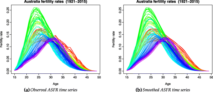

  

  Observed and smoothed ASFRs for Australia, 1921 to 2015. The data are represented chronologically by the colours of the rainbow from red to violet (most recent)

• Given the set of continuous and smooth curves $\{s_{1}(x),s_{2}(x),\dots,s_{n}(x)\}$, the mean function a(x) is estimated by

  $$\widehat{a}(x)=\sum^{n}_{t=1}\varpi_{t}s_{t}(x), $$

  where ϖ_t=1/n represents equal weighting in the HU and HUrob models. In the HUw model, $\{\varpi _{t}=\lambda (1-\lambda)^{n-t},t=1,2,\dots,n\}$ represents a set of geometrically decaying weights (on the selection of optimal λ, see Hyndman and Shang (2009)). The distinguishing feature of the HUw model is that forecasts are based more heavily on recent data.

• Using functional principal components analysis, the set of continuous and smooth curves $\left \{s_{t}(x);t=1,2,\dots,n\right \}$ is decomposed into orthogonal functional principal components and their uncorrelated scores:

  $$s_{t}(x) = \widehat{a}(x) + \sum^{J}_{j=1}\widehat{b}_{j}(x)\widehat{k}_{t,j}+\widehat{e}_{t}(x), $$

  where $\left \{\widehat {b}_{1}(x),\widehat {b}_{2}(x),\dots,\widehat {b}_{J}(x)\right \}$ represents a set of weighted (as above) functional principal components; $\left \{\widehat {k}_{t,1},\widehat {k}_{t,2},\dots,\widehat {k}_{t,J}\right \}$ is a set of uncorrelated scores; $\widehat {e}_{t}(x)$ is the estimated error function with mean zero; and J<n is the number of retained functional principal components. Following Hyndman and Booth (2008), we use J=6 as this has been shown to be sufficiently large to produce iid residuals with a mean of zero and finite variance.

  The HUrob model uses $\widehat {e}_{t}(x)$ to provide information about possible outlying curves. If a curve has a more considerable value of integrated square error, it indicates that this curve may be considered as an outlier that generates from a different data generating process than the rest of the observations. An example of this is fertility rates during the baby boom when sharp temporal increases occurred. Computationally, we use the hybrid algorithm of Hyndman and Ullah (2007) with 95% efficiency (where the most outlying 5% of the data are removed).

• By conditioning on the observed data ${\mathcal {I}}=\left \{m_{1}(x_{i}),\dots,m_{n}(x_{i})\right \}$ and the set of estimated functional principal components ${B}=\left \{\widehat {b}_{1}(x),\dots,\widehat {b}_{J}(x)\right \}$, the h-year-ahead point forecast of m_n+h(x) can be expressed as

  $$\widehat{m}_{n+h|n}(x)=\mathrm{E}[m_{n+h}(x)|{\mathcal{I}},{B}]=\widehat{a}(x)+\sum^{J}_{j=1}\widehat{b}_{j}(x)\widehat{k}_{n+h|n,j}, $$

  where $\widehat {k}_{n+h|n,j}$ denotes the h-year-ahead forecast of k_n+h,j using a univariate time-series model, such as an optimal autoregressive integrated moving average (ARIMA) model (see the “Optimal ARIMA model” section). Note that multivariate time-series forecasting models, such as vector autoregressive and vector autoregressive moving average models, can also be used to forecast principal component score (see, e.g., Aue et al. (2015)).

  Because of the orthogonality of the functional principal components, the overall forecast variance can be approximated by the sum of four variances:

  $$ \text{Var}[m_{n+h}(x)|{\mathcal{I}},{B}]\approx \widehat{\sigma}_{a}^{2}(x)+\sum^{J}_{j=1}[\widehat{b}_{j}(x)]^{2}u_{n+h|n,j}+v(x)+\sigma_{n+h}^{2}(x), $$

  (6)

  where $\widehat {\sigma }_{a}^{2}(x)$ is the variance of the mean function, estimated from the difference between the sample mean function and the smoothed mean function; $\left [\widehat {b}_{j}(x)\right ]^{2}u_{n+h|n,j}$ is the variance of jth estimated functional principal component decomposition where $u_{n+h|n,j}=\text {Var}\left (k_{n+h,j}|\widehat {k}_{1,j},\dots,\widehat {k}_{n,j}\right)$ can be obtained from the univariate time-series models used for forecasting scores; v(x) is the model error variance estimated by averaging $\{\widehat {e}^{2}_{1}(x),\dots,\widehat {e}_{n}^{2}(x)\}$ for each x, and $\sigma _{n+h}^{2}(x)$ is the smoothing error variance estimated by averaging $\{\widehat {\sigma }_{1}^{2}(x),\dots,\widehat {\sigma }_{n}^{2}(x)\}$ for each x. The prediction interval is constructed via (6) on the basis of normality.

Univariate time-series models

The three selected univariate time-series models (Box et al. 2008) are applied to transformed ASFRs at each age.

Random-walk models For each age x_i, the random walk (RW) and random walk with drift (RWD) models are

$$m_{t+1}(x_{i})=c+m_{t}(x_{i})+e_{t+1}(x_{i}), $$

where c represents the drift term capturing a possible trend in the data (in the RW model c=0), and e_t+1(x_i) represents the iid normal error with a mean of zero.

The h-year-ahead point forecast and total variance used for constructing the prediction interval are given by

$$\begin{array}{*{20}l} \widehat{m}_{n+h|n}(x_{i})&=\mathrm{E}[m_{n+h}(x_{i})|m_{1}(x_{i}),\dots,m_{n}(x_{i})]=ch+m_{n}(x_{i}),\\ \text{Var}[\widehat{m}_{n+h|n}(x_{i})]&= \text{Var}[m_{n+h}(x_{i})|m_{1}(x_{i}),\dots,m_{n}(x_{i})]=\text{Var}[m_{n}(x_{i})]+\text{Var}[e_{n+h}(x_{i})], \end{array} $$

where h represents the forecast horizon.

Optimal ARIMA model An ARIMA (p,d,q) model has autoregressive components of order p and moving average components of order q, with d being the degree of difference needed to achieve stationarity (Box et al. 2008). The model can be expressed as

$${}\Delta^{d}m_{t}(x_{i}) = c+\sum^{p}_{\upsilon=1}\beta_{\upsilon}\Delta^{d}m_{t-\upsilon}(x_{i})+\omega_{t}(x_{i})+\sum^{q}_{j=1}\psi_{j}\omega_{t-j}(x_{i}),\qquad t=\max(p,q)+1,\dots,n, $$

where Δ^dm_t(x_i) represents the stationary time series after applying the difference operator of order d, c is the drift term; $\{\beta _{1},\dots,\beta _{p}\}$ represents the coefficients of the autoregressive components; $\{\psi _{1},\dots,\psi _{q}\}$ represents the coefficients of the moving average components; and ω_t(x_i) is a sequence of iid random variables with mean zero and variance $\sigma _{\omega }^{2}$.

We use the auto.arima algorithm (Hyndman and Khandakar 2008) in the forecast package (Hyndman et al. 2020) to select the optimal orders based on the corrected Akaike information criterion, and then estimate the parameters by maximum likelihood. The 1-year-ahead point and interval forecasts are given by

$$\begin{array}{*{20}l} \Delta^{d}\widehat{m}_{n+1|n}(x_{i}) = \mathrm{E}[m_{n+1}(x_{i})|m_{1}(x_{i}),\dots,m_{n}(x_{i})]&=c+\sum^{p}_{\upsilon=1}\widehat{\beta}_{\upsilon} \Delta^{d}m_{n+1-\upsilon}(x_{i}), \end{array} $$

(7)

$$\begin{array}{*{20}l} \text{Var}[m_{n+1}(x_{i})|m_{1}(x_{i}),\dots,m_{n}(x_{i})]&=\widehat{\sigma}_{\omega}^{2}\left(1+\widehat{\psi}_{1}^{2}+\dots+\widehat{\psi}_{q}^{2}\right). \end{array} $$

(8)

For the h-year-ahead forecasts, (7) and (8) are applied iteratively.

Appendix C: Forecast accuracy evaluation

Evaluation of point forecast accuracy

Following Booth et al. (2006) and Shang et al. (2011), we use MAFE to measure point forecast accuracy. MAFE is the average of absolute error, |actual−forecast|, across countries (in this study, $g=1,\dots,17$), years in the forecasting period and ages; it measures forecast precision regardless of sign.

$$\text{MAFE}_{h} = \frac{1}{17\times (21-h)\times 35}\sum^{17}_{g=1}\sum^{n+20-h}_{r=n}\sum^{35}_{i=1}\left|m_{r+h}(x_{i})-\widehat{m}_{r+h|r}(x_{i})\right|, $$

where h denotes forecast horizon, m_r+h|r(x_i) represents the actual ASFR at age x_i in the forecasting period, and $\widehat {m}_{r+h}(x_{i})$ represents the forecast. Note that x₁ corresponds to age 15, and x₃₅ corresponds to age 49.

Evaluation of interval forecast accuracy

To assess interval forecast accuracy, we use the interval score of Gneiting and Raftery (2007) (see also Gneiting and Katzfuss (2014)). For each year in the forecasting period, 1-year-ahead to 20-year-ahead prediction intervals were calculated at the 80% nominal coverage probability, with lower and upper bounds that are predictive quantiles at 10% and 90%. As defined by Gneiting and Raftery (2007), a scoring rule for the interval forecast at age x_i is expressed as

$$\begin{array}{*{20}l} {}S_{\alpha}& \left[\widehat{m}_{r+h|r}(x_{l}),\widehat{m}_{r+h|r}(x_{u});m_{r+h}(x_{i})\right] = \left[\widehat{m}_{r+h|r}(x_{u})-\widehat{m}_{r+h|r}(x_{l})\right]\\&\quad+\frac{2}{\alpha}\left[\widehat{m}_{r+h|r}(x_{l})-m_{r+h}(x_{i})\right]\\ & \mathbbm{1}\left\{m_{r+h}(x_{i})<\widehat{m}_{r+h|r}(x_{l})\right\}\,+\, \frac{2}{\alpha}\left[m_{r+h}(x_{i})-\widehat{m}_{r+h|r}(x_{u})\right]\mathbbm{1}\left\{m_{r+h}(x_{i})>\widehat{m}_{r+h|r}(x_{u})\right\}, \end{array} $$

where α (customarily 0.2) denotes the level of significance, $\widehat {m}_{r+h|r}(x_{l})$ and $\widehat {m}_{r+h|r}(x_{u})$ represent the lower and upper prediction intervals at age x_i in the relevant forecasting period and country. The interval score rewards a narrow prediction interval, if and only if the true observation lies within the prediction interval. The optimal score is achieved when m_r+h(x_i) lies between $\widehat {m}_{r+h|r}(x_{l})$ and $\widehat {m}_{r+h|r}(x_{u})$, and the distance between $\widehat {m}_{r+h|r}(x_{l})$ and $\widehat {m}_{r+h|r}(x_{u})$ is minimal.

The mean interval score is averaged over age. For multiple countries (here, 1 to 17) and years in the forecasting period (here, 1 to 20), the mean interval score is further averaged:

$${\begin{aligned} \overline{S}_{\alpha} \left[\widehat{m}_{r+h|r}(x_{l}),\widehat{m}_{r+h|r}(x_{u});m_{r+h}(x_{i})\right] &= \frac{1}{17\times (21-h)\times 35}\sum^{17}_{g=1}\sum^{n+20-h}_{r=n}\sum^{35}_{i=1}\\&S_{\alpha} \left[\widehat{m}_{r+h|r}(x_{l}),\widehat{m}_{r+h|r}(x_{u});m_{r+h}(x_{i})\right]. \end{aligned}} $$

References

Ahlburg, D.A. (1998). Using economic information and combining to improve forecast accuracy in demography. Working paper, Industrial Relations Center, University of Minnesota, Minneapolis.
Ahlburg, D.A. (2001). Population forecasting. In: Armstrong, J.S. (Ed.) In Principles of forecasting. Kluwer Academic Publishers, New York, (pp. 557–575).
Alkema, L., Raftery, A.E., Gerland, P., Clark, S.J., Pelletier, F., Buettner, T., Heilig, G.K. (2011). Probabilistic projections of the total fertility rate for all countries. Demography, 48(3), 815–839.
Aue, A., Norinho, D.D., Hörmann, S. (2015). On the prediction of stationary functional time series. Journal of the American Statistical Association: Theory and Methods, 110(509), 378–392.
Bates, J.M., & Granger, C.W.J. (1969). The combination of forecasts. Operational Research Quarterly, 20(4), 451–468.
Bell, W. (1988). Applying time series models in forecasting age-specific fertility rates. Working paper number 19, Bureau of the Census. http://www.census.gov/srd/papers/pdf/rr88-19.pdf.
Bell, W. (1992). ARIMA and principal components models in forecasting age-specific fertility. In: Keilman, N., & Cruijsen, H. (Eds.) In National population forecasting in industrialized countries. Swets & Zeitlinger, Amsterdam, (pp. 177–200).
Bernardi, M., & Catania, L. (2018). The model confidence set package for R. International Journal of Computational Economics and Econometrics, 8(2), 144–158.
Bohk-Ewald, C., Li, P., Myrskylä, M. (2018). Forecast accuracy hardly improves with method complexity when completing cohort fertility. Proceedings of the National Academy of Sciences of the United States of America, 115(37), 9187–9192.
Booth, H. (1984). Transforming Gompertz’s function for fertility analysis: The development of a standard for the relational Gompertz function. Population Studies, 38(3), 495–506.
Booth, H. (1986). Immigration in perspective: Population development in the United Kingdom. In: Dummett, A. (Ed.) In Towards a just immigration policy. Cobden Trust, London, (pp. 109–136).
Booth, H. (2006). Demographic forecasting: 1980-2005 in review. International Journal of Forecasting, 22(3), 547–581.
Booth, H., Hyndman, R.J., Tickle, L., De Jong, P. (2006). Lee-Carter mortality forecasting: A multi-country comparison of variants and extensions. Demographic Research, 15, 289–310.
Box, G.E.P., Jenkins, G.M., Reinsel, G.C. (2008). Time series analysis: Forecasting and control, 4th ed. Hoboken, New Jersey: John Wiley.
Bozik, J., & Bell, W. (1987). Forecasting age specific fertility using principal components. In Proceedings of the American Statistical Association. Social Statistics Section. https://www.census.gov/srd/papers/pdf/rr87-19.pdf, San Francisco, (pp. 396–401).
Brass, W. (1981). The use of the Gompertz relational model to estimate fertility. In International Population Conference. http://www.popline.org/node/388477, Manila, (pp. 345–362).
Burnham, K.P., & Anderson, D.R. (2002). Model selection and multimodal inference, 2nd ed. New York: Springer.
Burnham, K.P., & Anderson, D.R. (2004). Multimodel inference: Understanding AIC and BIC in model selection. Sociological Methods and Research, 33(2), 261–304.
Chandola, T., Coleman, D.A., Hiorns, R.W. (1999). Recent European fertility patterns: Fitting curves to ‘distorted’ distributions. Population Studies, 53(3), 317–329.
Claeskens, G., & Hjort, N.L. (2008). Model selection and model averaging. Cambridge: Cambridge University Press.
Clemen, R.T. (1989). Combining forecasts: A review and annotated bibliography. International Journal of Forecasting, 5(4), 559–583.
Coale, A.J., & Trussell, T.J. (1974). Model fertility schedules: Variations in the age structure of childbearing in human populations. Population Index, 40(2), 185–258.
Congdon, P. (1990). Graduation of fertility schedules: An analysis of fertility patterns in London in the 1980s and an application to fertility forecasts. Regional Studies, 24(4), 311–326.
Congdon, P. (1993). Statistical graduation in local demographic analysis and projection. Journal of the Royal Statistical Society, Series A, 156(2), 237–270.
Davis-Stober, C.P. (2011). A geometric analysis of when fixed weighting schemes will outperform ordinary least squares. Psychometrika, 76(4), 650–669.
Dickinson, J.P. (1975). Some statistical results in the combination of forecasts. Operational Research Quarterly, 24(2), 253–260.
Einhorn, H.J., & Hogarth, R.M. (1975). Unit weighting schemes for decision making. Organizational Behavior and Human Performance, 13(2), 171–192.
Ermisch, J. (1992). Explanatory models for fertility projections and forecasts. In National Population Forecasting In Industrialized Countries. Swets and Zeitlinger, Amsterdam, (pp. 201–222).
Gneiting, T., & Katzfuss, M. (2014). Probabilistic forecasting. The Annual Review of Statistics and Its Application, 1, 125–151.
Gneiting, T., & Raftery, A.E. (2007). Strictly proper scoring rules, prediction, and estimation. Journal of the American Statistical Association: Review Article, 102(477), 359–378.
Graefe, A. (2015). Improving forecasts using equally weighted predictors. Journal of Business Research, 68(8), 1792–1799.
Hansen, P.R., Lunde, A., Nason, J.M. (2011). The model confidence set. Econometrika, 79(2), 453–497.
Hoeting, J.A., Madigan, D., Raftery, A.E., Volinsky, C.T. (1999). Bayesian model averaging: A tutorial. Statistical Science, 14(4), 382–401.
Human Fertility Database (2020). Max Planck Institute for Demographic Research (Germany) and Vienna Institute of Demography (Austria). www.humanfertility.org. Accessed 16 April 2019.
Hyndman, R.J. (2019). Demography: Forecasting mortality, fertility, migration and population data. R package version 1.22. http://CRAN.R-project.org/package=demography.
Hyndman, R.J. (2020). Forecast: Forecasting functions for time series and linear models. R package version 8.12. http://CRAN.R-project.org/package=forecast.
Hyndman, R., Athanasopoulos, G., Bergmeir, C., Caceres, G., Chhay, L., O’Hara-Wild, M., Petropoulos, F., Razbash, S., Wang, E., Yasmeen, F., Team, R.C., Ihaka, R., Reid, D., Shaub, D., Tang, Y., Zhou, Z. (2020). forecast: Forecasting functions for time series and linear models. R package version 8.12. https://CRAN.R-project.org/package=forecast.
Hyndman, R.J., & Booth, H. (2008). Stochastic population forecasts using functional data models for mortality, fertility and migration. International Journal of Forecasting, 24(3), 323–342.
Hyndman, R.J., & Khandakar, Y. (2008). Automatic time series forecasting: the forecast package for R. Journal of Statistical Software, 27(3).
Hyndman, R.J., & Shang, H.L. (2009). Forecasting functional time series (with discussion). Journal of the Korean Statistical Society, 38(3), 199–221.
Hyndman, R.J., & Ullah, M.S. (2007). Robust forecasting of mortality and fertility rates: A functional data approach. Computational Statistics & Data Analysis, 51(10), 4942–4956.
Kass, R., & Raftery, A. (1995). Bayes factors. Journal of the American Statistical Association: Review Article, 90(430), 773–795.
Kass, R., & Wasserman, L. (1995). A reference Bayesian test for nested hypotheses and its relationship to the Schwarz criterion. Journal of the American Statistical Association: Theory and Methods, 90(431), 928–934.
Keilman, N., & Pham, D.Q. (2000). Predictive intervals for age-specific fertility. European Journal of Population, 16(1), 41–66.
Knudsen, C., McNown, R., Rogers, A. (1993). Forecasting fertility: An application of time series methods to parameterized model schedules. Social Science Research, 22(1), 1–23.
Kuczynski, R.R. (1937). Future trends in population. The Eugenics Review, 29(2), 99–107.
Lee, R.D. (1993). Modeling and forecasting the time series of US fertility: Age distribution, range and ultimate level. International Journal of Forecasting, 9(2), 187–202.
Lee, R.D., & Carter, L.R. (1992). Journal of the American Statistical Association: Applications & Case Studies, 87(419), 659–671.
Longman, P. (2004). The empty cradle: how falling birthrates threaten world prosperity and what to do about it. New York: Basic Books.
Lutz, W., Sanderson, W., Scherbov, S., Goujon, A. (1996). World population scenarios for the 21st century. In The future population of the world: What can we assume today?,. Earthscan, London, (pp. 361–396).
Ntzoufras, I. (2009). Bayesian modeling using WinBUGS. New Jersey: Wiley.
Makridakis, S., Hyndman, R.J., Petropoulos, F. (2020). Forecasting in social settings: The state of the art. International Journal of Forecasting, 36(1), 15–28.
Myrskylä, M., & Goldstein, J.R. (2013). Probabilistic forecasting using stochastic diffusion models, with applications to cohort processes of marriage and fertility. Demography, 50(1), 237–260.
Myrskylä, M., Goldstein, J.R., Cheng, Y.A. (2013). New cohort fertility forecasts for the developed world: Rises, falls, and reversals. Population and Development Review, 39(1), 31–56.
Murphy, M.J. (1982). Gompertz and Gompertz relational models for forecasting fertility: An empirical exploration. Working paper, Centre for Population Studies, London School of Hygiene and Tropical Medicine, London.
Ortega, J.A., & Poncela, P. (2005). Joint forecasts of Southern European fertility rates with non-stationary dynamic factor models. International Journal of Forecasting, 21(3), 539–550.
R Core Team. (2020). R: A language and environment for statistical computing. Vienna, Austria: R Foundation for Statistical Computing. R Foundation for Statistical Computing. http://www.R-project.org/.
Raftery, A.E. (1995). Bayesian model selection in social research. Sociological Methodology, 25, 111–163.
Rueda, C., & Rodríguez, P. (2010). State space models for estimating and forecasting fertility. International Journal of Forecasting, 26(4), 712–724.
Saboia, J.L.M. (1977). Autoregressive integrated moving average (ARIMA) models for birth forecasting. Journal of the American Statistical Association: Applications, 72(358), 264–270.
Sanderson, W.C. (1998). Knowledge can improve forecasts! A review of selected socio-economic population projection models. Population and Development Review, 24(supplement), 88–117.
Schmertmann, C., Goldstein, J.R., Myrskylä, M., Zagheni, E. (2014). Journal of the American Statistical Association: Applications and Case Studies, 109(506), 500–513.
Shang, H.L. (2012a). Point and interval forecasts of age-specific life expectancy: A model averaging approach. Demographic Research, 27, 593–644.
Shang, H.L. (2012b). Point and interval forecasts of age-specific fertility rates: A comparison of functional principal component methods. Journal of Population Research, 29(3), 249–267.
Shang, H.L. (2015). Selection of the optimal Box-Cox transformation parameter for modelling and forecasting age-specific fertility. Journal of Population Research, 32(1), 69–79.
Shang, H.L., Booth, H., Hyndman, R.J. (2011). Point and interval forecasts of mortality rates and life expectancy: A comparison of ten principal component methods. Demographic Research, 25, 173–214.
Shang, H.L., Carioli, A., Abel, G.J. (2016). Forecasting fertility by age and birth order using time series from the human fertility database. In European Population Conference. http://epc2016.princeton.edu/uploads/160597.
Shang, H.L., & Haberman, S. (2018). Model confidence sets and forecast combination: An application to age-specific mortality. Genus, 74(19).
Shang, H.L., & Hyndman, R.J. (2019). Rainbow: Rainbow plots, bagplots and boxplots for functional data. R package version 3.6. http://CRAN.R-project.org/package=rainbow.
Smith, S.K., & Shahidullah, M. (1995). Journal of the American Statistical Association: Applications and Case Study, 90(429), 64–71.
Thompson, P.A., Bell, W.R., Long, J.F., Miller, R.B. (1989). Journal of the American Statistical Association: Applications & Case Studies, 84(407), 689–699.
Zeng, Y., Wang, Z., Ma, Z., Chen, C. (2000). A simple method for projecting or estimating α and β: An extension of the Brass relational Gompertz fertility model. Population Research and Policy Review, 19(6), 525–549.
Acknowledgements
The authors would like to thank a reviewer for insightful comments and suggestions.
Funding
Shang received a research grant from the College of Business and Economics at the Australian National University. The funding body had no role in this study.
Author information
Authors and Affiliations
Contributions
Shang initiated and designed the study, undertook all analyses and wrote the initial draft. Booth contributed demographic and forecasting knowledge, and extensive revision of drafts. Both authors read and approved the final manuscript.
Corresponding author
Ethics declarations
Competing interests
The authors declare that they have no competing interests.
Additional information
Publisher’s Note
Springer Nature remains neutral with regard to jurisdictional claims in published maps and institutional affiliations.
Rights and permissions
Open Access This article is licensed under a Creative Commons Attribution 4.0 International License, which permits use, sharing, adaptation, distribution and reproduction in any medium or format, as long as you give appropriate credit to the original author(s) and the source, provide a link to the Creative Commons licence, and indicate if changes were made. The images or other third party material in this article are included in the article’s Creative Commons licence, unless indicated otherwise in a credit line to the material. If material is not included in the article’s Creative Commons licence and your intended use is not permitted by statutory regulation or exceeds the permitted use, you will need to obtain permission directly from the copyright holder. To view a copy of this licence, visit http://creativecommons.org/licenses/by/4.0/.
About this article
Cite this article
Shang, H., Booth, H. Synergy in fertility forecasting: improving forecast accuracy through model averaging. Genus 76, 27 (2020). https://doi.org/10.1186/s41118-020-00099-y
Received:
Accepted:
Published:
DOI: https://doi.org/10.1186/s41118-020-00099-y