
Abstract
Background
Data-based modeling is becoming practical in predicting outcomes. In the era of big data, two practically conflicting challenges are eminent: (1) the prior knowledge on the subject is largely insufficient; (2) computation and storage cost of big data is unaffordable.
Results
To improve accuracy and speed of regressions and classifications, we present a data-based prediction method, Random Bits Regression (RBR). This method first generates a large number of random binary intermediate/derived features based on the original input matrix, and then performs regularized linear/logistic regression on those intermediate/derived features to predict the outcome. Benchmark analyses on a simulated dataset, UCI machine learning repository datasets and a GWAS dataset showed that RBR outperforms other popular methods in accuracy and robustness.
Conclusions
RBR (available on https://sourceforge.net/projects/rbr/) is very fast and requires reasonable memories, therefore, provides a strong, robust and fast predictor in the big data era.
Background
Data-based modeling is becoming practical in predicting outcomes. We are interested in a general data-based prediction task: given a training data matrix (TrX), a training outcome vector (TrY) and a test data matrix (TeX), predict test outcome vector (Ŷ). In the era of big data, two practically conflicting challenges are eminent: (1) the prior knowledge on the subject (also known as domain specific knowledge) is largely insufficient; (2) computation and storage cost of big data is unaffordable. In the literature of large-scale visual recognition [1, 2], convolutional neural networks (CNN) have shown outstanding image classification performance using ‘domain specific knowledge’.
To meet these aforementioned challenges, this paper is devoted to modeling large number of observations without domain specific knowledge, using regression and classification. The methods widely used for regression and classification can be classified as: linear regression, k nearest neighbor(KNN) [3], support vector machine (SVM) [4], neural network (NN) [5, 6], extreme learning machine (ELM) [7], deep learning (DL) [8], random forest (RF) [9] and generalized boosted regression models (GBM) [10] among others. Each method performs well on some types of datasets but has its own limitations on others [11–14]. A method with reasonable performance on boarder, if not universe, datasets is highly desired.
Some prediction approaches (SVM, NN, ELM and DL) share a common characteristics: employing intermediate features. SVM employs fixed kernels as intermediate features centered at each sample. NN and DL learn and tune sigmoid intermediate features. ELM uses a small number (<500) of randomly generated features. Despite their successes, each has its own drawbacks: SVM kernel and its parameters need to be tuned by the user, and the requirement for memory is large: O(sample2). NN and DL’s features are learnt and tuned iteratively which is computationally expensive. The number of ELM’s features is usually too small for complex tasks. These drawbacks limit their applicabilities on complex tasks, especially when the data is big.
In this report, we propose a novel strategy to take advantage of large number of intermediate features following Cover’s theorem [15], which is named Random Bits Regression (RBR). Cover’s theorem is one of the primary theoretical motivations for the use of non-linear kernel methods in machine learning applications, and it states that given a set of training data that is not linearly separable, one can transform it into a training set that is linearly separable (with high probability) by projecting it into a higher-dimensional space via non-linear transformation [16]. We first generate a huge number of (104 ~ 106) random intermediate features given TrX, and then utilize TrY to select predictive intermediate features by regularized linear/logistic regression. The regularized linear/logistic regression techniques are used to avoid overfitting in modeling [17, 18]. In order to keep the memory footprint small and compute quickly when employing such huge number of intermediate features, we restrict these features to be binary.
Methods
Data pre-processing
Suppose that there are m ariables x 1,…,x m as predictors. The data are divided into two parts: training dataset and test dataset. The algorithm takes three input files: TrX, TeX and TrY. TrX and TeX are predictor matrices for the training and test datasets, respectively. Each row represents a sample and each column represents a variable. TrY is a target vector or a response vector, which can have a real valued or binary. We standardize (subtract the mean and divide by the standard deviation) TrX and TeX to ease subsequent processing.
Intermediate feature generation
We generate 104 ~ 106 random binary intermediate features for each sample. Let K be the number of features to be generated and \( F=\left[\begin{array}{ccc}\hfill {f}_{11}\hfill & \hfill \cdots \hfill & \hfill {f}_{1K}\hfill \\ {}\hfill \vdots \hfill & \hfill \vdots \hfill & \hfill \vdots \hfill \\ {}\hfill {f}_{n1}\hfill & \hfill \cdots \hfill & \hfill {f}_{nK}\hfill \end{array}\right] \) be the feature matrix where fij is the jth intermediate feature of the ith sample. The kth intermediate feature vector f k = [f 1k , …, f nk ]T is generated as follows:
-
(1)
Randomly select a small subset of variables, e.g. x1, x3, x6.
-
(2)
Randomly assign weights to each selected variables. The weights are sampled from standard normal distribution, for example, w1, w3, w6 ~ N(0,1)
-
(3)
Obtain the weighted sum for each sample, for example z i = w 1 x 1i + w 3 x 3i + w 6 x 6i for the ith sample.
-
(4)
Randomly pick one z i from the n generated z i , i = 1, …, n as the threshold T.
-
(5)
Assign bits values to fk according to the threshold T, \( {f}_{ik}=\left\{\begin{array}{c}\hfill 1,{z}_i\ge T\hfill \\ {}\hfill 0,{z}_i<T\hfill \end{array}\right. \), i = 1, …, n.
The process is repeated K times. The first feature is fixed to 1 to act as the interceptor. The bits are stored in a compact way that is memory efficient (32 times smaller than the real valued counterpart). Once the binary intermediate features matrix F is generated, it is used as the only predictors.
L2 regularized linear regression/logistic regression
For real valued TrY, we apply L2 regularized regression (ridge regression) on F and TrY. We model \( {\widehat{Y}}_i={\displaystyle \sum_j{\beta}_j{F}_{ij}} \), where β is the regression coefficient. The loss function to be minimized is \( Loss={\displaystyle \sum_i{\left(Tr{Y}_i-{\widehat{Y}}_i\right)}^2}+\frac{\lambda }{2}{\displaystyle \sum_{j\ne 1}{\beta}_j^2} \), where λ is a regularization parameter which can be selected by cross validation or provided by the user. The β is estimated by \( \widehat{\beta}= \arg { \min}_{\beta } Loss \).
For binary valued TrY, we apply L2 regularized logistic regression on F and TrY. We model \( {\widehat{Y}}_i=\frac{1}{1+ \exp \left(-{\displaystyle \sum_j{\beta}_j{F}_{ij}}\right)} \), where β is the regression coefficient. The loss function to be minimized is \( Loss={\displaystyle \sum_i- TrY \ln \widehat{Y}-\left(1- TrY\right) \ln \left(1-\widehat{Y}\right)}+\frac{\lambda }{2}{\displaystyle \sum_{j\ne 1}{\beta}_j^2} \), where λ is a regularization parameter. The β is estimated by \( \widehat{\beta}= \arg { \min}_{\beta } Loss \).
These models are standard statistical models [19]. The L-BFGS (Limited-memory Broyden–Fletcher–Goldfarb–Shanno (BFGS) algorithm) library was employed to perform the parameter estimation. The L-BFGS method only requires the gradient of the loss function and approximates the Hessian matrix with limited memory cost. Prediction is performed once the model parameters are estimated. Specifically, the same weights that generated the intermediate features in the training dataset were used to generate the intermediate features in the test dataset and use the estimated \( \widehat{\beta} \) in the training dataset to predict the phenotype Y in the test dataset.
Some optimization techniques are used to speed up the estimation: (1) using a relatively large memory (~1GB) to further speed up the convergence of L-BFGS by a factor of 5, (2) using SSE (Streaming SIMD Extensions) hardware instructions to perform bit-float calculations which speeds up the naive algorithm by a factor of 5, and (3) using multi-core parallelism with OpenMP (Open Multi-Processing) to speed up the algorithm.
Benchmarking
We benchmarked nine methods including linear regression (Linear), logistic regression (LR), k-nearest neighbor (KNN), neural network (NN), support vector machine (SVM), extreme learning machine (ELM), random forest (RF), generalized boosted regression models (GBM) and random bit regression (RBR). Our RBR method and usage are available on the website (https://sourceforge.net/projects/rbr/). The KNN method was implemented by our own C++ code. The other seven methods were implemented by R (version: 3.0.2) package: stats, nnet (version: 7.3–8), kernlab (version: 0.9–19), randomForest (version: 4.6–10), elmNN (version: 1.0), gbm (version: 2.1) accordingly. The major differences between C++ and R platforms were runtime, and we didn’t see any significant difference in prediction performance. Ten-fold cross validation was used to evaluate their performance. For methods that are sensitive to parameters, the parameters were manually tuned to obtain the best performances. The benchmarking was performed on a desktop PC, equipped with an AMD FX-8320 CPU and 32GB memory. The SVM on some large sample datasets failed to finish the benchmarking within a reasonable time (2 week). Those results are left as blank.
We first benchmarked all methods on a simulated dataset. The dataset contains 1000 training samples and 1000 testing samples. It contains two variables (X, Y) and is created with the simple formula: Y = Sin(X) + N(0, 0.1), X ∈ (−10π, 10π).
We then benchmarked all datasets from the UCI machine learning repository [20] with the following inclusion criterion: (1) the dataset contains no missing values; (2) the dataset is in dense matrix form; (3) for classification, only binary classification datasets are included; and (4) the included dataset should have a clear instruction and the target variable should be specified.
Overall, we tested 14 regression datasets. They are: 1) 3D Road Network [21], 2) Bike sharing [22], 3) buzz in social media tomhardware, 4) buzz in social media twitter, 5) computer hardware [23], 6) concrete compressive strength [24], 7) forest fire [25], 8) Housing [26], 9) istanbul stock exchange [27], 10) parkinsons telemonitoring [28], 11) Physicochemical properties of protein tertiary structure, 12) wine quality [29], 13) yacht hydrodynamics [30], and 14) year prediction MSD [31]. In addition, we tested 15 classification datasets: 1) banknote authentication, 2) blood transfusion service center [32], 3) breast cancer wisconsin diagnostic [33], 4) climate model simulation crashes [34], 5) connectionist bench [35], 6) EEG eye state, 7) fertility [36], 8) habermans survival [37], 9) hill valley with noise [38], 10) hill valley without noise [38], 11) Indian liver patient [39], 12) ionosphere [40], 13) MAGIC gamma telescope [41], 14) QSAR biodegradation [42], and 15) skin segmentation [43].
All methods were also applied on one psoriasis [44, 45] GWAS genetic dataset to predict disease outcomes. We used a SNP ranking method for feature selection which was based on allelic association p-values in the training datasets, and selected top associated SNPs as input variables. To ensure the SNP genotyping quality, we removed SNPs that were not in HWE (Hardy-Weinberg Equilibrium) (p-value < 0.01) in the control population.
Results
We first examined the nonlinear approximation accuracy of the eight methods. Figure 1 shows the curve fitting for the sine function with several learning algorithms. We observed that linear regression, ELM and GBM failed on this dataset and the SVM’s fitting was also not satisfactory. On the contrary, KNN, NN, RF and RBR produced good results.

Fitting a sine curve. Black dots are the theoretical values while red dots are fitted values
Next we evaluated the performance of the eight methods for regression analysis. Table 1 showed the average regression RMSE (root-mean-square error) of the eight methods on 14 datasets (see detailed description of databases). We observed several remarkable features from Table 1. First, the RBR took ten first places, 3 s places and one third places among the 14 datasets. In the cases that RBR was not in first place, the difference between the RBR and the best prediction was within 2 %. RBR did not experience any breakdown for all 14 datasets. The random forest was the second best method, however, it suffered from failure on the yacht hydrodynamics dataset.
Finally, we investigated the performance of the RBR for classification. Table 2 showed the classification error percentages of different methods on 16 datasets. RBR took 12 first places, and 4 s places. In the cases when the RBR was not the first place, the difference between the RBR method and the best classification was small and no failure was observed. Despite its simplicity, KNN was the second best method and took three first places. However, it suffered from failure/breakdown on the Climate Model Simulation Crashes, EEG Eye State, Hill Valley with noise, Hill Valley without noise, and the Ionosphere dataset.
The RBR is also reasonably fast on big datasets. For example, it took two hours to process the largest dataset year prediction MSD (515,345 samples, 90 features, and 105 intermediate features).
Discussion
Big data analysis consists of three scenarios: (1) a large number of observations with limited number of features, (2) a large number of features with limited number of observations and (3) both numbers of observations and features are large. ‘Large number of observations, with limited number of features’ may be easier than feature selection by a domain expert, but it is also very important/challenging especially in big data era. This paper focuses on the large number of observations with limited number of features. We have addressed three key issues for big observation data analysis.
The first issue is how to split the sample space into sub-sample space. The RBR algorithm has an intuitive understanding by geometric interpretations: each intermediate feature (bit) split the sample space into two parts and serves a basis function for regression. In one dimensional cases (shown in Fig. 1), it approximates functions by a set of weighted step functions. In two dimensional cases (data not shown), the large number of bits split the plane into mosaic-like regions. By assigning corresponding weight to each bit, these regions can approximate 2-D functions. For high dimensional spaces, the interpretation is similar to 2-D cases. Therefore, the RBR method with a large number of intermediate features split the whole sample space into many relatively homogeneous sub-sample spaces. The RBR is similar to ELM, especially the one proposed by Huang et al. [46]. The differences between them are (1) the amount of intermediate features used, (2) the random feature generation and (3) the optimization. The RBR utilizes a huge number of features (104 ~ 106) and the ELM uses a much small number (<500). The ELM is small due to two reasons: (1) computational cost: O(intermediate feature3). (2) accuracy problem. In the ELM larger number of features does not always lead to better prediction, usually ~100 features is the best choice. On the contrary, the RBR’s computational cost is O(intermediate feature) and a larger number of features usually leads to better precision due to regularization. In practice, when the number of random features are above 104, RBR will perform well and robust with high probability. And when the number of random features are above 106, RBR’s runtime will be a little slower and the prediction performance will not be significantly improved (data not shown). So RBR chooses 104 ~ 106 as its practical number of intermediate features. RBR’s random feature generation differs from that of the ELM. The choice of sample based threshold ensures that the random bit divides the sample space uniformly; on the contrary the ELM’s random feature does not guarantee uniform partition of the samples. It tends to focus the hidden units on the center of the dataset thus badly fitting the remainder of the sample space (Fig. 1). The L-BFGS and SSE optimization and multi-core parallelism make RBR 100 times faster than the ELM when the same number of feature is employed. Huang et al. provide some theoretical results for both the RBR and ELM.
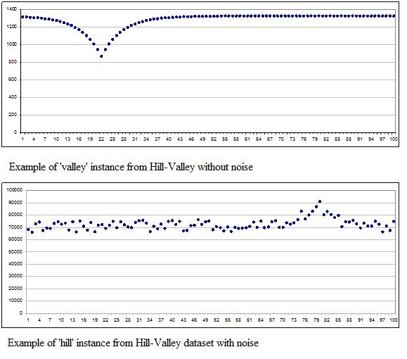
The second issue is how the results from each of the subsets are then combined to obtain an overall result. The RBR is closely related to boosting. Each RBR random bit can be viewed as a weak classifier. Logistic regression is the same as one kind of boosting algorithm named logit-boost. The RBR method boosts those weak bits to form a strong classifier. The RBR is closely related to neural networks. The RBR is equivalent to a single hidden layer neural network and the bits are the hidden units. The most interesting that worth discussing are the ‘hill valley with noise’ and ‘hill valley without noise’ datasets, each record represents 100 points on a two-dimensional graph. When plotted in order (from 1 through 100) as the Y co-ordinate, the points will create either a Hill or a Valley (https://archive.ics.uci.edu/ml/machine-learning-databases/hill-valley/Hill_Valley_visual_examples.jpg). Only RBR and NN performed well (shown in Table 2 of the revised manuscript), and other methods failed. Although these datasets have high dimension and deep interaction between multiple points, with hidden layer neural network, RBR can recognize the complex patterns hidden in these datasets and have better prediction performance. Large number of bits is a conjugate fashion (we call it wide learning) to deep learning. As no back-propagation is required, the learning rule is quite simple, thus is biologically feasible. Biologically, the brain has the capacity to form a huge feature layer (maybe 108 ~ 1010) to approximates functions well.
The third issue is computational cost. The RBR scales well in memory and computation time compared to the SVM due to a fixed number of binary features. The RBR is faster than the random forest or boosting trees due to the light weight nature of the bits.
Conclusions
In conclusion, we can confidently conclude that the RBR is a strong, robust and fast off-the-shelf predictor especially in the big data era.
Abbreviations
- ELM:
-
Extreme learning machine
- GBM:
-
Generalized boosted regression models
- GWAS:
-
Genome-wide association study
- KNN:
-
k nearest neighbor
- Linear:
-
Linear regression
- LR:
-
Logistic regression
- NN:
-
Neural network
- RBR:
-
Random bits regression
- RF:
-
Random forest
- SNP:
-
Single-nucleotide polymorphism
- SVM:
-
Support vector machine
References
Lawrence S, Giles CL, Tsoi AC, Back AD. Face recognition: a convolutional neural-network approach. IEEE Trans Neural Netw. 1997;8(1):98–113.
Oquab M, Bottou L, Laptev I, Sivic J. Learning and transferring mid-level image representations using convolutional neural networks. In: Proceedings of the IEEE conference on computer vision and pattern recognition. 2014. p. 1717–24.
Sarkar M, Leong TY. Application of K-nearest neighbors algorithm on breast cancer diagnosis problem, Proceedings / AMIA Annual Symposium AMIA Symposium. 2000. p. 759–63.
Cortes C, Vapnik V. Support-vector networks. Mach Learn. 1995;20(3):273–97.
Hagan MT, Demuth HB, Beale MH. Neural network design. Boston: Pws Pub; 1996.
Hinton GE, Salakhutdinov RR. Reducing the dimensionality of data with neural networks. Science. 2006;313(5786):504–7.
Huang GB, Zhu QY, Siew CK. Extreme learning machine: a new learning scheme of feedforward neural networks. In: Neural Networks, 2004. Proceedings. 2004 IEEE International Joint Conference on. IEEE. 2004;2:985–90.
Bengio Y, Courville A, Vincent P. Representation learning: a review and new perspectives. IEEE Trans Pattern Anal Mach Intell. 2013;35(8):1798–828.
Breiman L. Random forests. Mach Learn. 2001;45(1):5–32.
Freund Y, Schapire RE. A decision-theoretic generalization of on-line learning and an application to boosting. J Comput Syst Sci. 1997;55(1):119–39.
Bishop CM. Pattern recognition. Machine Learning. 2006;128.
Jain AK, Duin RPW, Mao JC. Statistical pattern recognition: a review. IEEE Trans Pattern Anal Mach Intell. 2000;22(1):4–37.
Muller KR, Mika S, Ratsch G, Tsuda K, Scholkopf B. An introduction to kernel-based learning algorithms. IEEE Trans Neural Netw. 2001;12(2):181–201.
Mohri M, Rostamizadeh A, Talwalkar A. Foundations of machine learning. MIT press, 2012.
Cover TM. Geometrical and statistical properties of systems of linear inequalities with applications in pattern recognition. Ieee Trans Electron. 1965;Ec14(3):326.
Haykin SS, Haykin SS, Haykin SS, Haykin SS. Neural networks and learning machines, vol. 3. Upper Saddle River: Pearson; 2009.
Koh K, Kim S-J, Boyd S. An interior-point method for large-scale l1-regularized logistic regression. J Mach Learn Res. 2007;8(Jul):1519–55.
Bishop CM. Pattern recognition. Mach Learn 2006;128. pp. 137-73.
Hastie T, Tibshirani R, Friedman J. The elements of statistical learning: data mining, inference, and prediction. Secondth ed. 2009.
Bache K, Lichman M. UCI machine learning repository. 2014.
Kaul M, Yang B, Jensen CS. Building accurate 3d spatial networks to enable next generation intelligent transportation systems. In: 2013 IEEE 14th International Conference on Mobile Data Management. IEEE, 2013;1:137–46.
Fanaee-T H, Gama J. Event labeling combining ensemble detectors and background knowledge. Prog Artif Intell. 2013;2(2-3):113–27.
Kibler D, Aha DW, Albert MK. Instance‐based prediction of real‐valued attributes. Comput Intell. 1989;5(2):51–7.
Yeh I-C. Modeling of strength of high-performance concrete using artificial neural networks. Cem Concr Res. 1998;28(12):1797–808.
Cortez P, Morais A. A data mining approach to predict forest fires using meteorological data. In: Proc EPIA 2007. 2007. p. 512–23.
David A, Belsley EK, Roy E. Welsch: regression diagnostics: identifying influential data and sources of collinearity. 2005.
Akbilgic O, Bozdogan H, Balaban ME. A novel hybrid RBF neural networks model as a forecaster. Stat Comput. 2013;24(3):365–75.
Tsanas A, Little MA, McSharry PE, Ramig LO. Accurate telemonitoring of Parkinson’s disease progression by noninvasive speech tests. IEEE Trans Bio-Medical Eng. 2010;57(4):884–93.
Cortez P, Cerdeira A, Almeida F, Matos T, Reis J. Modeling wine preferences by data mining from physicochemical properties. Decis Support Syst. 2009;47(4):547–53.
Gerritsma J, Onnink R, Versluis A. Geometry, resistance and stability of the delft systematic yacht hull series. In: International shipbuilding progress in artificial intelligence. 1981. p. 28.
Bertin-Mahieux T, Ellis DPW, Whitman B, et al. The millon song dataset ISMIR. 2011;2(9):10.
Yeh IC, Yang KJ, Ting TM. Knowledge discovery on RFM model using Bernoulli sequence. Expert Sys Appl. 2009;36(3):5866–71.
Street WN, Wolberg WH, Mangasarian OL. Nuclear feature extraction for breast tumor diagnosis. In: IS&T/SPIE's Symposium on Electronic Imaging: Science and Technology. Int Soc Opt Photonics. 1993:861–70.
Lucas D, Klein R, Tannahill J, Ivanova D, Brandon S, Domyancic D, Zhang Y. Failure analysis of parameter-induced simulation crashes in climate models. Geosci Model Dev. 2013;6(4):1157–71.
Gorman RP, Sejnowski TJ. Analysis of hidden units in a layered network trained to classify sonar targets. Neural Netw. 1988;1(1):75–89.
Gil D, Girela JL, De Juan J, Gomez-Torres MJ, Johnsson M. Predicting seminal quality with artificial intelligence methods. Expert Sys Appl. 2012;39(16):12564–73.
Haberman SJ. Generalized residuals for log-linear models. In: Proceedings of the 9th International Biometrics Conference. 1976. p. 104–22.
Hall M, Frank E, Holmes G, Pfahringer B, Reutemann P, Witten IH. The WEKA data mining software: an update. ACM SIGKDD Explor Newsl. 2009;11(1):10–8.
Ramana BV, Babu MSP, Venkateswarlu NB. A critical comparative study of liver patients from USA and INDIA: an exploratory analysis. Int J Comput Sci Issues. 2012;9(2):506–16.
Sigillito VG, Wing SP, Hutton LV, Baker KB. Classification of radar returns from the ionosphere using neural networks. J Hopkins APL Tech Dig. 1989;10:262–6.
Bock R, Chilingarian A, Gaug M, Hakl F, Hengstebeck T, Jiřina M, Klaschka J, Kotrč E, Savický P, Towers S. Methods for multidimensional event classification: a case study using images from a Cherenkov gamma-ray telescope. Nucl Instrum Methods Phys Res, Sect A. 2004;516(2):511–28.
Mansouri K, Ringsted T, Ballabio D, Todeschini R, Consonni V. Quantitative structure–activity relationship models for ready biodegradability of chemicals. J Chem Inf Model. 2013;53(4):867–78.
Mattern WD, Sommers SC, Kassirer JP. Oliguric acute renal failure in malignant hypertension. Am J Med. 1972;52(2):187–97.
Nair RP, Stuart PE, Nistor I, Hiremagalore R, Chia NV, Jenisch S, Weichenthal M, Abecasis GR, Lim HW, Christophers E. Sequence and haplotype analysis supports HLA-C as the psoriasis susceptibility 1 gene. Am J Hum Genet. 2006;78(5):827–51.
Fang S, Fang X, Xiong M. Psoriasis prediction from genome-wide SNP profiles. BMC Dermatol. 2011;11(1):1.
Guang-Bin H, Qin-Yu Z, Mao KZ, Chee-Kheong S, Saratchandran P, Sundararajan N. Can threshold networks be trained directly? IEEE Trans Circuits Syst II Express Briefs. 2006;53(3):187–91.
Acknowledgement
This research was supported by National Science Foundation of China (31330038) and the 111 Project (B13016). The computations involved in this study were supported by Fudan University High-End Computing Center.
The views expressed in this presentation do not necessarily represent the views of the NIMH, NIH, HHS or the United States Government.
Availability of data and materials
The benchmarked regression and classification datasets were downloaded from the UCI machine learning repository (http://archive.ics.uci.edu/ml/datasets.html). The psoriasis GWAS dataset was obtained from the Genetic Association Information Network (GAIN) database as part of a Collaborative Association Study of psoriasis sponsored by the Foundation for the National Institutes of Health. The psoriasis GWAS dataset were available through dbGaP accession number phs000019.v1.p1. at URL http://dbgap.ncbi.nlm.nih.gov.
Authors’ contributions
YW, YL and LJ conceived the idea, proposed the RBR methods and contributed to writing of the paper. YW, YL and LJ contributed the theoretical analysis. YW also contributed to using C++ to develop the RBR software. YL also contributed to maintaining the RBR software and using R language to generate tables and figures for all simulated and real datasets. MMX contributed to supporting the psoriasis GWAS dataset and revising the paper. YYS contributed to some language corrections and revising the paper. LJ contributed to final revising the paper. All authors read and approved the final manuscript.
Competing interests
The authors declare that they have no competing interests.
Author information
Authors and Affiliations
Corresponding authors
Rights and permissions
Open Access This article is distributed under the terms of the Creative Commons Attribution 4.0 International License (http://creativecommons.org/licenses/by/4.0/), which permits unrestricted use, distribution, and reproduction in any medium, provided you give appropriate credit to the original author(s) and the source, provide a link to the Creative Commons license, and indicate if changes were made. The Creative Commons Public Domain Dedication waiver (http://creativecommons.org/publicdomain/zero/1.0/) applies to the data made available in this article, unless otherwise stated.
About this article

Cite this article
Wang, Y., Li, Y., Xiong, M. et al. Random bits regression: a strong general predictor for big data. Big Data Anal 1, 12 (2016). https://doi.org/10.1186/s41044-016-0010-4
Received:
Accepted:
Published:
DOI: https://doi.org/10.1186/s41044-016-0010-4