
Abstract
Opinion dynamics is an opinion evolution process of a group of agents, where the final opinion distribution tends to three stable states: consensus, polarization, and fragmentation. At present, the opinion dynamics models have been extensively studied in differrent fields. This paper provides a review of opinion dynamics in finance and business, such as, finance, marketing, e-commerce, politics, and group decision making. Furthermore, identified research challenges have been proposed to promote the future research of this topic.
Introduction
Opinion dynamics is the process of studying the evolution of opinions through the social interaction between a group of agents. French and John (1956) first proposed the basic model of opinion dynamics. In last decades, a series of opinion dynamics models with different opinion evolution rules have been proposed, and they can be divided into two categories based on discrete and continuous opinion forms: (1) Discrete opinion models, this type of model is based on physics, such as Sznajd model (Sznajd-Weron and Sznajd 2000), voter model (Clifford and Sudbury 1973; Durrett et al. 2012), majority rule model (Galam 1986, 2002); (2) Continuous opinion models, this kind of model is established mathematically, such as FJ model (Friedkin and Johnsen 1990), DeGroot model (Degroot 1974), DW model (Deffuant et al. 2000; Weisbuch et al. 2002), HK model (Hegselmann and Krause 2002), continuous opinions and discrete actions (CODA) model (Martins 2008). With deeper research on opinion dynamics, some other classic models have been employed in this field, for example, the Ising model (Ising 1925; Glauber 1963; Bianconi 2002).
In opinion dynamics, the final state of opinion evolution tends to three stable states: consensus, polarization, and fragmentation. And the opinion dynamics models usually include three basic elements: opinion expression formats, opinion evolution rules, and opinion dynamics environments. Based on these features, the research on opinion dynamics can improve the understanding of some crucial phenomena in finance and business. There are studies to apply opinion dynamics to many aspects of this field, such as, marketing (Martins et al. 2009; Luo et al. 2014), finance (Kaizoji 2000; Johansen et al. 2000; Bornholdt 2001; Kaizoji et al. 2002), e-commerce (Wan et al. 2018; Zhao et al. 2018b), politics (Bernardes et al. 2001; Stauffer 2002a; Galam 2004), and group decision making (GDM) (Dong et al. 2020; Zha et al. 2019, 2020). Dong et al. (2018b) reviewed the opinion dynamics models within different environments. However, there is no literature review so far to analyze the application of opinion dynamics in finance and business. To this end, this paper provides a clear review of the application of opinion dynamics in finance and business. Moreover, from the insights gained from previous research, we analyze the challenges faced by future research to promote the research of this topic.
The rest of this paper is organized as follows. “Opinion dynamics models and social networks” section introduces the framework and some basic models of opinion dynamics. “Applications of opinion dynamics models in finance” section reviews the application of opinion dynamics in finance and business. Next, “Applications of opinion dynamics models in business” section presents the research challenges of this topic. Finally, the conclusions are drawn in “Summary, critical discussions and new directions” section.
Opinion dynamics models and social networks
Opinion dynamics is a process of individual opinion evolution, in which the interactive agents in the group constantly update their opinions on the same issue based on the evolution rules, and the opinions are stable at the final stage, forming a consensus, polarization, or fragmentation opinion distribution. As described before, the opinion dynamics are divided into two types: Continuous and discrete opinion models. We will introduce some basic models of these two types in “Continuous opinion models” and “Discrete opinion models” sections. A social network can be thought of as a connection between a group of agents who participate in and share various information for the purpose of friendship, marketing or business exchange. Some representative networks are introduced in “Social networks” section.
Continuous opinion models
-
(1)
DeGroot model
In opinion dynamics, the DeGroot model (DeGroot 1974) is considered as the classical model in general. DeGroot (1974) explicitly describes the process which leads to the consensus and specifies the weights that are to be used in Stone (1961). Let \(A = \{ a_{1} ,a_{2} , \ldots ,a_{m} \}\) be the set of agents, and \(o_{i}^{t} \in R\) be the opinion of agent \(a_{i}\) at round \(t\). Assume that \(w_{ij}\) is the weight agent \(a_{i}\) assigns to agent \(a_{j}\), where \(w_{ij} \ge 0\) and \(\sum\nolimits_{j = 1}^{m} {w_{ij} } = 1\). Then, the evolution rule of agent \(a_{i}\) will be:
which equals to:
where \(W = (w_{ij} )_{m \times m}\) is constant and \(O^{t} = (o_{1}^{t} ,o_{2}^{t} , \cdots ,o_{m}^{t} )^{T} \in R^{m}\). DeGroot (1974) believed if there is a \(t\) such that every element in at least one column of the matrix \(W^{t}\) is positive, then a consensus can be reached, and the consensus opinion is a linear combination of the agents' initial opinions.
-
(2)
Bounded confidence model
The bounded confidence (BC) model is an extended study of the DeGroot model, and the weight in Eq. (1) changes with time or opinion. The BC model is based on the following idea: when the difference of opinions between two agents is lower than a given threshold, they will interact, otherwise they will not even bother to discuss. Let \(A = \{ a_{1} ,a_{2} , \ldots ,a_{m} \}\) be the same as before. Let \(o_{i}^{t}\) be the opinion of the agent \(a_{i}\) at round \(t\), which often takes the value from \([0,1]\). Let \(\varepsilon\) be the bounded confidence level, and the BC model will be homogeneous with the \(\varepsilon\) values be the same for all agents; otherwise, it will be heterogeneous. The BC model includes two essential models: the DW model (Deffuant et al. 2000; Weisbuch et al. 2002), and the HK model (Hegselmann and Krause 2002, 2005). In the following, we introduce these two models.
-
(a)
DW model
Two agents are randomly chosen from set \(A\), and they will determine whether to interact according to the bounded confidence. If \(|o_{i}^{t} - o_{j}^{t} | > \varepsilon\), the agents \(a_{i}\) and \(a_{j}\) will think that opinions are too far apart to interact; otherwise, the evolution rule will be:
where \(\mu \in [0,{0}{\text{.5}}]\) is the convergence parameter. Depending on the parameters \(\varepsilon\) and \(\mu\), a consensus, polarization, or fragmentation opinion distribution will be obtained in the DW model.
(b) HK model.
Let \(w_{ij}^{t}\) be the weight that agent \(a_{i}\) gives to \(a_{j}\) at round \(t\), which is described as:
where \(S_{i}^{t} = \{ a_{j} ||o_{i}^{t} - o_{j}^{t} | \le \varepsilon \}\) is the confidence set of agent \(a_{i}\), and \({|} \cdot {|}\) denotes the absolute value of a real number and the number of elements for a finite set.
Then, the opinion evolution rule is as follows:
If there exists an ordering \(o_{i1} \le o_{i2} \le \cdots \le o_{im}\) such that two adjacent opinions are within the bounded confidence level \(\varepsilon\), then the opinion profile \(O = o_{1} ,o_{2} , \ldots ,o_{m}\) is called an ε-profile. Hegselmann and Krause (2002) argue that the opinion profile will be an ε-profile for all times if a consensus is reached for an initial profile. Moreover, two agents will remain separated forever if they split at some time.
Discrete opinion models
The discrete opinion models mostly use binary opinions for research at the beginning. As the research deepens, some extended models use multiple opinions to study more complex situations. Some basic models will be introduced below.
-
(1)
Voter model
The voter model (Clifford and Sudbury 1973) is a discrete opinion dynamics model with all agents been widely placed in a two-dimensional lattice. Let \(A = \{ a_{1} ,a_{2} , \ldots ,a_{m} \}\) be the set of agents as before, and \(o_{i}^{t}\) be a binary opinion of agent \(a_{i}\) at round \(t\), where \(o_{i}^{t} = 1\) or \(o_{i}^{t} = - 1\). The agent will randomly select an agent among the four neighbors and follow his/her opinion. Without loss of generality, agents \(a_{j}\) is assumed to be the selected neighbor. Then, the opinion \(o_{i}^{t + 1}\) of agent \(a_{i}\) will be \(o_{j}^{t}\), i.e., \(o_{i}^{t + 1} = o_{j}^{t}\). The voter model leads to two possible consensus states, and the probability of opinions to reach a consensus is determined by the initial distribution of opinions. Furthermore, a consensus is reached only for dimension \(d \le 2\) in an infinite system (Cox 1989).
-
(2)
Snajzd model
The Snajzd model is also a discrete opinion dynamics model for the one-dimensional case (Sznajd-Weron and Sznajd 2000), which is based on the characteristic of "United we Stand, Divided we Fall". And the opinion \(o_{i}^{t} = \pm 1\) is a binary opinion of agent \(a_{i}\) at round \(t\). Then, the opinions evolve according to the following rules:
-
(a)
In each round a pair of agents \(a_{i}\) and \(a_{i + 1}\) is selected to influence their nearest neighbors, i.e. the agents \(a_{i - 1}\) and \(a_{i + 2}\).
-
(b)
If \(o_{i}^{t} = o_{i + 1}^{t}\), then \(o_{i - 1}^{t + 1} = o_{i + 2}^{t + 1} = o_{i}^{t}\).
-
(c)
If \(o_{i}^{t} = - o_{i + 1}^{t}\), then \(o_{i - 1}^{t + 1} = o_{i + 1}^{t}\) and \(o_{i + 2}^{t + 1} = o_{i}^{t}\).
A different version of rule (c) proposed later is now more widely used and will be introduced in “Application of basic models” section. The difference from the voter or Ising model is the outflow of information. And, two types of stable states are always reached in this model: complete consensus or stalemate.
-
(3)
Ising model
Ising model is a well-known model in physics to explain the phase transition of ferromagnetic materials (Ising 1925). In opinion dynamics, it has been well studied over last decades to model the social interactions (Glauber 1963; Binder 1981; Harris 2001; Herrero 2002; Bianconi 2002). The energy \(E\) of interaction between two magnetic particles in Ising’s original work corresponds to the degree of conflict of opinions between two agents in opinion dynamics, as shown below
where \(o_{i}\) denotes the ith particle’s intrinsic spin and constant \(J\) is an energy coupling constant. And \(o_{i} { = + 1}\) or − 1 correspond to a up state and a down state respectively. In opinion dynamics, \(o_{i}\) indicates a binary opinion of agent \(a_{i}\) and \(J\) represents the interaction strengths among agents. When the spins of two interacting particles are parallel, the energy of the interaction is minimal, that is, the degree of conflict of opinions between two agents will be minimal when they have the same opinion. Furthermore, the interaction energy also exists between the magnetic particles and the external magnetic field \(H\), that is,
where \(H\) represents the external information in opinion dynamics (e.g. media promotion). This energy will be minimized when the particle’s spin has the same value as the external field. The external field models the media promotion effect of opinions. If the opinions of agents are consistent with the media, the lower the energy and therefore the more harmonious. Then, the total energy of interaction can be described as
Social networks
Social network can be simply thought of as the structure of social relations. Social network can refer to not only the network between people, but also the network between organizations and organizations, even the network of relations between cities and cities, and the network of relations between countries and countries. The network approach greatly contributes to our understanding of complex system structure, trust propagation and influence, etc. In opinion dynamics, social network mainly refers to the network between agents, which can be defined by a graph with nodes representing agents and edges indicating relationships between agents. Three representative complex networks are introduced below:
Erdős–Rényi (ER) random network: The "random" of a random network is mainly reflected in the distribution of edges. A random network actually connects the given nodes randomly. The ER model means that in a given \(m\) nodes, it is specified that every two nodes are connected with a probability of \(p\) \((0 \le p \le 1)\). The clustering coefficient and average path length of the ER random network are very small, where the first property reflects the coincidence degree of friends between two neighbors, and the second one refers to the average of the shortest path length between any two nodes in a network.
Small-world (SW) network: In this network, most of the nodes are not connected to each other, but most of the nodes can be reached after a few connections. In daily life, sometimes you will find that some people who you think are "far away" from you are actually "close" to you. The SW network is a mathematical description of this phenomenon. Although the SW network has a small average path length, it also has a considerable higher clustering coefficient than the random network.
Scale-free (SF) network: The SF network has serious heterogeneity, and the connection status (degree) between the nodes has a serious uneven distribution: a few nodes in the network have extremely many connections, and most nodes have only a few connections. The nodes with extremely many connections play a leading role in the SF networks. Generally speaking, the scale-free nature is an inherent property that describes the serious uneven distribution of complex systems.
Applications of opinion dynamics models in finance
In this section, we introduce the applications of opinion dynamics from two aspects: Basic model application and extended application.
Application of basic models
The financial market is a very complex system, composed of competing and interacting economic agents with different strategies, motivations and investment horizons (Mitchell and Mulherin 1994; Feng and Seasholes 2005; Hou and Moskowitz 2005; Kaminsky and Schmukler 2007; Tetlock 2007; Diether et al. 2009; Easley et al. 2016). In the financial application, the binary opinion dynamics models are the most common. In this section, we present the application of three binary opinion dynamics models (i.e., the Ising model and the Snazjd model) in financial market. In these studies, the price changes proportional to the difference between demand and supply. An obvious requirement is that more demand than supply will push up the prices, and similarly for the opposite case.
-
(1)
Application of the Ising model
As described before, the Ising model is a well-known model in physics (Ising 1925), which also has attracted a lot of attention in the modeling of financial systems. Table 1 summarizes the applications of the Ising model in financial market. Here we introduce the basic applications of the Ising model or Ising-like model in financial market (Bornholdt 2001; Krawiecki et al. 2002; Sornette and Zhou 2006; Chowdhury and Stauffer 1999).
The Ising model is a model with \(i = 1,2, \ldots ,m\) spins with orientations \(o_{i}^{t} = \pm 1\), corresponding to agent \(a_{i}\) with the actions at round \(t\) in financial market in Bornholdt (2001). And \(o_{i}^{t} = + 1\) is interpreted as a bullish trader \(a_{i}\) who places buy orders at round \(t\), while \(o_{i}^{t} = + 1\) is interpreted as a bearish trader \(a_{i}\) who places sell orders. Assume that \(H_{i}^{t}\) is the local field and \(\beta\) is a responsiveness parameter. And then the evolution rule is described as:
where \(p\) is the probability of opinion evolution. And the local field \(H_{i}^{t}\) is specified by
where \(J_{ij}\) represents the interaction strength (possibly 0) between traders \(a_{i}\) and \(a_{j}\); \(\alpha > 0\) is a global coupling parameter; \(C_{i}^{t}\) is a strategy of trader \(a_{i}\) at round \(t\).
Similar to Bornholdt (2001), \(o_{i}^{t} = \pm 1\) has the same meaning in Krawiecki et al. (2002). And the evolution rule is as follows:
where the local field \(H_{i}^{t}\) is below:
with interaction strength \(J_{ij}^{t}\) changing over time and external field \(h_{i}^{t}\) indicating the effect of environment.
Sornette and Zhou (2006) extended the Ising model and introduced the following evolution rules:
Equation (13) embodies three contributions:
-
(a)
Mutual influences \(\sum\nolimits_{j = 1}^{m} {J_{ij}^{t} E^{t} [o_{j}^{t} ]}\): \(J_{ij}^{t}\) quantifies the interaction strength of the expected decision of trader \(a_{j}\) on trader \(a_{i}\); \(E^{t} [o_{j}^{t} ]\) is the expected decision of trader \(a_{j}\) estimated by trader \(a_{i}\).
-
(b)
External news \(\sigma_{i} G(t)\): \(\sigma_{i}\) is the relative sensitivity of trader \(a_{i}\) to the external news; \(G(t)\) is defined as the influence of the external news on the decision of trader \(a_{i}\).
-
(c)
Idiosyncratic judgements \(\varepsilon_{i}^{t}\): \(\varepsilon_{i}^{t}\) indicates the trait of the decision of trader \(a_{i}\) for the explanation of her personal information.
Chowdhury and Stauffer (1999) proposed an Ising-like stock market model, which includes three states of a trader: \(+ |o_{i} |\) (buy), \(- |o_{i} |\) (sell), and 0 (not to trade). And the evolution rule is below:
-
(a)
A trader picks up the \(+ |o_{i} |\) with probability \(b\), \(- |o_{i} |\) with probability \(b\) and the 0 with probability \(1 - 2b\).
-
(b)
Then the trader \(a_{i}\) changes into the state picked up with probability \(e^{{ - \Delta E_{i} /(k_{B} T)}}\), where \(T\) represents the fictitious temperature, and \(\Delta E\) is the change of disagreement connected with this transition. Let \(h_{i}\) be the individual bias of the trader \(a_{i}\). And the disagreement functions of noise trader and fundamentalist trader are defined as Eqs. (14) and (15), respectively.
$$E_{i} = - o_{i} H_{i}$$(14)$$E_{i} = - o_{i} (H_{i} + b_{i} )$$(15)with the local field \(H_{i}\):
$$H_{i} = \sum\limits_{j = 1,j \ne i}^{m} {J_{ij} o_{j} }$$(16)where \(J_{ij}\) is the interaction strength between traders \(a_{i}\) and \(a_{j}\)
.
-
(2)
Application of the Sznajd model
So far, the possible financial application of the Sznajd model has not received much attention. Sznajd-Weron and Weron (2002) studied the price formation in a financial market based on the one-dimensional Sznajd model. Let \(A = \{ a_{1} ,a_{2} , \ldots ,a_{m} \}\) be the set of agents. In the Sznajd model, \(o_{i}^{t}\) is a binary opinion of agent \(a_{i}\) at round \(t\), here \(o_{i}^{t}\) is defined as the attitude of market participant \(a_{i}\). And \(o_{i}^{t} = + 1\) has the same meaning as the application of the Ising model in “Applications of opinion dynamics models in finance” section (1). Then, the opinion evolution represents the dynamic state of the trader, and the dynamic rule is as shown below:
-
(a)
In each round, a pair of traders \(a_{i}\) and \(a_{i + 1}\) is chosen to affect their neighbors, i.e. the traders \(a_{i - 1}\) and \(a_{i + 2}\).
-
(b)
If \(o_{i}^{t} o_{i + 1}^{t} = 1\), that is, traders \(a_{i}\) and \(a_{i + 1}\) have the same state, then traders \(a_{i - 1}\) and \(a_{i + 2}\) follow the state of the traders \(a_{i}\) and \(a_{i + 1}\), that is \(o_{i - 1}^{t + 1} = o_{i + 2}^{t + 1} = o_{i}^{t} = o_{i + 1}^{t}\). The reason for this dynamic rule is that many market participants are trend followers who place orders according to the opinions of local gurus.
-
(c)
If \(o_{i}^{t} o_{i + 1}^{t} = - 1\), then traders \(a_{i - 1}\) and \(a_{i + 2}\) randomly choose to buy or sell, namely, \(o_{i - 1}^{t + 1} ,o_{i + 2}^{t + 1} = - 1{\text{ or } + \text{ 1}}\) at random. This dynamic rule incorporates the fact that the absence of a local guru, i.e., traders \(a_{i}\) and \(a_{i + 1}\) are in different state, will cause the trend followers in market to act randomly.
-
(d)
In financial market, trend followers are not the only remaining market participants (Bak et al. 1997). Some rational traders also exist, and they know the system better and have strategies. For simplicity, Sznajd-Weron and Weron (2002) introduced one rational trader in the proposed model, who known exactly the difference between demand and supply in the current market. He/she places buy orders when there is more demand than supply, and vice versa. Sznajd-Weron and Weron (2002) argued that \(p_{t} = {1 \mathord{\left/ {\vphantom {1 m}} \right. \kern-\nulldelimiterspace} m}\sum\nolimits_{i = 1}^{m} {o_{i}^{t} }\) is the price at round \(t\). Then, this rule is that the rational trader \(a_{k}\) will buy (i.e., \(o_{k}^{t} = + 1\)) at round \(t\) with probability \(|p_{t} |\) when \(p_{t} < 0\), and sell (i.e., \(o_{k}^{t} = - 1\)) with probability \(|p_{t} |\) when \(p_{t} > 0\).
Sabatelli and Richmond (2004) proposed a model of trading orders based on a Sznajd-like interaction, and this study showed how the proposed model is compatible with some of the main statistical characteristics observed in asset volumes in financial markets.
-
(2)
Application of the voter model
Krause and Bornholdt (2012) used a two-dimensional voter model with a tunable social temperature to study the opinion evolution process among traders. In this model, agent \(a_{i}\) adapts the opinion \(o_{i}^{t} { = } \pm {1}\) (buy or sell) based on his/her nearest neighbors. Let \(u_{i}\) be the number of agreeing neighbors of agent \(a_{i}\). Then, the opinion evolution is described with the flip probabilities \(p_{{u \to 4{ - }u}}\), where \(p_{{u \to 4{ - }u}} { + }p_{{{4 - }u \to u}} { = 1}\). With suppressed voluntary isolation this model argues that \(p_{{{2} \to {2}}} { = 1/2}\), \(p_{{{0} \to 4}} { = 1}\), and \(p_{{{4} \to {0}}} { = 0}\). Based on the inverse temperature \(\beta { = 1/}T\), the remaining probability of join local minorities \(p_{{{3} \to {1}}}\) is set as follows:
The social temperature \(T\) can be regarded as the market temperature, because it affects the uncertainty of all agents' investment strategies. For low temperatures the persuasiveness of local groups of agents will be increased (\(p_{1 \to 3} > 3p_{{{3} \to {1}}}\)). Meanwhile, the persuasiveness of local majorities will be suppressed for higher temperatures.
There are other applications of voter and voter-like models in financial markets. For example, Zubillaga et al. (2019) studied the financial market with the majority-vote model, and includes three states, i.e., buy, sell or remain inactive; Vilela et al. (2019) also applied the majority-vote model to research the financial market; Wang et al. (2019) studied the complex and composite entropy fluctuation behaviors through a voter interacting system.
The basic models follow the statistical physics-based models and are traditionally designed to capture several regulatory real-life phenomena. These opinion dynamics studies use different opinion evolution rules to model the microscopic dynamics among agents, meanwhile, study the trends, bubbles and crashes of the financial market from the macroscopic level. And the basic binary opinion dynamics models provides tools and methods to study the phase transition, metastable phase and structured lattice critical point.
Extension application
The application of the opinion dynamics models in financial research have been studied from many aspects. Here we mainly introduce the following two extension applications.
-
(1)
Kinetic models of opinion formation
The basic opinion dynamics models study the financial market by the methods and tools from classical statistical mechanics, where the complex behaviors arise from relatively simple interaction rules. The mathematical framework that characterizes financial markets is another research line (Maldarella and Pareschi 2012; Cordoni and Di Persio 2014). The kinetic models of opinion formation consider opinion dynamics analysis from the point of view of mathematical framework involving both opinion exchange between agents and information diffusion (Toscani 2006). Compared to the basic opinion dynamics models with the discrete opinion and time, the kinetic models of opinion formation provide tools to analyze microscopic dynamics of each trading agent in financial market using the continuous opinion and time. Furthermore, in contrast to the basic opinion dynamic models that usually only study behavior empirically through computer simulation, the kinetic models based on partial differential equations allow us to obtain analytical general information about the model and its asymptotic behavior. Maldarella and Pareschi (2012) studied the kinetic models for socio-economic dynamics of speculative markets characterized by two different market strategies, chartists and fundamentalists, similar to Lux and Marchesi model (Lux and Marchesi 1999, 2000). This study uses the kinetic system coupling a description for the price formation mechanism and the propensity of investment of chartists.
-
(2)
Data-driven opinion dynamics models
Data-driven opinion dynamics models are study the opinion evolution from a more computational point of view. Das et al. (2014) observed three distinct types of opinion evolution processes derived from stubbornness, compromise, and biased conformity in the carefully crafted experiments and proposed a biased-voter model based on these observations. De et al. (2014) proposed a linear influence opinion dynamics model, where the edge influence strengths are estimated, not assumed, from an observed series of opinions of agents using the projected gradient descent algorithm. De et al. (2016) proposed a probabilistic modeling framework of opinion dynamics with efficient model simulation and parameter estimation from historical fine grained event data, where opinions over time are represented by means of marked jump diffusion stochastic differential equations. To extend the contribution in De et al. (2016), t, Kulkarni et al. (2017) applied a network-guided recurrent neural network architecture to capture a generic form of nonlinear dependencies between the social network and the past events to model the nonlinear opinion dynamics in social networks. Di Persio and Honchar (2016) argue that even if only training on plain time series data, neural networks can predict the movements of financial time series. Although data-driven opinion dynamics models have not been studied in the financial market environment, all the studies described above provide a good research foundation. Using machine learning to study the microscopic dynamics of the trading agents and the collective behaviors will be of great help in financial forecasting.
Applications of opinion dynamics models in business
In this section, we introduce the applications of opinion dynamics in marketing, e-commerce, politics and decision making.
Marketing
The use of opinion dynamics models in marketing focuses on modeling two influential factors: advertising and word-of-mouth recommendations from friends. Specifically, we introduce the use of some basic opinion dynamics models in marketing below.
-
(1)
Application of the CODA model
Martins et al. (2009) and Luo et al. (2014) studied the dynamics of customers opinions affected by advertising and word of mouth using the CODA model. When using the CODA model in marketing, two choices are often considered, i.e., adoption and non-adoption of a new product. Let \(o_{i}^{t}\) (continuous variable) be the inner opinion of agent \(a_{i}\) associated with a product or service at round \(t\). Let \(s_{i}\) be the binary choices in regards to agent \(a_{i}\). If agent \(a_{i}\) chooses to adopt the product or service, then \(s_{i} = + 1\); otherwise, \(s_{i} = 0\). And the relation between the action \(s_{i}\) and the opinion \(o_{i}\) of agent \(a_{i}\) can be:
Luo et al. (2014) studied both influential factors, and then, the opinion evolution of agent \(a_{i}\) can be described as:
where \(F_{i}^{t}\) indicates the influence that agent \(a_{i}\) affected by his/her friends, and is related to the actions of his/her friends; \(AD_{i}^{t}\) represents the influence of the advertising on agent \(a_{i}\).
-
(2)
Application of the Sznajd model
Schulze (2003) and Sznajd-Weron and Weron (2003) studied that how strong an advertising must be to support one of the two products to conquer the market depending on the Sznajd model in a two-dimensional setup. Assuming that \(o_{i}^{t}\) is the binary opinion of agent \(a_{i}\) of the Sznajd model, it corresponds to the situation where the customer \(a_{i}\) supports product \(x_{A}\) or \(x_{B}\). Then, the opinion evolution rule is described as follows (Sznajd-Weron and Weron 2003):
-
(a)
Randomly select an agent (that is, a customer *), and then form a panel (dark blue site) with his/her three neighbors. This panel can affect the eight nearest neighbors (light blue site), as shown in Fig. 1.
Fig. 1 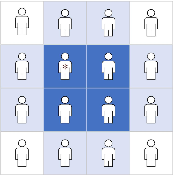
Rules affecting neighbors
-
(b)
If the four agents in a panel support the same product, all eight neighbors will be affected to support the same product.
-
(c)
If one of the agents in a panel supports the product opposite to the other three agents, the neighbors will support the product supported by the majority with probability 3/4 and will be responsive to the advertising with probability 1/4.
-
(d)
In the case of two agents in the panel supporting product A and two agents supporting product B, any neighbor will not be persuaded by the panel, but will respond to advertising.

-
(3)
Application of the BC model
Salehi and Taghiyareh (2014) studied the opinion prediction of agents based on the BC model to identify suitable products and customers and determine the correct marketing strategy. Suppose that \(o_{ik}^{t}\) is the opinion of agent \(a_{i}\) about product \(x_{k}\), where \(o_{ik}^{t} \in [ - 1,1]\), and opinions of agents can be divided into three categories, namely, positive, negative and don't care. Let \(d\) be the bounded confidence. Similar to Pazzani (1999), two agents \(a_{i}\) and \(a_{j}\) are selected to interact. If \(|o_{ik}^{t} - o_{jk}^{t} | < d\), the opinion evolution will be:
where \(\mu\) is a parameter about the degree of trust \(T_{ij}\) between the selected two agents, i.e., \(\mu { = }T_{ij}\). And \(T_{ij}\) is a dynamic value according to the opinions of agents.
Applying this method, a prediction of opinions and some clusters for each product will be obtained. Salehi and Taghiyareh (2014) argued that these results can be used to create management reports and support managers in choosing the right products to produce, and choosing the right customers or communities to promote different products.
Moreover, there are other studies using the opinion dynamics models research marketing. Taghiyareh's team studied this issue from different aspects (Nazemian and Taghiyareh 2012; Salehi and Taghiyareh 2014; Vadoodparast et al. 2014; Vadoodparast and Taghiyareh 2015; Salehi and Taghiyareh 2019). Günther et al. (2011) proposed an agent-based simulation method to support managers in marketing activities, and illustrated the method by taking the new product diffusion of a novel biomass fuel as an example. Chasparis and Shamma (2012) studied the issue of obtaining the optimal marketing policies for the diffusion of innovations based on the FJ model. Maghami and Sukthankar (2012, 2013) studied the influence of advertising in marketing using independent cascade model. Bimpikis et al. (2016) examines a game-theoretic model of competition between firms with the optimal targeted advertising strategies based on the binary voter model. Varma et al. (2017) analyzed the competition between two firms to capture a larger market share based on the DeGroot model. Table 2 summarizes the applications of opinion dynamics in marketing.
E-commerce
In this section, the BC model is a useful tool to study the opinion evolution of consumer in the e-commerce environment. Online consumer reviews and opinion leaders are two important factors that affect consumers' opinions on products. Wan et al. (2018) and Zhao et al. (2018b) used the BC model to study the fluence of the two factors in the e-commerce environment, respectively. Here we mainly introduce their use of the BC model in the e-commerce environment.
Wan et al. (2018) argued that a consumer will retain his/her opinion, but change it slightly based on the average of all other trustworthy reviews. Let \(\mu\) be the convergence parameter which indicates consumers’ level of trust in reviewers. Then, the evolution rule on an e-commerce platform is as follows:
where the trustworthy reviews are selected by:
where \(\varepsilon\) is the bounded confidence.
Zhao et al. (2018b) studied the influence power of opinion leaders in e-commerce networks, and divided the consumers into two groups: opinion leaders and followers. Zhao et al. (2018b) considered a social network composed of \(m\) agents, including \(m_{1}\) followers, \(m_{2}\) leaders with a positive target opinion, \(m_{2}\) leaders with a negative target opinion, and \(m_{1} + m_{2} + m_{3} = m\). Then, the updating rule of followers is below:
The updating rule of leaders with a positive target opinion is below:
The updating rule of leaders with a negative target opinion is below:
where
and \(\varepsilon_{i}\) represents the bounded confidence of consumer \(a_{i}\); \(m_{i}^{F,t} = \sum\nolimits_{j = 1}^{{m_{1} }} {A_{ij}^{t} }\) is the number of neighbors of follower \(a_{i}\); \(m_{i}^{P,t} = \sum\nolimits_{{j = 1 + m_{1} }}^{{m_{2} }} {A_{ij}^{t} }\) and \(m_{i}^{N,t} = \sum\nolimits_{{j = 1 + m_{1} + m_{2} }}^{m} {A_{ij}^{t} }\) are the total number of opinion leaders of agent \(a_{i}\) who is from the positive and negative leader subgroups, respectively; \(\alpha_{i}\), \(\beta_{i}\), and \(1 - \alpha_{i} - \beta_{i}\) are the trust degrees; \(d \in [0,1]\) is the positive target opinion value; \(g \in [ - 1,0]\) is the negative target opinion value; and \(w_{i}\) and \(z_{i}\) are the influence weights. It is worth mentioning that \(A_{ij}^{t}\) does not directly evolve over time, but depends on the value of \(o_{i}^{t}\).
Applications of opinion dynamics models in GDM
GDM is an important research content of business, for example, the selection of suppliers is a matter of GDM. In the process of supplier selection, multiple members from the company constitute a decision-making committee. The decision-making committee needs to work together to select a suitable supplier. In GDM, consensus reaching is an important research direction (Li et al. 2019; Xu et al. 2020; Zhang et al. 2020). Dong et al. (2018a) summarized the use of opinion dynamics models in this field, and also in Ureña et al. (2019a). Here we mainly summarize the research results of the past two years to supplement these two literatures, as shown in Table 3.
In a rational and democratic society, "voting" is one of the two basic methods of GDM, usually used to make political decisions. For example, the decision-making of the UN Security Council is a matter of group decision-making. When the Security Council makes decisions, the five permanent members form a group, and they need to negotiate and discuss together to find a solution to a problem. The opinion dynamics models have been widely used in "political" decisions. Most of the models are the discrete opinion dynamics models, such as Sznajd model (González et al. 2004; Sznajd-Weron 2005), voter model (Yildiz et al. 2013; Pérez et al. 2015); majority rule model (Galam 1999, 2004, 2007; Galam and Jacobs 2007). It is worth to notice that the minority opinion spreading is important for the voting result, which explains why an initially minority opinion can become a majority in the long run (Galam 2002; Stauffer 2002b; Tessone et al. 2004; Kułakowski and Nawojczyk 2008). A summary of the applications of the opinion dynamics models in politics is shown in Table 4. In this section, we mainly introduce the use of the voter and majority rule models in politics because of the application details of other discrete models has been introduced in the previous sections.
-
(1)
Application of the voter model
Yildiz et al. (2013) studied the voter model in a social network with Stubborn voters, and the basic use of the voter model in politics is described in the following. Let \(G(A,E)\) be a directed graph to represent the social network, where \(A = \{ a_{1} ,a_{2} , \ldots ,a_{m} \}\) is the set of voters and \(E\) is the set of edges representing the relationships among the voters. \((a_{i} ,a_{j} ) \in E\) is an edge from voter \(a_{i}\) to voter \(a_{j}\), and the set \(N_{i} = \{ a_{j} |(a_{i} ,a_{j} ) \in E\}\) is defined as the neighbor set of voter \(a_{i} \in A\). Assume that \(o_{i}^{t} \in \{ 0,1\}\) is the voting status of agent \(a_{i}\) at round \(t\) representing the selection of agent \(a_{i}\) among two candidates in the election. Then, the evolution rule is as follows:
-
(a)
One of the neighbors of the agent \(a_{i}\) is randomly and uniformly selected, i.e., agent \(a_{j}\).
-
(b)
Then, the voting status of agent \(a_{i}\) at round \(t + 1\) will be:
$$o_{i}^{t + 1} = o_{j}^{t}$$(27)
-
(2)
Application of the majority rule model
Galam (1999) studied the majority rule model in hierarchical structures, and the basic use of the majority rule model in this paper is described as follows. Let \(A = \{ a_{1} ,a_{2} , \ldots ,a_{m} \}\) and \(o_{i}^{t} \in \{ 0,1\}\) be the same as before. Then, the evolution rule is below:
-
(a)
Randomly select \(r\) voters to form a cell.
-
(b)
In each cell, the voting status of agent \(a_{k}\) at round \(t + 1\) will be:
$$o_{k}^{t + 1} = \left\{ {\begin{array}{*{20}c} {\begin{array}{*{20}c} 1 \\ {o_{k}^{t} } \\ 0 \\ \end{array} } & {\begin{array}{*{20}l} {if{{ \, \sum\nolimits_{i = 1}^{r} {o_{i}^{t} } } \mathord{\left/ {\vphantom {{ \, \sum\nolimits_{i = 1}^{r} {o_{i}^{t} } } r}} \right. \kern-\nulldelimiterspace} r} > 0.5} \hfill \\ {if{{ \, \sum\nolimits_{i = 1}^{r} {o_{i}^{t} } } \mathord{\left/ {\vphantom {{ \, \sum\nolimits_{i = 1}^{r} {o_{i}^{t} } } r}} \right. \kern-\nulldelimiterspace} r} = 0.5} \hfill \\ {otherwise} \hfill \\ \end{array} } \\ \end{array} } \right.$$(28)
Summary, critical discussions and new directions
Opinion dynamics is a useful tool to model the diffusion and opinion evolution among a group of interactive agents. In opinion dynamics models, there are three key elements in general: opinion expression formats, evolution rules and opinion evolution environments. Due to different opinion expression formats, the opinion dynamics models with different evolution rules can be divided into continuous and discrete categories. Opinion dynamics mainly studies the mutual influence of opinions among agents by exchanging information and the evolution of opinion to form a consensus, fragmentation or polarization phenomenon. Based on this feature, the opinion dynamics models have been applied to the fields of finance and business with different opinion evolution environments, such as marketing, finance, e-commerce, politics, and GDM. Although opinion dynamics models have been studied in many aspects in finance and business, which can help us understand the rules and important factors of opinion evolution in different scenarios, there are still some limitations that need to be paid attention to:
-
1
Most opinion dynamics researches mainly follows the methods and tools of the statistical physics-based models, and the data sets used usually employ random data in the simulation (Dong et al. 2016, 2017, 2018b; Ding et al 2017, 2019). Few studies (Das et al. 2014; De et al. 2014, 2016; Kulkarni et al. 2017) have used real data to drive opinion dynamics processes.
-
2
Although the opinion dynamics model has been studied in many aspects in the finance and business, it is still focused on the characteristics of the opinion dynamics model. The combination with the characteristics of its application field is still insufficient.
-
3
In opinion dynamics, there are mainly two kinds of opinion expression forms, discrete and continuous, which are mainly expressed in the form of numbers (Martins et al. 2009; Maghami and Sukthankar 2012, 2013; Luo et al. 2014; Liang et al. 2016). In the actual opinion expression, the linguistic term is very common, for example, word-of-mouth, and advertising.
-
4
Network is a powerful method for modeling and studying various complex phenomena, and collective phenomena emerges from the interactions between dynamical processes in multiplex networks (Nicosia et al. 2017). However, in the applications, the social network generally is assumed to be static during the interaction (Kaizoji 2000; Sznajd-Weron and Weron 2003; Sznajd-Weron 2005; Varma et al. 2018).
Thus, future research on this topic can follow the directions below:
-
1
Using real data to study opinion dynamics and developing a real data driven opinion dynamics model will be an interesting topic. Meanwhile, studying data-driven opinion dynamics models in finance and business will be interesting.
-
2
It would be interesting to consider opinion dynamics from the point of view of mathematical finance works more oriented to the “continuous time” treatment of technical topics.
-
3
There will be cost/resource constraints associated with opinion changes in product selection, it will be an interesting research direction to use the opinion dynamics models to study marketing strategy with minimum cost.
-
4
The Ising model is a basic model to simulate the stock market (Kaizoji 2000; Johansen et al. 2000; Bornholdt 2001; Kaizoji et al. 2002; Eckrot et al 2016; Takaishi 2017), and the strategies of trader's buy and sale are diverse. Therefore, it would be interesting to use the Ising model to study financial market from the perspective of individual personalization.
-
5
In marketing, word-of-mouth and advertising are presented in the form of linguistic term. It is necessary to study the opinion dynamics of agents with different forms of opinion expression, especially the interaction using linguistic term. And this will make research on the effects of word-of-mouth and advertising more realistic in marketing.
-
6
Complex networks [e.g. ER random network (Erdős and Rényi 1960), SW network (Newman and Watts 1999), and SF network (Barabasi and Albert 1999)] have been extensively studied in opinion dynamics. However, research on the impact of the dynamic network in the existing literature is still insufficient. The Hopfield neural network model can express homogenous attraction and heterogeneous repulsion (Li and Tang 2013). Therefore, using this model to study group dynamics such as global differentiation and local convergence in financial markets is a promising research direction.
-
7
The application of opinion evolution in GDM and e-commerce is beginning to be recognized (Dong et al. 2017, 2018a, 2018b, 2020; Wan et al. 2018; Zhao et al. 2016, 2018a, b; Liang et al. 2020), and it is still necessary to further develop the theoretical basis for in-depth interdisciplinary integration research.
Conclusions
This paper reviews the application of the opinion dynamics models in finance and business. Firstly, we introduce some basic opinion dynamics models, including the DeGroot model, the BC model, the Snajzd model, and the voter model. Then, we review the use of opinion dynamics in different aspects of finance and business, including marketing, finance, e-commerce, politics, and group decision making. In the end, we note some limitations of the existing studies that need to be paid attention to and suggest several new directions for future research.
Availability of data and materials
Not applicable.
Abbreviations
- CODA:
-
Continuous opinions and discrete actions
- BC:
-
Bounded confidence
- GDM:
-
Group decision making
- ER:
-
Erdős–Rényi
- SW:
-
Small-world
- SF:
-
Scale-free
References
Bak P, Paczuski M, Shubik M (1997) Price variations in a stock market with many agents. Phys A 246(3–4):430–453
Barabasi AL, Albert R (1999) Emergence of scaling in random networks. Science 286(5439):509–512
Ben-Naim E (2005) Opinion dynamics: rise and fall of political parties. EPL Europhys Lett 69(5):671
Bernardes AT, Costa UMS, Araujo AD, Tauffer D (2001) Damage spreading, coarsenig oarsening dynamics and distbution of political voets in sznajd model on square lattice. Int J Mod Phys C 12(2):159–167
Bernardes AT, Stauffer D, Kertész J (2002) Election results and the Sznajd model on Barabasi network. Eur Phys J B 25:123–127
Bianconi B (2002) Mean field solution of the Ising model on a Barabasi-Albert network. Phys Lett A 303:166
Bimpikis K, Ozdaglar A, Yildiz E (2016) Competitive targeted advertising over networks. Oper Res 64(3):705–720
Binder K (1981) Finite size scaling analysis of Ising model block distribution functions. Eur Phys J A 2(2):79–100
Biswa S, Sen P (2017) Critical noise can make the minority candidate win: the U.S. presidential election cases. Phys Rev E 96:032303
Bornholdt S (2001) Expectation bubbles in a spin model of markets: intermittency from frustration across scales. Int J Mod Phys C 12(05):667–674
Bornholdt S, Wagner F (2002) Stability of money: phase transitions in an Ising economics. Phys A 316:453–468
Chasparis G, Shamma JS (2012) Control of preferences in social networks. Abstract from 4th World Congress of the Game Theory Society. Istanbul, Turkey
Chen X, Ding ZG, Dong YC, Liang HM (2020) Managing consensus with minimum adjustments in group decision making with opinions evolution. IEEE Trans Syst Man Cybern Syst. https://doi.org/10.1109/TSMC.2019.2912231
Chowdhury D, Stauffer D (1999) A generalized spin model of financial markets. Eur Phys J B 8:477–482
Clifford P, Sudbury A (1973) A model for spatial conflict. Biometrika 60(3):581–588
Cordoni F, Di Persio L (2014) Backward stochastic differential equations approach to hedging, option pricing, and insurance problems. Int J Stoch Anal. 152389
Cox JT (1989) Coalescing random walks and voter model consensus times on the torus in. Ann Probab 17(4):1333–1366
Crescimanna V, Di Persio L (2016) Herd behavior and financial crashes: an interacting particle system approach. J Math. 7510567
Das A, Gollapudi S, Munagala K (2014) Modeling opinion dynamics in social networks. In: WSDM, pp 403–412
De A, Bhattacharya S, Bhattacharya P, Ganguly N, Chakrabarti S (2014) Learning a linear influence model from transient opinion dynamics. In: CIKM, pp 401–410
De A, Valera I, Ganguly N, Bhattacharya S, Gomez-Rodriguez M (2016) Learning and forecasting opinion dynamics in social networks. In: NIPS, pp 397–405
Deffuant G, Neau D, Amblard F, Weisbuch G (2000) Mixing beliefs among interacting agents. Adv Complex Syst 3:87–98
DeGroot MH (1974) Reaching a consensus. J Am Stat Assoc 69(345):118–121
Diether KB, Lee KH, Werner IM (2009) Short-sale strategies and return predictability. Rev Financ Stud 22(2):575–607
Ding ZG, Dong YC, Liang HM, Chiclana F (2017) Asynchronous opinion dynamics with online and offline interactions in bounded confidence model. JASSS 20(4):6
Ding ZG, Chen X, Dong YC, Herrera F (2019) Consensus reaching in social network DeGroot model: the roles of the self-confidence and node degree. Inf Sci 486:62–72
Di Persio L, Honchar O (2016) Artificial neural networks architectures for stock price prediction: comparisons and applications. Int J Circuits Syst Signal Process 10:403–413
Dong YC, Chen X, Liang HM, Li CC (2016) Dynamics of linguistic opinions formation in bounded confidence model. Inf Fusion 32:52–61
Dong YC, Ding ZG, Martínez L, Herrera F (2017) Managing consensus based on leadership in opinion dynamics. Inf Sci 397–398:187–205
Dong YC, Zha QB, Zhang HJ, Kou G, Fujita H, Chiclana F, Herrera-Viedma E (2018a) Consensus reaching in social network group decision making: research paradigms and challenges. Knowl Based Syst 162:3–13
Dong YC, Zhan M, Kou G, Ding ZG, Liang HM (2018b) A survey on the fusion process in opinion dynamics. Inf Fusion 43:57–65
Dong QX, Zhou X, Martínez L (2019) A hybrid group decision making framework for achieving agreed solutions based on stable opinions. Inf Sci 490:227–243
Dong YC, Zha QB, Zhang HJ, Herrera F (2020) Consensus reaching and strategic manipulation in group decision making with trust relationships. IEEE Trans Syst Man Cybern Syst. https://doi.org/10.1109/TSMC.2019.2961752
Durrett R, Gleeson J, Lloyd A, Mucha P, Shi F, Sivakoff D, Socolarf J, Varghese C (2012) Graph fission in an evolving voter model. Proc Natl Acad Sci USA 109:3682–3687
Easley D, O’Hara M, Yang LY (2016) Differential access to price information in financial markets. J Financ Quant Anal 51(4):1071–1110
Eckrot A, Jurczyk J, Morgenstern I (2016) Ising model of financial markets with many assets. Phys A 462:250–254
Erdős P, Rényi A (1960) On the evolution of random graphs. Publ Math Inst Hung Acad Sci 5(1):17–60
Fang W, Wang J (2012a) Effect of boundary conditions on stochastic Ising like financial market price model. Bound Value Probl 2012:9
Fang W, Wang J (2012b) Statistical properties and multifractal behaviors of market returns by Ising dynamic systems. Int J Mod Phys C 23(3):1250023
Fang W, Wang J (2013) Fluctuation behaviors of financial time series by a stochastic Ising system on a Sierpinski carpet lattice. Phys A 392:4055–4063
Fang W, Ke JC, Wang J, Feng L (2016) Linking market interaction intensity of 3D Ising type financial model with market volatility. Phys A 461:531–542
Feng L, Seasholes MS (2005) Do Investor sophistication and trading experience eliminate behavioral biases in financial markets. Rev Finance 9(3):305–351
Fernández-Gracia J, Suchecki K, Ramasco JJ, San Miguel M, Eguíluz VM (2014) Is the Voter Model a Model for Voters? Phys Rev Lett 112:158701
French JR, John RP (1956) A formal theory of social power. Psychol Rev 63(3):181–194
Friedkin NE, Johnsen EC (1990) Social influence and opinions. J Math Sociol 15:193–205
Galam S (1986) Majority rule, hierarchical structures, and democratic totalitarianism: a statistical approach. J Math Psychol 30(4):426–434
Galam S (1999) Application of statistical physics to politics. Phys A 274:132–139
Galam S (2002) Minority opinion spreading in random geometry. Eur Phys J B 25(4):403–406
Galam S (2004) Contrarian deterministic effects on opinion dynamics: “the hung elections scenario.” Phys A 333:453–460
Galam S (2007) From 2000 Bush-Gore to 2006 Italian elections: voting at fifty-fifty and the contrarian effect. Qual Quant 41:579–589
Galam S, Jacobs F (2007) The role of inflexible minorities in the breaking of democratic opinion dynamics. Phys A 381:366–376
Glauber RJ (1963) Time dependent statistics of the Ising model. J Math Phys 4(2):294–307
González MC, Sousa AO, Herrmann HJ (2004) Opinion formation on a deterministic pseudo-fractal network. Int J Mod Phys C 15(1):45–47
Günther M, Stummer C, Wakolbinger LM, Wildpane M (2011) An agent-based simulation approach for the new product diffusion of a novel biomass fuel. J Oper Res Soc 62:12–20
Halu A, Zhao K, Baronchelli A, Bianconi G (2013) Connect and win: the role of social networks in political elections. EPL 102:16002
Harris AB (2001) Effect of random defects on the critical behaviour of Ising models. J Phys C Solid State Phys 7(9):1671–1692
Hegselmann R, Krause U (2002) Opinion dynamics and bounded confidence models, analysis, and simulation. JASSS 5(3):1–33
Hegselmann R, Krause U (2005) Opinion dynamics driven by various ways of averaging. Comput Econ 25:381–405
Herrero CP (2002) Ising model in small-world networks. Phys Rev E 65:066110
Horvath PA, Roos KR, Sinha A (2016) An Ising spin state explanation for financial asset allocation. Phys A 445:112–116
Hou K, Moskowitz TJ (2005) Market frictions, price delay, and the cross-section of expected returns. Rev Financ Stud 18(3):981–1020
Ising E (1925) Beitrag zur theorie des ferromagnetismus. Zeitschrift für Physik (Z Phys) 31:253–258
Inagaki T (2004) Critical Ising model and financial market. arXiv:cond-mat/0402511
Johansen A, Ledoit O, Sornette D (2000) Crashes as critical points. Int J Theor Appl Finance 3(2):219–255
Kaizoji T (2000) Speculative bubbles and crashes in stock markets: an interacting-agent model of speculative activity. Phys A 287:493–506
Kaizoji T (2006) An interacting-agent model of financial markets from the viewpoint of nonextensive statistical mechanics. Phys A 370:109–113
Kaizoji T, Bornholdt S, Fujiwara Y (2002) Dynamics of price and trading volume in a spin model of stock markets with heterogeneous agents. Phys A 316:441–452
Kaminsky G, Schmukler SL (2007) Short-run pain, long-run gain: financial liberalization and stock market cycles. Rev Finance 12(2):253–292
Kim H, Kim S, Oh G (2012) Effects of modularity in financial markets on an agent-based model. J Korean Phys Soc 60(4):599–603
Ko B, Song JW, Chang W (2016) Simulation of financial market via nonlinear Ising model. Int J Mod Phys C 27(4):1650038
Krause SM, Bornholdt S (2012) Opinion formation model for markets with a social temperature and fear. Phys Rev E 86:056106
Krawiecki A (2005) Microscopic spin model for the stock market with attractor bubbling and heterogeneous agents. Int J Mod Phys C 16(04):549–559
Krawiecki A (2009) Microscopic spin model for the stock market with attractor bubbling on scale-free networks. J Econ Interact Coord 4:213–220
Krawiecki A, Hołyst JA (2003) Stochastic resonance as a model for financial market crashes and bubbles. Phys A 317:597–608
Krawiecki A, Hołyst JA, Helbing D (2002) Volatility clustering and scaling for financial time series due to attractor bubbling. Phys Rev Lett 89(15):158701
Kulkarni B, Agarwal S, De A, Bhattacharya S, Ganguly N (2017) SLANT+: a nonlinear model for opinion dynamics in social networks. In: IEEE international conference on data mining, pp 931–936
Kułakowski K, Nawojczyk M (2008) The Galam model of minority opinion spreading and the marriage gap. Int J Mod Phys C 19(04):611–615
Li ZP, Tang XJ (2013) Social influence, opinion dynamics and structure balance: a simulation study based on Hopfield network model. Syst Eng Theory Pract 33(2):420–429
Li CC, Dong YC, Xu YJ, Chiclana F, Herrera-Viedma E, Herrera F (2019) An overview on managing additive consistency of reciprocal preference relations for consistency-driven decision making and fusion: taxonomy and future directions. Inf Fusion 52:143–156
Liang HM, Dong YC, Li CC (2016) Dynamics of uncertain opinion formation: an agent-based simulation. JASSS 19(4):1
Liang HM, Dong YC, Ding ZG, Ureña R, Chiclana F, Herrera-Viedma E (2020) Consensus reaching with time constraints and minimum adjustments in group with bounded confidence effects. IEEE Trans Fuzzy Syst. https://doi.org/10.1109/TFUZZ.2019.2939970
Lima LS (2017) Modeling of the financial market using the two-dimensional anisotropic Ising model. Phys A 482:544–551
Luo GX, Liu Y, Zeng QA, Diao SM, Xiong F (2014) A dynamic evolution model of human opinion as affected by advertising. Phys A 414:254–262
Lux T, Marchesi M (1999) Scaling and criticality in a stochastic multi-agent model of a financial market. Nature 397(11):498–500
Lux T, Marchesi M (2000) Volatility clustering in financial markets: a microscopic simulation of interacting agents. Int J Theor Appl Finane 3:675–702
Maldarella D, Pareschi L (2012) Kinetic models for socio-economic dynamics of speculative markets. Phys A 391:715–730
Martins ACR (2008) Continuous opinions and discrete actions in opinion dynamics problems. Int J Mod Phys C 19(04):617–624
Martins ACR, Pereira CDB, Vicente R (2009) An opinion dynamics model for the diffusion of innovations. Phys A 388:3225–3232
Maghami M, Sukthankar G (2012) Identifying influential agents for advertising in multi-agent markets. AAMAS 2012:687–694
Maghami M, Sukthankar G (2013) Hierarchical influence maximization for advertising in multi-agent markets. In: 2013 IEEE/ACM international conference on advances in social networks analysis and mining, pp 21–27
Mitchell ML, Mulherin JH (1994) The impact of public information on the stock market. J Finance XLIX(3):923–950
Nazemian A, Taghiyareh F (2012) Influence maximization in independent cascade model with positive and negative word of mouth. In: 2012 6th international symposium on telecommunications (IST), pp 854–860
Newman MEJ, Watts DJ (1999) Renormalization group analysis of the small-world network model. Phys Lett A 263(4):341–346
Nicosia V, Skardal PS, Arenas A, Latora V (2017) Collective phenomena emerging from the interactions between dynamical processes in multiplex networks. Phys Rev Lett 118:138302
Pérez T, Fernández-Gracia J, Ramasco JJ, Eguíluz VM (2015) Persistence in voting behavior: stronghold dynamics in elections. Soc Comput Behav Cult Model Predict 9021:173–181
Sabatelli L, Richmond P (2004) A consensus-based dynamics for market volumes. Phys A 344:62–66
Salehi S, Taghiyareh F (2014) Decision making improvement in social marketing strategy through dependent multi-dimensional opinion formation. In: 2014 ICCKE, pp 111–116
Salehi S, Taghiyareh F (2019) introspective agents in opinion formation modeling to predict social market. In: 2019 5th international conference on web research (ICWR), pp 28–34
Sano F, Hisakado M, Mori S (2016) Mean field voter model of election to the house of representatives in Japan. Big Data Anal Model Toward Super Smart Soc 16:011016
Schulze C (2003) Advertising in the sznajd marketing model. Int J Mod Phys C 14(1):95–98
Silva LR, Stauffer D (2001) Ising-correlated clusters in the Cont-Bouchaud stock market model. Phys A 294:235–238
Situngkir H (2007) Advertising in duopoly market. Bandung Fe Institute Working Paper No. 946356.
Smug D, Sornette D, Ashwin P (2018) A generalized 2d-dynamical mean-field Ising model with a rich set of bifurcations (Inspired and applied to financial crises). Int J Bifurc Chaos 28(4):1830010
Sobehy A, Ben-Ameur W, Afifi H, Bradai A (2017) How to win elections. Collab Comput Netw Appl Worksharing 201:221–230
Sornette D, Zhou WX (2006) Importance of positive feedbacks and overconfidence in a self-fulfilling Ising model of financial markets. Phys A 370:704–726
Stauffer D (2002a) Sociophysics: the Sznajd model and its applications. Comput Phys Commun 146:93–98
Stauffer D (2002b) Percolation and Galam theory of minority opinion spreading. Int J Mod Phys C 13(07):975–977
Sznajd-Weron K (2005) Sznajd model and its applications. Acta Phys Pol B 36(8):2537
Sznajd-Weron K, Sznajd J (2000) Opinion evolution in closed community. Int J Mod Phys C 11(6):1157–1165
Sznajd-Weron K, Weron R (2002) A simple model of price formation. Int J Mod Phys C 13(1):115–123
Sznajd-Weron K, Weron R (2003) How effective is advertising in duopoly markets? Phys A 324(1):437–444
Takaishi T (2015) Multiple time series Ising model for financial market simulations. J Phys Conf Ser 574:012149
Takaishi T (2016) Dynamical cross-correlation of multiple time series Ising model. Evolut Inst Econ Rev 13:455–468
Takaishi T (2017) Large-scale simulation of multi-asset Ising financial markets. J Phys Conf Ser 820:012016
Tessone CJ, Toral R, Amengual P, Wio HS, San Miguel M (2004) Neighborhood models of minority opinion spreading. Eur Phys J B 39:535–544
Tetlock PC (2007) Giving content to investor sentiment: the role of media in the stock market. J Finance 1(3):1139–1168
Toscani G (2006) Kinetic models of opinion formation. Commun Math Sci 4(3):481–496
Ureña R, Kou G, Dong YC, Chiclana F, Herrera-Viedma E (2019a) A review on trust propagation and opinion dynamics in social networks and group decision making frameworks. Inf Sci 478:461–475
Ureña R, Chiclana F, Melançon G, Herrera-Viedma E (2019b) A social network based approach for consensus achievement in multiperson decision making. Inf Fusion 47:72–87
Vadoodparast M, Taghiyareh F (2015) A multi-agent solution to maximizing product adoption in dynamic social networks. In: 2015 international symposium on artificial intelligence and signal processing (AISP), pp 71–78
Vadoodparast M, Taghiyareh F, Erfanifar V (2014) MPAC: maximizing product adoption considering the profitability of communities. In: 2014 7th international symposium on telecommunications (IST), pp 550–555
Vangheli DA, Ardelean G (2000) The Ising like statistical models for studying the dynamics of the financial stock markets. arXiv:cond-mat/0010318
Varma VS, Morarescu IC, Lasaulce S, Martin S (2017) Opinion dynamics aware marketing strategies in duopolies. In: Conference on decision and control, pp 3859–3864
Varma VS, Morarescu IC, Lasaulce S, Martin S (2018) Marketing resource allocation in duopolies over social networks. IEEE Control Syst Lett 2(4):593–598
Vilela ALM, Wang C, Nelson KP, Stanley HE (2019) Majority-vote model for financial markets. Phys A 515:762–770
Wang J (2009) The estimates of correlations in two-dimensional Ising model. Phys A 388:565–573
Wang GC, Zheng SZ, Wang J (2019) Complex and composite entropy fluctuation behaviors of statistical physics interacting financial model. Phys A 517:97–13
Wan Y, Ma BJ, Pan Y (2018) Opinion evolution of online consumer reviews in the e-commerce environment. Electron Commer Res 18:291–311
Weisbuch G, Deffuant G, Amblard F, Nadal J (2002) Meet, discuss, and segregate. Complexity 7:55–63
Wu T, Zhang K, Liu XW, Cao CY (2019) A two-stage social trust network partition model for large-scale group decision-making problems. Knowl Based Syst 163:632–643
Xu WJ, Chen X, Dong YC, Chiclana F (2020) Impact of decision rules and non-cooperative behaviors on minimum consensus cost in group decision making. Group Decis Negot. https://doi.org/10.1007/s10726-020-09653-7
Yildiz E, Ozdaglar M, Saberi A, Scaglione A (2013) Binary opinion dynamics with stubborn agents. ACM Trans Econ Comput 1(4):19
Zha QB, Liang HM, Kou G, Dong YC, Yu S (2019) A feedback mechanism with bounded confidence-based optimization approach for consensus reaching in multiple attribute large-scale group decision making. IEEE Trans Comput Soc Syst 6:994–1006
Zha QB, Dong YC, Zhang HJ, Chiclana F, Herrera-Viedma E (2020) A personalized feedback mechanism based on bounded confidence learning to support consensus reaching in group decision making. IEEE Trans Syst Man Cybern Syst. https://doi.org/10.1109/TSMC.2019.2945922
Zhang Y, Li X (2015) A multifractality analysis of Ising financial markets with small world topology. Eur Phys J B 88:61
Zhang AH, Li XW, Su GF, Zhang Y (2015) A multifractal detrended fluctuation analysis of the ising financial markets model with small world topology. Chin Phys Lett 32:090501
Zhang B, Wang GC, Wang YD, Zhang W, Wang J (2019) Multiscale statistical behaviors for Ising financial dynamics with continuum percolation jump. Phys A 525:1012–1025
Zhang HJ, Zhao SH, Kou G, Li CC, Dong YC, Herrera F (2020) An overview on feedback mechanisms with minimum adjustment or cost in consensus reaching in group decision making: research paradigms and challenges. Inf Fusion 60:65–79
Zhao YY, Zhang LB, Tang MF, Kou G (2016) Bounded confidence opinion dynamics with opinion leaders and environmental noises. Comput Oper Res 74:205–213
Zhao LF, Bao WQ, Li W (2018a) The stock market learned as Ising model. J Phys Conf Ser 1113:012009
Zhao YY, Kou G, Peng Y, Chen Y (2018b) Understanding influence power of opinion leaders in e-commerce networks: an opinion dynamics theory perspective. Inf Sci 426:131–147
Zhou WX, Sornette D (2007) Self-organizing Ising model of financial markets. Eur Phys J B 55:175–181
Zubillaga BJ, Vilela ALM, Wang C, Nelson KP, Stanley HE (2019) A three state opinion formation model for financial markets. arXiv:1905.04370
Acknowledgments
We would like to acknowledge the financial support of the grant (No. 2020M673146) from China Postdoctoral Science Foundation and the grant (No. 72001031) from NSF of China.
Funding
This work was supported by the grant (No. 2020M673146) from China Postdoctoral Science Foundation and the grant (No. 72001031) from NSF of China.
Author information
Authors and Affiliations
Contributions
QZ, GK and YD contributed to the completion of the idea and writing of this paper. QZ, GK and YD contributed to the discussion of the content of the organization. HZ and YD contributed to the improvement of the text of the manuscript. HL, XC, and C-CL contributed to the literature collection of this paper. All authors read and approved the final manuscript.
Corresponding authors
Ethics declarations
Competing interests
The authors declare that they have no competing interests.
Additional information
Publisher's Note
Springer Nature remains neutral with regard to jurisdictional claims in published maps and institutional affiliations.
Rights and permissions
Open Access This article is licensed under a Creative Commons Attribution 4.0 International License, which permits use, sharing, adaptation, distribution and reproduction in any medium or format, as long as you give appropriate credit to the original author(s) and the source, provide a link to the Creative Commons licence, and indicate if changes were made. The images or other third party material in this article are included in the article's Creative Commons licence, unless indicated otherwise in a credit line to the material. If material is not included in the article's Creative Commons licence and your intended use is not permitted by statutory regulation or exceeds the permitted use, you will need to obtain permission directly from the copyright holder. To view a copy of this licence, visit http://creativecommons.org/licenses/by/4.0/.
About this article

Cite this article
Zha, Q., Kou, G., Zhang, H. et al. Opinion dynamics in finance and business: a literature review and research opportunities. Financ Innov 6, 44 (2020). https://doi.org/10.1186/s40854-020-00211-3
Received:
Accepted:
Published:
DOI: https://doi.org/10.1186/s40854-020-00211-3