
Abstract
We identified and analyzed surface displacements associated with the 2018 Hokkaido Eastern Iburi Earthquake in northern Japan using satellite radar interferograms from the Advanced Land Observing Satellite 2. The data generally show elastic deformation caused by the main earthquake as well as numerous complex surface displacements that cannot be explained by the motion of the seismic source fault. We identified three distinct phenomena: linear surface displacements representing secondary earthquake faults west of the epicenter, surface deformation caused by liquefaction in urban and coastal areas, and coherence changes in the interferograms due to landslides in mountainous areas and liquefaction in urban areas. The linear surface displacements show reverse fault motion with low dip angles and appear to be a geographic extension of known active faults; however, it is unlikely that these displacements were directly connected to the source fault of the main earthquake. Although there is no evidence that they generated strong seismic waves at the time of the main earthquake, there is a possibility that they represent active fault traces and could be the sources of large earthquakes in the future. Therefore, such linear surface displacements can be used to identify potentially dangerous hidden active faults. The interferograms reveal that liquefaction in urban areas occurred in low areas artificially filled during past residential development. Coherence-change maps drawn from the interferograms were useful for detecting liquefaction, but their high sensitivity limited their application for landslide detection in mountainous areas; the phase noise deviation method was more practical for purposes such as rapid response or mitigation. Our methods have the potential to allow improved mapping of local hazards in other areas and can be applied to urban planning and/or safety assessments.

Introduction
The 2018 Hokkaido Eastern Iburi Earthquake (Mw 6.6), which occurred on September 6, 2018, in northern Japan, caused crustal deformation along with a large number of landslides and sediment-related disasters; however, the depth of the main earthquake’s hypocenter (obtained from the seismic wave) was ~ 35 km (Earthquake Research Committee 2018) and no exposed fault has been identified. Although surface displacements were widespread; their small amplitude (several cm in some cases) has hindered comprehensive investigation by ground surveys and/or aerial photographs.
Satellite remote sensing can allow detailed investigations of various kinds of surface displacement caused by earthquakes in such situations. In 2014, the Japan Aerospace Exploration Agency (JAXA) launched an L-band synthetic aperture radar (SAR) satellite, known as the Advanced Land Observing Satellite 2 (ALOS-2). ALOS-2 has two main advantages for observations of such surface displacement: the wavelength of its emitted microwaves and its capability to observe multiple off-nadir angles. With regard to the former, L-band SAR interferometry (InSAR) is generally advantageous for detecting surface displacements, even in vegetated areas, owing to its high coherence as compared with C- or X-band microwaves (Morishita and Hanssen 2015; Rosen et al. 1996). This capability enables the capture of widespread crustal deformation, even in vegetated mountainous areas. The latter enables multi-angle observations from both ascending and descending orbits over short time periods, making 2.5-D surface deformation analysis possible (Fujiwara et al. 2000). Consequently, ALOS-2 InSAR data are an effective tool for estimating the displacement and other surface phenomena caused by earthquakes.
Generally speaking, interferograms from large earthquakes show elastic deformation caused by the main fault movement. However, Fujiwara et al. (2016) reported more than 200 small-displacement linear surface features in interferograms for the 2016 Kumamoto earthquake. In this study, we detected surface displacement fields associated with the 2018 Hokkaido Eastern Iburi Earthquake using ALOS-2 InSAR data and mapped small local displacements including linear surface features and liquefaction with minimal error, analyzing the direction and magnitude of each displacement in order to clarify their occurrence patterns and mechanisms.
2018 Hokkaido Eastern Iburi Earthquake
The Earthquake Research Committee (2018) determined that the focal mechanism of this earthquake was a reverse fault with a compression axis oriented ENE–WSW within the continental plate. Many crustal earthquakes occur in this area at depths lower than ordinary continental earthquakes; crustal deformation analysis of this event showed that the upper end of the fault may have reached ~ 16 km depth (Kobayashi et al. 2019). The epicenter was located near the southern extension of the N–S trending Eastern Boundary Fault Zone of the Ishikari Lowland (Fig. 1), and it is currently unknown whether and how this event is associated with the fault zone.

Study area (location shown by inset) with important towns and cities labeled. Red lines show the Eastern Boundary Fault Zone of the Ishikari Lowland (Ikeda et al. 2002). Rectangles show the area of other figures. The red star shows the epicenter of the 2018 Hokkaido Eastern Iburi Earthquake (Earthquake Research Committee 2018)
Methods
Mapping linear surface displacements using SAR interferograms
The Geospatial Information Authority of Japan (GSI) reports detailed ground surface deformation through analyses of ALOS-2 interferograms for disaster response and mitigation purposes. In this study, we processed ALOS-2 data using GSISAR software as described in Fujiwara et al. (2016).
We mapped the lineaments in interferograms taken from three different satellite positions (Table 1). The interferograms contain line-of-sight (LOS, from the satellite to the ground) displacement data. The LOS displacement data are mainly composed of the co-seismic displacements due to the seismic source fault, other localized signals (which is the topic of this study), and atmospheric noise. The co-seismic displacements have longer wavelength, because the depth of the main earthquake’s hypocenter was ~ 35 km (Earthquake Research Committee 2018) and no exposed fault has been identified. Therefore, we can clearly distinguish the co-seismic displacements from the localized signals. Although atmospheric noise can be quite significant in such interferograms, we assumed that the shorter-wavelength lineaments in the interferograms were not associated with atmospheric noise, as the latter has a longer wavelength (Fujiwara et al. 1998). Moreover, the lineaments were found in interferograms taken on different dates, and it is unlikely that the same atmospheric effects occurred on different data acquisition dates. A 5- and 10-m mesh digital elevation model (DEM; GSI 2018c) was used to remove topographic effects; these had sufficient accuracy to detect the linear surface displacements (Fujiwara et al. 2016). For these reasons, the long and clearly visible lineaments identified in this study were likely caused by seismic activity.
Fujiwara et al. (2016) called the lineaments ‘linear surface ruptures’, but as it is difficult to determine whether actual ruptures existed, here we refer to these features as ‘linear surface displacements’; they show sharp contrast in phase changes. These were derived from linear phase discontinuities and/or offsets showing displacement in the interferograms. It should be noted that these features are not the same as fault ruptures because we derived them from the form of displacement. Since one of our purposes was to find hidden faults, we attempted to remove displacements that showed intricately bent lines and/or circular-shape lines (such as landslides). Landslides were fairly easy to identify because they tended to occur as circular-shaped mass movements originating on a hillside or hilltop and moving downslope.
2.5-D analysis
The combination of SAR interferogram observations from both east and west enabled us to describe two-dimensional displacement parallel to LOS planes at all points in the SAR interferograms (Fujiwara et al. 2000). Accordingly, we divided the displacement vector into quasi-upward and quasi-eastward directions. We utilized the GNSS Earth Observation Network (GEONET), which has been deployed nationwide, and is operated by the GSI, to give absolute changes and correct distortion contained in the interferograms. As the 2.5-D analysis has errors due to mis-unwrapping, we mapped the lineaments in the interferograms and used the 2.5-D analysis to check them.
Coherence analysis
In SAR interferometric analysis, coherence is the degree of similarity between a pair of SAR images (Hanssen 2001; Watanabe et al. 2016). In general, where the ground surface has been changed (such as by landslides and/or liquefaction), the coherence shows lower values than the surrounding area. The absolute coherence values can be affected by baseline (geometric) decorrelation, thermal (system noise) decorrelation, temporal decorrelation and other sources (Hanssen 2001). Therefore, we used normalized coherence change based on two sets of coherence images: one pair obtained before the earthquake and another pair obtained before and after the earthquake (Watanabe et al. 2016). This method can detect small surface changes but is too sensitive to detect large changes (such as landslides). Therefore, we also use normalized phase noise deviation, a measure of the degree of phase noise deviation in a filtered interferogram. This method can be used to mask large phase noise areas for the purpose of smooth phase unwrapping in the GSISAR software. The normalized phase noise deviation is not coherence, but it is useful for distinguishing large phase noise areas from good correlation areas. Unfortunately, however, since the phase noise deviation method uses filtered interferograms, the resolution of the image decreases.
Results
Linear surface displacements
The SAR interferograms representing co-seismic deformation are shown in Figs. 2, 3 and 4. The ascending (from the west, Fig. 4) and descending (from the east, Fig. 2) interferograms were used to construct quasi-upward and quasi-eastward displacement maps (Figs. 5, 6). The elevation angle from the south for the quasi-upward component was 83° and the quasi-eastward direction was true east. Details of the crustal deformation and the simulated fault model derived from the SAR interferograms are given in Kobayashi et al. (2019).

ALOS-2 SAR interferogram of image pair 3 (Table 1) showing the linear surface displacements identified in this study. The red star shows the epicenter of the 2018 Hokkaido Eastern Iburi Earthquake (Earthquake Research Committee 2018). Rectangles show the area of other figures. Blue lines show the identified linear surface displacements (interferograms without these features are given in Additional file 1: Fig. S1)

ALOS-2 SAR interferogram of image pair 4 (Table 1) showing the linear surface displacements identified in this study. The red star shows the epicenter of the 2018 Hokkaido Eastern Iburi Earthquake (Earthquake Research Committee 2018). Rectangles show the area of other figures. Blue lines show the identified linear surface displacements (interferograms without these features are given in Additional file 1: Fig. S2)

ALOS-2 SAR interferogram of image pair 5 (Table 1) showing the linear surface displacements identified in this study. The red star shows the epicenter of the 2018 Hokkaido Eastern Iburi Earthquake (Earthquake Research Committee 2018). Rectangles show the area of other figures. Blue lines show the identified linear surface displacements (interferograms without these features are given in Additional file 1: Fig. S3)

Displacement map (2.5-D) for quasi-upward direction synthesized from the SAR interferograms in Figs. 2 and 4. Blue lines (A, B, and C) show the linear surface displacements. The orange line (D) shows an independent surface displacement with a rounded pattern. Dashed lines (a, b1–3, c, and d) mark the cross sections shown in Fig. 7. Black stars indicate the positions of discontinuities in the basement identified by seismic exploration (Yokokura et al. 2014)

Displacement map (2.5-D) for quasi-eastward direction synthesized from the SAR interferograms in Figs. 2 and 4. Blue lines (A, B, and C) show the linear surface displacements. The orange line (D) shows an independent surface displacement with a rounded pattern. Dashed lines (a, b1–3, c, and d) mark the cross sections shown in Fig. 7. Black stars indicate the positions of discontinuities in the basement identified by seismic exploration (Yokokura et al. 2014)
Three series of linear surface displacements were derived from linear phase discontinuities and/or offsets showing displacement (Figs. 2, 3, 4, 5, 6): a longer one through the middle of the study area (B) and shorter ones to the northeast (A) and southwest (C). A different, independent closed displacement area was also identified (D) that moved 5–10 cm westward (Figs. 5, 6).
Both of the figures, the interferograms (Figs. 2, 3, 4), and the 2.5-D analysis (Figs. 5, 6), have advantages and disadvantages in detecting linear surface displacements. For example, around the middle part of B (cross section b2), the interferogram (Fig. 3) shows the same blue color on both the west and east side of the linear surface displacement. However, they have one cycle (12 cm) difference in LOS displacement. For this area, the 2.5-D analysis gives correct displacement (b2 in Fig. 7), while for some other areas, the 2.5-D analysis shows mis-unwrapping, which are due to decorrelation; however, we have checked that at least around A, B, C and D, the 2.5-D analysis most likely gives correct displacement.

Cross sections of these features’ deformation and topography determined that the deformation between both sides of A and C was smaller than that for B (Fig. 7). Thus, we focused on the latter. The linear surface displacements had the following features:
-
(1)
Between the towns of Atsuma and Mukawa, linear surface displacements show east–west shortening and extend for ~ 15 km from NNW to SSE (Figs. 5, 6, 8), perpendicular to the pressure axis in this area (Earthquake Research Committee 2018).
Fig. 8 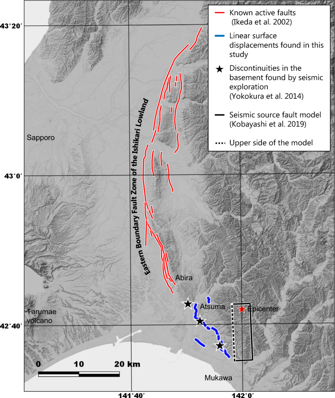
Linear surface displacements (blue lines) detected by SAR interferograms and known active faults (red lines marking the Eastern Boundary Fault Zone of the Ishikari Lowland; Ikeda et al. 2002) on shaded topography. Black stars indicate the positions of discontinuities in the basement found by seismic exploration (Yokokura et al. 2014). The red star shows the epicenter of the 2018 Hokkaido Eastern Iburi Earthquake (Earthquake Research Committee 2018). The black rectangle indicates a source fault plane (projected on the map) modeled by Kobayashi et al. (2019) and the dotted line indicates the upper side of the model
-
(2)
The east–west shortening displacement was ~ 5–10 cm, generally larger than the crustal deformation modeled by the main earthquake fault model (Kobayashi et al. 2019).
-
(3)
Vertical displacement was rather small and clear vertical displacement appeared only at the southern end of the lineament (cross section b3 in Fig. 7).
-
(4)
According to (1), (2), and (3) above, the displacement along these features can thus be described as reverse fault motion with a low dip angle.
-
(5)
The strike and displacement (east–west shortening along the reverse fault) matches the surrounding topography and tectonics, but these features have not been recognized as active faults (Earthquake Research Committee 2010; Ikeda et al. 2002).
-
(6)
These linear surface displacements exist on the SSE extension of the Eastern Boundary Fault Zone of the Ishikari Lowland (Figs. 1, 8).
-
(7)
The surface trace of the linear surface displacements is not a straight line but a somewhat complicated curve that roughly follows the terrain, situated between the eastern side of the Ishikari Lowland and the western side of the Yubari Mountains. Thus, these features have some correlation to the topography (Fig. 7).
-
(8)
Seismic exploration by Yokokura et al. (2014) recognized discontinuities in the basement just under the linear surface displacements; these may be traces of a hidden fault (black stars in Figs. 5, 6, 8).

Liquefaction in coastal areas
In the coastal town of Mukawa, in the southern part of the study area, several localized areas of hundreds of meters in diameter moved up by 50 cm (Fig. 9). Unfortunately, the image quality of Fig. 9b is poor and the resolution is lower than that of Fig. 9a because of multi-look filtering to reduce noise. The ground deformation shown in Fig. 9a, b generally has opposite values (site 2 in Fig. 9b is not clear owing to decorrelation and for site 2′ it is easy to recognize the values), making it most likely that horizontal displacement in the east–west direction was dominant and vertical displacement was small in this area.

However, the distribution of displacements was complex. At site 1 in Fig. 9, the displacement was ~ 10 cm westward, at site 2 it was ~ 50 cm eastward, and at site 3 it was ~ 5 cm eastward. In addition, the coherence of the interferograms around sites 4 and 5 was low and the form of displacement was not uniform, suggesting that relatively random displacements occurred. In an aerial photograph taken after the earthquake (GSI 2018a), traces of jetted sand were found in a baseball field close to site 1. As this location is near the coast, there is a possibility that lateral spread occurred owing to liquefaction caused by the seismic motion.
Liquefaction in fill land valleys
In a residential area within the southern part of the city of Sapporo, far from the epicenter, damage including road subsidence and tilted houses was caused by earthquake-induced liquefaction (Konagai et al. 2018). These deformation areas were detected based on the SAR interferogram (Fig. 10a) and the normalized coherence-change map (Fig. 10b). Surface displacement detected by comparisons of SAR observations before and after the earthquake mostly shows subsidence of several centimeters, but estimates from aerial photographs (GSI 2018a) suggest displacement amounts exceeding 1 m in some places where the coherence of the interferograms was greatly reduced. In Fig. 10b, the areas most affected (as determined through interpretation of aerial photographs) coincided with the area where the largest normalized coherence changes were observed.

SAR interferogram (a), normalized coherence-change map (b), and change in topography (c) in the southern part of the city of Sapporo showing liquefaction. a SAR interferogram, using image pair 4 (Table 1). Black lines indicate areas where subsidence and surface changes were estimated using Fig. 10a, b. b Normalized coherence change of SAR image pairs 2 and 4. Gray shading indicates areas where coherence before the earthquake was < 0.5. Blue arrows indicate areas experiencing significant sediment-related damage as interpreted from aerial photographs. Black lines are the same as in a. c Change in topography due to cut-and-fill activity as detected in aerial photographs. Black lines are the same as in a
By reconstructing the past topography (altitude) from aerial photographs, we obtained changes in topography due to human cut/fill operations (Fig. 10c) during a period of urban development beginning in the 1960s. The recent deformation areas coincided remarkably with the filled areas (ex-valleys), implying that earthquake-related liquefaction likely occurred in these areas (Konagai et al. 2018). These results clearly indicate that mapping topography changes due to man-made operations can be applied to urban planning and/or safety assessment in other areas.
Landslides in mountainous areas
Strong seismic motions triggered many landslides in the mountainous area surrounding the epicenter (Figs. 11, 12). The Ministry of Land, Infrastructure, Transport and Tourism (2018) estimated that the total affected area as ~ 13.4 km2, exceeding the 1891 Nobi and the 2004 Niigataken Chuetsu earthquakes, the largest to occur in inland Japan in the last 150 years. Yamagishi and Yamazaki (2018) pointed out that most landslides slid over unstable pumice and ash layers deposited by past large eruptions of the Shikotsu caldera and the Mt Eniwa-dake and Mt Tarumae volcanoes.


Landslides and InSAR coherence analysis in a mountainous area. a Landslides interpreted by aerial photographs (dark blue; GSI 2018b) on shaded relief map; location shown in Fig. 11. Pink indicates areas where the normalized phase noise deviation was small enough for the phase unwrapping in Figs. 5 and 6. Black arrows indicated the location of a large landslide that caused the collapse of many houses. b Aerial photograph from after the earthquake. Black arrows are the same as in a. c Normalized coherence change of SAR image pairs 1 and 3. Gray shading indicates masked areas where the coherence before the earthquake was < 0.2. Black arrows are the same as in a. d Normalized coherence change of SAR image pairs 2 and 4. Gray shading indicates masked areas where the coherence before the earthquake was < 0.2. Black arrows are the same as in a
For example, a large landslide at the foot of a small mountain caused the collapse of many houses (Fig. 12a, b). Although coherence-change maps clearly show high values in this area (Fig. 12c, d), in other areas they are likely over-estimated. Since the coherence-change maps have many mis-estimations in no landslide areas, it is difficult to fully understand the situation. The normalized phase deviation map (Fig. 12a) shows that, although fine changes could not be captured owing to the spatial filter, the distribution of the overall landslide area was well-extracted in Figs. 11 and 12a because of small over-estimation in contrast with the coherence-change maps. Therefore, coherence-change maps can be used to analyze detailed distributions in surface change related to such events, and normalized phase deviation maps can be used to estimate overall affected areas for rapid response or mitigation.
Discussion
Connection between linear surface displacements and the seismic fault
The depth of the main earthquake’s hypocenter (obtained from the seismic wave) was ~ 35 km (Earthquake Research Committee 2018). Furthermore, the seismic source fault model obtained from the crustal deformation showed that the depth of the fault plane’s top was ~ 16 km and it had a dip angle of 74° (Kobayashi et al. 2019). Based on the surface displacements shown in Figs. 5 and 6, the linear surface displacement features represent the movement of the reverse fault along its low dip angle. In addition, the horizontal distance from the linear surface displacements to the epicenter was ~ 10 km (Fig. 8). The known active faults on the north side of the linear surface displacements had low dip angles at 3 km depth and almost zero at 2 km depth (Earthquake Research Committee 2010; Ikeda et al. 2002; Yokokura et al. 2014).
Given these facts, if the linear surface displacements are considered to be directly connected to the hypocenter, the fault’s low dip angle at shallow depth must change to a high dip angle at around 30 km depth. Therefore, it is unlikely that the linear surface displacements directly connect with the focal seismic fault. Furthermore, since few aftershocks were observed at depths < 10 km (Earthquake Research Committee 2018), even if the linear surface displacements were structurally connected to the hypocenter, it is almost impossible that the motion of the linear surface displacements was directly linked to the fault movement at the hypocenter.
Nature of linear surface displacements
Similar linear surface displacements induced by other large earthquakes were first presented by Sangawa et al. (1985) with respect to faults on the western coast along the southern part of Suruga Bay in central Japan; these had not caused a large earthquake independently but had moved as a result of other large earthquakes. Recently, Fujiwara et al. (2016) identified more than 200 linear surface displacements associated with the 2016 Kumamoto Earthquake that shared some common features with those in this study:
-
(1)
The typical length was several kilometers or more, with linear or gentle curvilinear shapes, and displacements of a few centimeters to several tens of centimeters.
-
(2)
Many were far from the seismogenic fault, making it unlikely that they were directly connected.
-
(3)
There is no evidence that they generated strong seismic waves at the time of the main earthquake.
-
(4)
They likely moved passively and are considered results of, not the cause of, the main earthquake.
-
(5)
Given the correlation between topography and displacement, some have been recognized as active faults from their topographical features. Therefore, there is a possibility that similar movements have occurred in the past.
-
(6)
Their strike directions and displacement patterns are consistent with the surrounding stress field over a wide region.
Furthermore, Kobayashi et al. (2019) pointed out that a ΔCFF estimate suggests that the static stress change due to the 2018 Hokkaido Eastern Iburi Earthquake could have encouraged reverse slip in the area around the linear surface displacements of several dozen kilopascals. Given this context, the linear surface displacements were likely produced by secondary non-seismogenic fault motions passively generated by the 2018 Hokkaido Eastern Iburi Earthquake.
As for the independent horizontal movement in area D (Figs. 5, 6), other independent movements were found in the Mukawa area (Fig. 9). Because the latter occurred in flat coastal areas, they can be considered as lateral spread related to liquefaction. Although the movement of area D was similar to that in Mukawa, the former was situated on a slightly elevated area and seems not to have moved by lateral spreading. Togo (2000) pointed out that the surface expression of a reverse fault tends to move forward (the lower side of the fault), generating a new fault plane, and so area D may be a fault expression shaped by erosion.
Alternatively, area D could have remained in place while the surrounding area moved east (similar to lateral spreading). In this scenario, since the whole area should have shifted fairly uniformly to the east, a uniform horizontal slip must have occurred at a certain depth over a wide area of ~ 15 km N–S and ~ 5 km E–W. Fully understanding the complex movements of area D requires further study.
Use of linear surface displacements to recognize active faults
Although there is no evidence that the linear features considered in this study generated strong seismic waves at the time of the main earthquake, there is a possibility that these represent surface traces of active faults and could cause large earthquakes in the future. At present, we can provide no concrete answer to this question.
As shown in Fig. 8, the linear surface displacements appear to be geographical extensions of the known active faults. In addition, their strikes and displacements match surrounding geological features and fault-like structures were found just beneath them by a seismic reflection survey (Yokokura et al. 2014). Such circumstantial evidence sufficiently indicates that these features are most likely the traces of active faults.
Some of the linear surface displacements recognized after the 2016 Kumamoto Earthquake included those that had been identified as active faults by their topography, but the number was limited (Fujiwara et al. 2016). However, the linear surface displacements detected after the 2018 Hokkaido Eastern Iburi Earthquake had not been identified as active faults. One of the possible reasons why previous studies could not map these lineaments as ‘active faults’ is that the lineaments were not straight lines owing to the low dip angle. Even in this situation, our results support the existence of hidden faults, of which the linear surface displacements are most likely surface traces. On this basis, the detection of linear surface displacements can be used for active fault identification in the future.
However, it is also likely that those previously recognized ‘active faults’ from their topographical features did not generate seismic waves, either. Therefore, it is important to recognize the diversity of ‘active faults’ for earthquake hazard assessment.
Coherence analysis in mountainous and urban areas
Figures 10b and 12c, d show normalized coherence-change maps obtained by the same method. In Fig. 10b, fluctuations associated with liquefaction in urban areas can be clearly detected. Although Fig. 12c, d clearly shows the landslide distribution in the mountains, it is possible that these features were excessively extracted (see also Additional file 1: Fig. S4). There are two possible reasons for this: the sensitivity of the normalized coherence change could be too high, or the original coherence was too low in the mountains. In urban areas, the presence of buildings and pavements means that changes in the surface itself are relatively small, but in mountainous areas sediment moves more freely, and thus surface conditions can change more significantly. Although normalized coherence change is capable of detecting minute deformations, it does have a tendency toward saturation. Thus, in mountainous landslide-prone areas, it is possible that small displacements or changes occurring near actual landslides could be detected and classified as actual landslides.
Although the normalized coherence-change method is inaccurate in areas with low coherence, it can be corrected by masking those areas using a coherence filter for the pre-earthquake image (Watanabe et al. 2016). We used masks of 0.5 or less in the urban area (Fig. 10b) and of 0.2 in the mountainous area (Fig. 12c, d). In the latter, adopting a mask of 0.5 or less could improve the accuracy, but since the coherence was extremely low, values could not be obtained in most places using the coherence filter. Therefore, it was difficult to detect coherence changes in mountainous areas, and other methods such as multi-polarimetry (Watanabe et al. 2016), should be considered.
On the contrary, in areas masked using the normalized phase noise deviation (Figs. 11, 12a, and Additional file 1: Fig. S4b), the degradation area (large phase variation) of the SAR interferogram roughly agreed with the landslide area interpreted by the aerial photographs. Consequently, the normalized phase noise deviation can be used to roughly estimate the spatial distribution of landslide concentration areas for rapid response or mitigation.
Conclusions
We used satellite SAR interferometry to identify and interpret surface displacements associated with the 2018 Hokkaido Eastern Iburi Earthquake with the following conclusions:
-
(1)
Linear surface displacements appeared west of the epicenter. Given the distance between these features and the hypocenter and aftershocks, it is unlikely that the former are directly connected to the main earthquake fault.
-
(2)
The linear surface displacements were located along the geographic extension of known active faults (the Eastern Boundary Fault Zone of the Ishikari Lowland); structural discontinuities in the basement were found just beneath them by previous seismic exploration. They are also situated along the boundary between the lowland and the mountains. Therefore, these features are most likely the surface expression of unknown active faults, and detection of their linear surface displacements can be used for active fault identification.
-
(3)
The SAR interferograms clearly show displacement caused by liquefaction in urban fill and coastal areas.
-
(4)
Coherence-change analysis of the SAR interferograms is a useful tool for detecting surface changes caused by liquefaction as well as landslides, owing to its high sensitivity.
-
(5)
Phase noise deviation could roughly identify landslide concentration areas, producing maps useful for estimating overall affected areas for rapid response or mitigation.
Results (3), (4), and (5) show that combination of SAR interferograms, coherence-change analysis, and phase noise deviation mapping potentially allows for better mapping of local hazards in areas affected by strong quakes, and can be applied to future urban planning and/or safety assessments.
Availability of data and materials
The datasets used and/or analyzed during the current study are available from the corresponding author on reasonable request.
References
Earthquake Research Committee (2010) Evaluation of the eastern boundary fault zone of the Ishikari Lowland. https://www.jishin.go.jp/main/chousa/katsudansou_pdf/06_ishikari-teichi_2.pdf. Accessed 22 Jan 2019 (in Japanese)
Earthquake Research Committee (2018) Evaluation of the 2018 Hokkaido Eastern Iburi Earthquake. https://www.jishin.go.jp/main/chousa/18oct_iburi/index-e.htm. Accessed 22 Jan 2019
Fujiwara S, Rosen PA, Tobita M, Murakami M (1998) Crustal deformation measurements using repeat-pass JERS 1 synthetic aperture radar interferometry near the Izu Peninsula, Japan. J Geophys Res 103:2411–2426. https://doi.org/10.1029/97JB02382
Fujiwara S, Nishimura T, Murakami M, Nakagawa H, Tobita M, Rosen PA (2000) 2.5-D surface deformation of M6.1 earthquake near Mt Iwate detected by SAR interferometry. Geophys Res Lett 27:2049–2052. https://doi.org/10.1029/1999GL011291
Fujiwara S, Yarai H, Kobayashi K, Morishita Y, Nakano T, Miyahara B, Nakai H, Miura Y, Ueshiba H, Kakiage Y, Une H (2016) Small-displacement linear surface ruptures of the 2016 Kumamoto earthquake sequence detected by ALOS-2 SAR interferometry. Earth Planets Space 68:160. https://doi.org/10.1186/s40623-016-0534-x
Geospatial Information Authority of Japan (2018a) Aerial photographs of the 2018 Hokkaido Eastern Iburi Earthquake. http://www.gsi.go.jp/BOUSAI/H30-hokkaidoiburi-east-earthquake-index.html#1. Accessed 22 Jan 2019 (in Japanese)
Geospatial Information Authority of Japan (2018b) Landslide map of the 2018 Hokkaido Eastern Iburi Earthquake. http://www.gsi.go.jp/BOUSAI/H30-hokkaidoiburi-east-earthquake-index.html#10. Accessed 22 Jan 2019 (in Japanese)
Geospatial Information Authority of Japan (2018c) Overview and types of digital elevation model of fundamental geospatial data. https://fgd.gsi.go.jp/download/ref_dem.html. Accessed 22 Jan 2019 (in Japanese)
Hanssen R (2001) Radar interferometry: data interpretation and error analysis. Springer, Dordrecht. https://doi.org/10.1007/0-306-47633-9
Ikeda Y, Imaizumi T, Togo M, Hirakawa K, Miyauchi T, Sato H (eds) (2002) Atlas of quaternary thrust faults in Japan. Univ Tokyo Press, Tokyo (in Japanese)
Kobayashi T, Hayashi K, Yarai H (2019) Geodetically estimated location and geometry of fault plane involved in the 2018 Hokkaido Eastern Iburi Earthquake. Earth Planets Space. https://doi.org/10.1186/s40623-019-1042-6
Konagai K, Nishiyama S, Ohishi K, Kodama D, Nanno Y (2018) Large ground deformations caused by the 2018 Hokkaido Eastern Iburi Earthquake. JSCE J Disaster Fact Sheets FS2018-E-0003:1–8
Ministry of Land, Infrastructure, Transport and Tourism (2018) Comparison of the collapse area of the Hokkaido Eastern Iburi Earthquake and past earthquakes. http://www.mlit.go.jp/river/sabo/h30_iburitobu/181005_sediment_volume.pdf. Accessed 22 Jan 2019 (in Japanese)
Morishita Y, Hanssen R (2015) Temporal decorrelation in L-, C-, and X-band satellite radar interferometry for pasture on drained peat soils. IEEE Trans Geosci 53:1096–1104. https://doi.org/10.1109/TGRS.2014.2333814
Rosen PA, Hensley S, Zebker HA, Webb FH, Fielding EJ (1996) Surface deformation and coherence measurements of Kilauea Volcano, Hawaii, from SIR-C radar interferometry. J Geophys Res 101:23109–23125. https://doi.org/10.1029/96JE01459
Sangawa A, Katurajima S, Miyazaki J (1985) Active faults in the southern part of Suruga Bay West Coast. In: Proceedings Seismological Society of Japan C92 (in Japanese)
Togo M (2000) Geomorphological analysis on surface ruptures by reverse faulting in Japan. Kokon, Tokyo (in Japanese)
Watanabe M, Thapa RB, Ohsumi T, Fujiwara H, Yonezawa C, Tomii N, Suzuki S (2016) Detection of damaged urban areas using interferometric SAR coherence change with PALSAR-2. Earth Planets Space 68:131. https://doi.org/10.1186/s40623-016-0513-2
Yamagishi H, Yamazaki F (2018) Landslides by the 2018 Hokkaido Iburi-Tobu Earthquake on September 6. Landslides 15:2521–2524. https://doi.org/10.1007/s10346-018-1092-z
Yokokura T, Okada S, Yamagishi K (2014) Subsurface geological structure revealed by seismic reflection surveys around the southern part of the Eastern Boundary Fault Zone of the Ishikari Lowland, Hokkaido, Japan. Seamless Geoinformation of Coastal Zone “Southern Coastal Zone of the Ishikari Depression”. Geological Survey of Japan. Tsukuba (in Japanese with English abstract)
Acknowledgements
ALOS-2 data were provided by the Earthquake Working Group under a cooperative research contract with JAXA. The ALOS-2 data belong to JAXA.
Funding
This work was supported by the Geospatial Information Authority of Japan.
Author information
Authors and Affiliations
Contributions
SF mapped the local displacements and drafted the manuscript. YM, TK, and HY analyzed the interferograms. TN analyzed the aerial photographs. HU analyzed the active fault data. KH constructed the interferograms. All authors read and approved the final manuscript.
Corresponding author
Ethics declarations
Ethics approval and consent to participate
Not applicable.
Consent for publication
Not applicable.
Competing interests
The authors declare that they have no competing interests.
Additional information
Publisher's Note
Springer Nature remains neutral with regard to jurisdictional claims in published maps and institutional affiliations.
Additional file
Additional file 1.
Fig. S1. ALOS-2 SAR interferogram of image pair 3 (Table 1) on shaded relief topography. The red star shows the epicenter of the 2018 Hokkaido Eastern Iburi Earthquake (Earthquake Research Committee 2018). Fig. S2. ALOS-2 SAR interferogram of image pair 4 (Table 1) on shaded relief topography. The red star shows the epicenter of the 2018 Hokkaido Eastern Iburi Earthquake (Earthquake Research Committee 2018). Fig. S3. ALOS-2 SAR interferogram of image pair 5 (Table 1) on shaded relief topography. The red star shows the epicenter of the 2018 Hokkaido Eastern Iburi Earthquake (Earthquake Research Committee 2018). Fig. S4. Landslides and InSAR coherence analysis in a mountainous area. (a) Landslides interpreted from aerial photographs (dark blue; GSI 2018b). The blue dashed line shows the rough area of landslide concentration. (b) Pink shading indicates areas where the normalized phase noise deviation was small enough for the phase unwrapping in Figs. 5 and 6. The blue dashed line is the same as in (a). (c) Normalized coherence change of SAR image pairs 1 and 3. Gray area is the masked area where the coherence before the earthquake was smaller than 0.2. Blue dashed line is the same as in (a). (d) Normalized coherence change of SAR image pairs 2 and 4. Gray area is the same as in (c). The blue dashed line is the same as in (a).
Rights and permissions
Open Access This article is distributed under the terms of the Creative Commons Attribution 4.0 International License (http://creativecommons.org/licenses/by/4.0/), which permits unrestricted use, distribution, and reproduction in any medium, provided you give appropriate credit to the original author(s) and the source, provide a link to the Creative Commons license, and indicate if changes were made.
About this article

Cite this article
Fujiwara, S., Nakano, T., Morishita, Y. et al. Detection and interpretation of local surface deformation from the 2018 Hokkaido Eastern Iburi Earthquake using ALOS-2 SAR data. Earth Planets Space 71, 64 (2019). https://doi.org/10.1186/s40623-019-1046-2
Received:
Accepted:
Published:
DOI: https://doi.org/10.1186/s40623-019-1046-2