
Abstract
The pseudo point-source model approximates the rupture process on faults with multiple point sources for simulating strong ground motions. A simulation with this point-source model is conducted by combining a simple source spectrum following the omega-square model with a path spectrum, an empirical site amplification factor, and phase characteristics. Realistic waveforms can be synthesized using the empirical site amplification factor and phase models even though the source model is simple. The Kumamoto earthquake occurred on April 16, 2016, with M JMA 7.3. Many strong motions were recorded at stations around the source region. Some records were considered to be affected by the rupture directivity effect. This earthquake was suitable for investigating the applicability of the pseudo point-source model, the current version of which does not consider the rupture directivity effect. Three subevents (point sources) were located on the fault plane, and the parameters of the simulation were determined. The simulated results were compared with the observed records at K-NET and KiK-net stations. It was found that the synthetic Fourier spectra and velocity waveforms generally explained the characteristics of the observed records, except for underestimation in the low frequency range. Troughs in the observed Fourier spectra were also well reproduced by placing multiple subevents near the hypocenter. The underestimation is presumably due to the following two reasons. The first is that the pseudo point-source model targets subevents that generate strong ground motions and does not consider the shallow large slip. The second reason is that the current version of the pseudo point-source model does not consider the rupture directivity effect. Consequently, strong pulses were not reproduced enough at stations northeast of Subevent 3 such as KMM004, where the effect of rupture directivity was significant, while the amplitude was well reproduced at most of the other stations. This result indicates the necessity for improving the pseudo point-source model, by introducing azimuth-dependent corner frequency for example, so that it can incorporate the effect of rupture directivity.

.
Background
Strong ground motions were recorded at many stations during the Kumamoto earthquake of April 16, 2016 that occurred at 01:25 (JST), with M JMA 7.3. Some records exceeded a peak ground velocity (PGV) of 100 cm/s, and devastating damage was caused. Source modeling of the earthquake by simulating strong ground motions is important for predicting strong ground motions and understanding their generation mechanism. Researchers have conducted source process analyses of the earthquake. For example, Yagi et al. (2016) and Yamanaka (2016) estimated the source process using teleseismic records. Koketsu (2016), Asano and Iwata (2016), Kubo et al. (2016), and Nozu (2016) used strong ground motions. These analyses indicated that the rupture propagated mainly toward the northeast from the hypocenter, and the rupture extended almost as far as the western edge of Mount Aso. This kind of rupture propagation can cause the rupture directivity effect, where seismic waves are coherently superposed. In the 2016 Kumamoto earthquake, strong motions observed northeast of the epicenter could be amplified by the forward directivity effect. Strong ground motion simulations using point-source models do not seem appropriate for such earthquakes. However, the pseudo point-source model proposed by Nozu (2012a) has been successfully applied to large earthquakes such as the 2011 Tohoku earthquake (Nozu 2012a) as well as shallow crustal earthquakes (Hata and Nozu 2014), although the source model does not consider the rupture directivity effect.
In this study, a pseudo point-source model of the 2016 Kumamoto earthquake was built, and strong ground motions were simulated with the model. The target frequency range was 0.2–10 Hz, which was higher than that of the waveform inversions, so as to focus on damage caused to structures. Then, the proposed source model and the effect of rupture propagation were investigated by comparing the synthetic and observed records, in both the forward and backward regions.
Methods
In the pseudo point-source model, strong ground motions are generated from subevents that are placed on the fault plane. Each subevent is approximated with a point source, and may correspond to strong-motion generation areas (SMGAs) (e.g., Kamae and Irikura 1998) or strong-motion pulse generation areas (SPGAs) (Nozu 2012b) in the characterized source models. However, the pseudo point-source model does not consider the spatiotemporal distribution of the slip within the subevent explicitly for the purpose of simplification. Instead, a subevent is modeled by a source spectrum that follows the omega-square model (Aki and Richards 2002). The current version of the pseudo point-source model assumes the same corner frequency for any azimuth or take-off angle. In this respect, the pseudo point-source model is different from SMGA or SPGA models, in which the rupture propagation within a finite subevent is explicitly modeled to consider the directivity effect. Directivity is one possible source of discrepancy from the observed records when the pseudo point-source model is applied to large earthquakes.
In the application of the pseudo point-source model, path spectrum, site amplification spectrum, and phase spectrum must be evaluated along with the source spectrum to obtain synthetic waveforms. The synthetic waveforms are calculated using the inverse Fourier transform of the spectrum A(f) at a target station. A(f) is calculated as
where S(f) is the source spectrum; P(f) the path spectrum; G(f) the site amplification spectrum that represents the amplification in the sedimentary layer; and O(f)/|O(f)|p the phase spectrum, where f is the frequency.
S(f) is given by Boore (1983) as
where R θϕ is the radiation coefficient; PRTITN the coefficient to divide the seismic energy into two horizontal components; FS the amplification due to the free surface (=2.0); M the seismic moment; and f c the corner frequency. Furthermore, ρ and Vs are the density and the shear wave velocity in the source region, respectively. In the pseudo point-source model, the finiteness of the subevent is implicitly incorporated by f c , which is inversely proportional to the square root of the area of the subevent.
P(f) is given by Boore (1983) as
where r is the distance from the source to the site and Q is the quality factor.
For G(f)s, we basically use the empirical model evaluated by Nozu et al. (2006) with the generalized inversion technique, using many weak motions for K-NET and KiK-net stations (Aoi et al. 2004; Okada et al. 2004). However, as described later, G(f) values for several stations were estimated in this study.
The phase spectrum is also evaluated with an empirical model. O(f) is the Fourier transform of a small earthquake record observed at a target station, and |O(f)|p is the absolute value of O(f) to which a Parzen window of 0.05 Hz bandwidth is applied. Here the absolute value is calculated first, and then the Parzen window is applied. O(f)/|O(f)|p is thus a complex spectrum that has small ripples and whose absolute value is almost one. These small ripples are necessary for generating causal waveforms (Nozu and Sugano 2008). If there is more than one subevent, the contribution from each subevent is superposed with the appropriate delay time. In summary, the source and path spectra are evaluated by simple formulas in the model, whereas the site amplification and phase spectra are evaluated empirically. Because of the simplicity of the source model, only six parameters are necessary for each subevent: longitude, latitude, depth, seismic moment, corner frequency, and rupture time. We need to determine the number of subevents and the parameters for each subevent.
Parameters
Twelve K-NET and KiK-net stations were used in the source modeling, as shown in Fig. 1. We adopt the hypocentral parameters determined by JMA (2016) and assume one fault plane with strike of 232° and dip of 84° according to Nozu (2016). The subevents were placed on this plane. Density and S-wave velocity in the source region of 2400 kg/m3 and 3.55 km/s were used, respectively, from F-net (Fukuyama et al. 1998). Q was assumed to be 104f 0.63 from Kato (2001).

Locations of the epicenter, target stations, and proposed subevents
As mentioned before, G(f) was basically obtained from Nozu et al. (2006), but values of G(f) for KMM006 and KMMH16 were newly evaluated in this study. This is because the location of KMM006 was moved in 2015, and G(f) at KMMH16 was evaluated based on only two records in Nozu et al. (2006). The modified G(f)s for KMM006 and KMMH16 were evaluated using spectral ratios of weak motions. Considering the importance of KMMH16, which is very close to the epicenter of the mainshock, G(f) for the borehole sensor at KMMH16 was newly evaluated. G(f)s were evaluated only for surface sensors in Nozu et al. (2006). Reevaluation was conducted as follows:
-
1.
Reevaluate the G(f) at the surface of KMMH16 by multiplying the observed Fourier spectral ratio (KMMH16 surface/previous KMM006) and the G(f) at the previous KMM006 by Nozu et al. (2006). The observed Fourier spectral ratio was evaluated using five weak motions before the relocation of KMM006 (Table 1).
Table 1 Earthquakes used to reevaluate the G(f) at KMMH16 (surface) -
2.
Evaluate G(f) at the present KMM006 by multiplying the observed Fourier spectral ratio (present KMM006/KMMH16 surface) and the reevaluated G(f) at the surface of KMMH16. The observed Fourier spectral ratio was evaluated using eight weak motions after the relocation of KMM006 (Table 2).
Table 2 Earthquakes used to reevaluate the G(f) at KMM006 after relocation -
3.
Evaluate G(f) at the borehole of KMMH16 by multiplying the observed Fourier spectral ratio (KMMH16 borehole/KMMH16 surface) by the reevaluated G(f) at the surface of KMMH16. The observed Fourier spectral ratio was evaluated using the same eight weak motions as in step 2 of the procedure (above).
-
4.
Compare the G(f)s before and after modification. These three newly evaluated G(f)s are shown in Fig. 2, which shows that G(f) for the surface of KMMH16 increased slightly, although not significantly.
Fig. 2 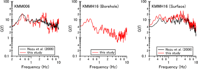
Reevaluated site amplification factor G(f) at KMM006 and KMMH16 (surface) as well as newly evaluated G(f) at KMMH16 (borehole)

In addition to the site amplification factors, we needed to select an earthquake for the phase characteristics O(f). The earthquake was selected by comparing the waveforms of the target earthquake with the waveforms calculated from the Fourier amplitude of the target earthquake and the Fourier phase of a small earthquake. We tested 19 earthquakes for O(f) and ultimately selected the earthquake of April 16, 2016, that occurred at 04:51 (JST) with M JMA 4.3. This earthquake occurred very close to the mainshock. Several examples of comparisons of the velocity waveforms (0.2–2 Hz) are shown in Fig. 3. Figure 3 shows that the main features of the mainshock ground motions are basically explained by the synthetic waveforms. Figure 3 also shows the variance reduction for each component. An average variance reduction of 0.40 for eight components was achieved for this small earthquake. At some stations, the nonlinear soil response was considered in the simulation of strong ground motions, as will be explained later.

Comparison of phase characteristics between the mainshock and a small earthquake. A band-pass filter (0.2–2 Hz) is applied. The phase characteristics of the red lines are from the earthquake that occurred on April 16, 2016, at 04:51 (JST) with MJMA4.3. Variance reduction (VR) is calculated using a section of 10 s starting from the arrival of S-wave
Figure 4 shows the comparison of the observed acceleration Fourier spectra and the G(f)s at 12 stations. There are some troughs in the observed Fourier spectra that are not seen in the site amplification spectra. For example, clear troughs are seen at KMMH16 on both the borehole and surface records in Fig. 4. These troughs were considered to be generated by interference of seismic waves from different subevents. Based on such examination, two subevents, Subevent 1 and Subevent 2, were placed on the fault plane near the hypocenter (Fig. 1). In addition, Subevent 3 was placed on the northeastern part of the fault plane, where a large slip and slip velocity were indicated by waveform inversion analyses (Fig. 1). The parameters of the subevents were determined as shown in Table 3.

Observed Fourier spectrum and site amplification spectrum G(f). Black line observed Fourier spectrum; red line site amplification spectrum G(f); solid line on the surface; and dotted line in the borehole. Observed records (black lines) are smoothed by a Parzen window of 0.05 Hz bandwidth. Peak frequencies are indicated by arrows
Subevents 1 and 2 are mainly responsible for the strong motions at stations, except for those located northeast of the source region. Subevent 3 was placed to reproduce strong motions at the stations northeast of the source region listed in Table 3, as shown in the next section. The location of Subevent 1 was determined considering the arrival time of strong motions at the borehole sensors of KMMH14 and KMMH16 and the surface sensors of KMM006 and KMMH16 (Table 4; Fig. 5). Although uncertainty of a few kilometers may exist because of insufficient information regarding the detailed velocity structure, the depth of 18 km is consistent with the results of source process analyses (Koketsu 2016; Asano and Iwata 2016; Nozu 2016) that suggest that the rupture propagated deep near the hypocenter. The relative locations of Subevents 1 and 2 (distance of 2.3 km and delay time of 1.1 s) are determined to reproduce the characteristic troughs in the Fourier spectra at KMMH16.

Arrival time of the strong motions of the mainshock. Time 0 s in the figure is 1:25:00 (JST)
The seismic moment and corner frequency of Subevents 1 and 2 were determined such that the average Fourier spectrum error at the stations (shown in Fig. 1) is minimized under the constraint that the seismic moment of Subevent 1 is smaller than that of Subevent 2. Here, the Fourier spectrum error was defined as
where FS obs is the observed Fourier spectrum and FS syn the synthetic Fourier spectrum. The restriction on the seismic moment was imposed because the amplitude of the synthetic waveforms was not consistent with the observed amplitude if the seismic moment of Subevent 1 was greater than that of Subevent 2. Figure 6 shows the synthetic velocity waveforms calculated using the parameters that minimize the Fourier spectrum error without restricting the seismic moment. The parameters were determined as follows: The seismic moments of Subevents 1 and 2 are 7.0 × 10¹⁷ and 3.0 × 10¹⁷ Nm, respectively, and the corner frequencies of Subevents 1 and 2 are 0.6 and 0.5 Hz, respectively. As a result, a strong pulse was not reproduced at all in this case, as shown in Fig. 6; the seismic moment of Subevent 2 has to be greater than that of Subevent 1 to better reproduce the amplitude of the observed waveforms. In the search for these parameters, Subevent 3 was neglected because it was found unnecessary for minimizing the Fourier spectrum error. Subevent 3 corresponds to the area with large slip, as indicated by waveform inversion analyses (Koketsu 2016; Asano and Iwata 2016; Nozu 2016; Kubo et al. 2016). The region was considered to have caused forward and backward directivity to the stations northeast and southwest of Subevent 3, respectively. In other words, Subevent 3 generated stronger seismic waves to the northeast. The current version of the pseudo point-source model, on the contrary, does not consider rupture propagation and assumes the same amplitude, independent of the azimuth. As a result, Subevent 3 cannot contribute to reducing the Fourier spectrum error. Instead, the seismic moment and corner frequency of Subevent 3 were determined by a trial-and-error approach so that the observed amplitudes could be reproduced at KMMH06 where the contribution of Subevent 3 was significant. The contribution of Subevent 3 was considered only for the stations listed in Table 3. For other stations, Subevent 3 was not used in the simulation.

Difference between observed and synthetic velocity waveforms. Black line observed waveform, red line synthetic waveform. The parameters of the subevents were determined such that the averaged Fourier spectrum error for all the target stations is minimized without any constraint
As mentioned earlier, the nonlinear soil response was considered in the simulation at some stations using the simple scheme by Nozu and Sugano (2008). In general, if the shear strain in the ground is increased during strong motions, the shear modulus drops, and as a result, the shear wave velocity decreases. With a decrease in shear wave velocity, the travel time of seismic waves in the ground increases, leading to lower natural frequency in the site amplification spectrum. Thus, the effect of soil nonlinearity can be confirmed by comparing the peak frequencies of the observed Fourier spectra and the G(f)s, as shown in Fig. 4, as long as the peak frequencies are evident, because the G(f)s are evaluated using weak motion records that are not affected by soil nonlinearity. The ratio of the peak frequencies (ν1) thus indicates the ratio of the average shear wave velocity above the seismic bedrock for the linear and the nonlinear cases. Then, ν1 can be expressed as
where V Snonlinear and V Slinear are the average shear wave velocity for nonlinear and linear cases, respectively. In this study, the value ν1 was used to consider soil nonlinearity following the simple scheme of Nozu and Sugano (2008), in which the waveforms are stretched by a factor of 1/ν1 starting from the initial S-wave. An increase in the damping coefficient, which causes faster attenuation of coda waves, was also considered by Nozu and Sugano (2008); however, it was not considered in the present study for the sake of simplicity.
In general, the degree of soil nonlinearity depends on both material properties of the ground between the surface and the seismic bedrock and the amplitude of the strong ground motions. It would be convenient if we could predict the value of ν1 based on such information, especially for prediction problems. In this study, however, ν1 was determined based on the peak frequency ratio of the observed Fourier spectrum and G(f), because the ratio conveys information regarding the actual degree of soil nonlinearity during the target earthquake. This method can only be applied to those stations where G(f)s have a clear peak. Table 5 shows the list of such stations, for which the shifts of peak frequencies are indicated by arrows in Fig. 4. Although large PGVs that could cause soil nonlinearity were observed at some stations, soil nonlinearity was not considered at those stations because the peak frequencies were not clear at these stations. Evaluating soil nonlinearity at such stations is one of the future tasks.
Results and discussion
First, the synthetic Fourier spectra without considering soil nonlinearity are shown in Fig. 7 for the seven stations in Table 5 at which soil nonlinearity was considered. As shown in Fig. 7, the peak frequencies between synthetic and observed spectra did not match. In Fig. 8, the synthetic and observed Fourier spectra, including soil nonlinearity, are shown for all the target stations. The characteristics of the observed spectra were generally reproduced, and by incorporating the nonlinearity, the Fourier spectra were improved in terms of peak frequency.

Synthetic and observed Fourier spectra. Soil nonlinearity was not considered in the synthetic spectra

Synthetic and observed Fourier spectra. Soil nonlinearity was considered in the synthetic spectra. ν1 = 1.0 means that nonlinearity was not considered
On the other hand, discrepancies can be found between the synthetic and observed Fourier spectra that can be attributed to the simplicity of the pseudo point-source model. One of them is the underestimation of components lower than 0.5 Hz for almost all the stations. One possible cause of the underestimation is the shallow large slip that causes fling steps. For the 2016 Kumamoto earthquake, source process analyses using teleseismic records (Yagi et al. 2016; Yamanaka 2016) indicate that a large slip occurred near the surface, which may have contributed to the low-frequency components of the observed records. As mentioned previously, only the subevents that generate strong ground motions are modeled; therefore, shallow large slips, or fling steps, were not covered in the pseudo point-source model. Revealing the effect of shallow slip on strong ground motions is one of the important issues to be addressed. At KMMH14, located southwest of the epicenter, the synthetic Fourier spectrum overestimated the observation between 0.5 and 3 Hz. This result may indicate that the actual rupture proceeded northeast and that the backward directivity effect might appear in the observed Fourier spectrum at KMMH14.
Synthetic and observed velocity time histories (0.2–2 Hz) are shown in Fig. 9. Figure 9 shows that Subevents 1 and 2 are sufficient to reproduce strong ground motions at KMMH16 including large-amplitude pulses, although the amplitudes are somewhat underestimated. The NS component of KMMH03 is largely underestimated. This component was also underestimated by other studies, including Irikura et al. (2016), in which the empirical Green’s function method is used. The generation mechanism of the large NS component at this station is one of the important problems to be studied in the future.

Synthetic and observed velocity waveforms (0.2–2 Hz). Black line observed waveforms, red line synthetic waveforms for the final model. Subevent 3 was considered only for limited stations (see Table 3)
In Fig. 9, the rupture directivity effect of Subevent 3 can also be confirmed. Although the seismic moment and corner frequency of Subevent 3 were determined so that the observed amplitudes could be reproduced at KMMH06, the same parameters significantly underestimate the amplitudes at KMM004, as shown in Fig. 9. This is presumably due to the fact that KMM004 is located northeast of Subevent 3 where the rupture directivity effect is maximized. The need for Subevent 3 can be confirmed in Fig. 10, which shows that the synthetic velocity waveforms at the stations northeast of Subevent 3 lack some part of the waveforms if Subevent 3 is not considered. Discrepancy can also be induced in the backward side. The latter part of the waveforms was overestimated if the effects of Subevent 3 were considered at stations in the backward site, as shown in Fig. 11. These results indicate the necessity for improving the pseudo point-source model so that it can incorporate the effect of rupture directivity by, for example, introducing azimuth-dependent corner frequency. Finally, the observed and synthetic acceleration time histories are shown in Fig. 12.

Synthetic and observed velocity waveforms (0.2–2 Hz) at stations northeast of Subevent 3. Black line observed waveform, red line synthetic waveform. Synthetic waveforms were calculated without Subevent 3

Synthetic and observed velocity waveforms at stations southwest of Subevent 3. Black line observed waveforms, red line synthetic waveforms. Synthetic waveforms were calculated using Subevents 1, 2, and 3

Observed and synthetic acceleration waveforms. Black line observed acceleration waveform, red line synthetic acceleration waveform
Conclusions
We developed a pseudo point-source model for the 2016 Kumamoto earthquake of April 16 with M JMA 7.3 for the purpose of simulating strong ground motions in the frequency range of 0.2–10 Hz. Three subevents were placed on the fault plane considering the characteristics of the observed records. The synthesized Fourier spectra and velocity waveforms generally explained the observed records, such as troughs in the Fourier spectra and strong pulses. However, underestimation in the low frequency range was found. The underestimation is presumably due to the following two reasons. The first is that the target of the pseudo point-source model is only the subevents that generate strong ground motions, and it does not consider the shallow large slip. The second reason is that the current version of the pseudo point-source model does not consider the rupture directivity effect. Consequently, strong pulses were not reproduced enough at stations northeast of Subevent 3, such as KMM004, where the effect of rupture directivity was significant. This result indicates the necessity for improving the pseudo point-source model so that it can incorporate the effect of rupture directivity by, for example, introducing azimuth-dependent corner frequency.
Abbreviations
- JST:
-
Japanese standard time
- JMA:
-
Japan Meteorological Agency
- PGV:
-
Peak ground velocity
- NIED:
-
National Research Institute for Earth Science and Disaster Resilience
- SMGA:
-
Strong-motion generation area
- SPGA:
-
Strong-motion pulse generation area
References
Aki K, Richards PG (2002) Quantitative seismology, 2nd edn, University Science Books
Aoi S, Kunugi T, Fujiwara H (2004) Strong-motion seismograph network operated by NIED: K-NET and KiK-net. J Jpn Assoc Earthq Eng 4:65–74
Asano K, Iwata T (2016) Source rupture processes of the foreshock and mainshock in the 2016 Kumamoto earthquake sequence estimated from the kinematic waveform inversion of strong motion data. Earth Planets Space 68:147. doi:10.1186/s40623-016-0519-9
Boore DM (1983) Stochastic simulation of high-frequency ground motions based on seismological models of the radiated spectra. Bull Seism Soc Am 73:1865–1894
Fukuyama E, Ishida M, Dreger DS, Kawai H (1998) Automated seismic moment tensor determination by using on-line broadband seismic waveforms. Zisin 51:149–156 (in Japanese with English abstract)
Hata Y, Nozu A (2014) Pseudo point-source models for shallow crustal earthquakes in Japan. Paper presented at the second European conference on earthquake engineering and seismology, Istanbul, 25–29 August 2014
Irikura K, Miyakoshi K, Kurahashi S (2016) Methodology of simulating ground motions from crustal earthquakes and mega-thrust subduction earthquakes: application to the 2016 Kumamoto earthquake (crustal) and the 2011 Tohoku earthquake (mega-thrust). In: 5th IASPEI/IAEE international symposium: effects of surface geology on seismic motion, Taipei, 15–17 August 2016
Japan Meteorological Agency (2016) Webpage of the hypocenter list on April 16, 2016. http://www.data.jma.go.jp/svd/eqev/data/daily_map/20160416.html. Accessed 18 Oct 2016 (in Japanese)
Kamae K, Irikura K (1998) Source model of the 1995 Hyogo-ken Nanbu Earthquake and simulation of near-source ground motion. Bull Seism Soc Am 88:400–412
Kato K (2001) Evaluation of source, path, and site amplification factors from the K-NET strong motion records of the 1997 Kagoshima-Ken-Hokuseibu earthquakes. J Struct Constr Eng 543:61–68 (in Japanese with English abstract)
Koketsu K (2016) http://taro.eri.u-tokyo.ac.jp/saigai/2016kumamoto/index.html#C. Accessed July 31 2016 (in Japanese)
Kubo H, Suzuki W, Aoi S, Sekiguchi H (2016) Source rupture processes of the 2016 Kumamoto, Japan, earthquakes estimated from strong-motion waveforms. Earth Planets Space 68:161. doi:10.1186/s40623-016-0536-8
Nozu A (2012a) A simplified source model to explain strong ground motions from a huge subduction earthquake -simulation of strong ground motions for the 2011 off the Pacific Coast of Tohoku Earthquake with a pseudo point-source model. Zisin 65:45–67. doi:10.4294/zisin.65.45 (in Japanese with English abstract)
Nozu A (2012b) A super asperity model for the 2011 Off the Pacific Coast of Tohoku Earthquake. J Jpn Assoc Earthq Eng 12:221–240. doi:10.5610/jaee.12.2_21 (in Japanese with English abstract)
Nozu A (2016) http://www.pari.go.jp/bsh/jbn-kzo/jbn-bsi/taisin/research_jpn/research_jpn_2016/jr_46.html. Accessed 31 July 2016 (in Japanese)
Nozu A, Sugano T (2008) Simulation of strong ground motions based on site-specific amplification and phase characteristics–accounting for causality and multiple nonlinear effects. Technical Note of the Port and Airport Research Institute 1173. (in Japanese with English abstract)
Nozu A, Nagao T, Yamada M (2006) Simulation of strong ground motions based on site-specific amplification and phase characteristics. In: Proceedings of the third international symposium on the effects of surface geology on seismic motions, Grenoble
Okada Y, Kasahara K, Hori S, Obara K, Sekiguchi S, Fujiwara H, Yamamoto A (2004) Recent progress of seismic observation networks in Japan-Hi-net, F-net. K-net and KiK-net. Earth Planets Space 56(8):xv–xxviii. doi:10.1186/BF03353076
Yagi Y, Okuwaki R, Enescu B, Kasahara A, Miyakawa A, Otsubo M (2016) Rupture process of the 2016 Kumamoto earthquake in relation to the thermal structure around Aso volcano. Earth Planets Space 68:118. doi:10.1186/s40623-016-0492-3
Yamanaka Y (2016) http://www.seis.nagoya-u.ac.jp/sanchu/Seismo_Note/2016/NGY60.html. Accessed 31 July 2016 (in Japanese)
Authors’ contributions
YN conducted the source modeling and strong ground motion simulation. YN and AN investigated and interpreted the simulation results. Both authors read and approved the final manuscript.
Acknowledgements
We used the waveform data from K-NET and KiK-net operated by the NIED and information about the source from JMA and F-net. We would like to thank Dr. Haruo Horikawa and anonymous reviewers for their valuable comments.
Competing interests
The authors declare that they have no competing interests.
Author information
Authors and Affiliations
Corresponding author
Rights and permissions
Open Access This article is distributed under the terms of the Creative Commons Attribution 4.0 International License (http://creativecommons.org/licenses/by/4.0/), which permits unrestricted use, distribution, and reproduction in any medium, provided you give appropriate credit to the original author(s) and the source, provide a link to the Creative Commons license, and indicate if changes were made.
About this article

Cite this article
Nagasaka, Y., Nozu, A. Strong ground motion simulation of the 2016 Kumamoto earthquake of April 16 using multiple point sources. Earth Planets Space 69, 25 (2017). https://doi.org/10.1186/s40623-017-0612-8
Received:
Accepted:
Published:
DOI: https://doi.org/10.1186/s40623-017-0612-8