
Abstract
This study reports novel hybrid computational methods for the solutions of nonlinear singular Lane–Emden type differential equation arising in astrophysics models by exploiting the strength of unsupervised neural network models and stochastic optimization techniques. In the scheme the neural network, sub-part of large field called soft computing, is exploited for modelling of the equation in an unsupervised manner. The proposed approximated solutions of higher order ordinary differential equation are calculated with the weights of neural networks trained with genetic algorithm, and pattern search hybrid with sequential quadratic programming for rapid local convergence. The results of proposed solvers for solving the nonlinear singular systems are in good agreements with the standard solutions. Accuracy and convergence the design schemes are demonstrated by the results of statistical performance measures based on the sufficient large number of independent runs.
Background
Introduction
Mathematical models based on Lane–Emden type equations (LEEs) have been studied in diverse fields of applied sciences, particularly, in the domain of astrophysics. Singular second order nonlinear initial value problem (IVP) of LEEs describes various real life phenomena. Generally, the most of the problems arising in astrophysics are modelled by second order nonlinear ordinary differential equations (ODEs) (Lane 1870; Emden 1907; Fowler 1914, 1931). The general form of LFE is represented mathematically as:
for \(\alpha ,x \ge 0,\) having initial conditions as:
here a is constant and f(x, y) is a nonlinear function. LEE has a singularity at the origin, i.e., x = 0, for the above conditions. By taking \(\alpha = 2\), \(f(x,y) = y^{n}\), \(g(x) = 0\) and \(a = 1\) in the above equations, we get
with initial conditions as:
where n ≥ 0 is constant. The LEEs arise in the study of the theory of stellar structure, isothermal gas spheres, thermal behavior of a spherical cloud of gas and thermionic current models (Davis 1962; Chandrasekhar 1967; Datta 1996). Reliable and accurate solution of ODEs, with singularity behavior in various linear and nonlinear IVPs of astrophysics is a new challenge for researchers now a day.
In astrophysics, a fluid obeys a polytropic equation of state under the assumption, and then with suitable transformation laws Eq. (1) is equivalent to equation of static equilibrium. Further in case of the gravitational potential of a self-gravitating fluids the LEE is also called Poisson’s equation. Physically, hydrostatic equilibrium provides a connection between the gradient of the potential, the pressure and the density. Numerical simulation is presented in (Shukla et al. 2015) for two dimensional Sine–Gordon equation.
Analytically, it is difficult to solve these equations, so various techniques like Adomian decomposition method (ADM), differential transformation method (DTM) and perturbation temple technique based on series solutions have been used (Wazwaz 2001, 2005, 2006; Mellin et al. 1994). Ramos (2005) solved singular IVPs of ODEs using linearization procedures. Liao (2003) presented ADM for solving LEEs (Chowdhury and Hashim 2007a). Chowdhury and Hashim (2007b) employed Homotopy-perturbation method (HPM) to get the solution for singular IVPs of LEEs. Dehghan and Shakeri (2008) provides the solution of ODEs models arising in the astrophysics field using the variational iteration procedure. Further, the solution of Emden–Fowler equation (EFE) is also reported by incorporating the method of Lie and Painleve analysis by Govinder and Leach (2007). Kusano provide solutions for nonlinear ODEs based on EFEs (Kusano and Manojlovic 2011). Muatjetjeja and Khalique (2001) given the exact solution for the generalized LEEs of two kinds. Modified Homotopy analysis method (HAM) is used by Singh et al. (2009) and Mellin et al. (1994) to get the numerical solution of LEEs. Demir and Sungu (2009) gives the numerical solutions of nonlinear singular IVP of EFEs using DTM. Shukla et al. (2015) provides the studies using the cubic B-spline differential quadrature method. Moreover, neural networks applications in astronomy, Astrophysics and Space Science can be seen in Bora et al. (2008, 2009), Bazarghan and Gupta (2008), Singh et al. (1998, 2006), Gupta et al. (2004), Gulati et al. (994).
Recently, a lot of effects has been made by the researcher in the field of artificial neural networks (ANNs) to investigate the solution of the IVPs and boundary value problems (BVP) (Ahmad and Bilal 2014; Rudd and Ferrari 2015; Raja 2014a; Raja et al. 2015b). Well-established strength of neural networks as a universal function approximation optimized with local and global search methodologies has been exploited to solve the linear and nonlinear differential equations such as problems arising in nanotechnology (Raja et al. 2016b, e), fluid dynamics problems based on thin film flow (Raja et al. 2015a, 2016d), electromagnetic theory (Khan et al. 2015), fuel ignition model of combustion theory (Raja 2014b), plasma physics problems based on nonlinear Troesch’s system (Raja 2014c), electrical conducting solids (Raja et al. 2016c), magnetohydrodynamic problems (Raja and Samar 2014e) Jaffery-Hamel flow in the presence of high magnetic fields (Raja et al. 2015c), nonlinear Pantograph systems (Ahmad and Mukhtar 2015; Raja 2014d; Raja et al. 2016a) and many others. These are motivating factors for authors to develop a new ANNs based solution of differential equations, which has numerous advantages over its counterpart traditional deterministic numerical solvers. First of all, ANN methodologies provide the continuous solution for the entire domain of integration, generalized method which can be applied for the solution of other similar linear and nonlinear singular IVPs and BVPs. Aim of the present research is to develop the accurate, alternate, robust and reliable stochastic numerical solvers to solve the Lane-Enden equation arising in astrophysics models.
Organization of the paper is as follows: “Methods” section gives the proposed mathematical modelling of the system. In “Learning methodologies” section, learning methodologies are presented. Numerical experimentation based on three problems and cases is presented in “Results and discussion” section. In “Comparison through statistics” section comparative studies and statistical analysis are presented. In last section conclusions is drawn with future research directions.
Methods
Mathematical modelling
In this section, differential equation neural networks mathematical modelling of LEEs has been given. Arbitrary combine feed-forward ANNs are used to model the equation, while. Log-sigmoid based transfer function is used in the hidden layer of the networks. Following continuous mapping representing the solution y(x) and its respectively derivations is used to solve LEFs (Raja et al. 2016e; Raja 2014c).
where the ‘hat’ on the top of the symbol y(x) denotes their estimated values while δ i , β i , and ω i are bounded real-valued representing the weights of the ANN models for m the number of neurons and f is the activation function, which is equal to:
for the hidden layers of the networks.
Using log-sigmoid, ANNs based approximation of the solution and few of its derivatives can be written as:
where \(\hat{y}_{LS}^{\left( 1 \right)} \left( {\text{x}} \right)\) and \(\hat{y}_{LS}^{\left( 2 \right)} \left( {\text{x}} \right)\) represent the first and second order derivative with respect to x.
In Eq. (1), the generic form of nonlinear singular Lane–Emden equation is given. While in Eqs. (3–5) continuous mapping of neural networks models for approximate solution \(\hat{y}\left( x \right)\) and its derivatives are presented in term of single input, hidden and output layers. Additionally, in the hidden layers log-sigmoid activation function and its derivatives are used for y(t) and its derivatives, respectively.
Fitness function formulation
The objective function or fitness function is formulated by defining an unsupervised manner of differential equation networks (DEN) of given equation and its associated boundary conditions. It is defined as, where the mean square error term \(\in_{1}\) is associated with Eq. (1) is given as (Raja 2014c, d):
where \(\hat{y}_{k} = \hat{y}\left( {x_{k} } \right), N = \frac{1}{h} ,x_{k} = kh(k = 0,1,2, \ldots ,N).\)
The interval is divided into number of steps with step size and mean square error for Eq. (2) can be defined as follows:
By combining Eqs. (6) and (7), we obtain the fitness function
The ANNs architecture for nonlinear singular LEEs is presented in Fig. 1.

Design of neural network architecture for nonlinear singular Lane–Emden type equation
Learning methodologies
Pattern search (PS) optimization technique belongs to a class of direct search methods, i.e., derivative free techniques, which are suitable to solve effectively the variety of constrained and unconstrained optimization problems. Hooke et al., are the first to introduce the name of PS technique (Hooke and Jeeves 1996), while the convergence of the algorithm was first proven by Yu (1979). In standard operation of PS technique, a sequence of points, which are adapted to desire solution, is calculated. In each cycle, the scheme finds a set of points, i.e., meshes, around the desired solution of the previous cycle (Dolan et al. 2003). The mesh is formulated by including the current point multiplied by a set of vectors named as a pattern (Lewis et al. 1999). PS technique is very helpful to get the solution of optimization problem such as minimization subjected to bound constrained, linearly constrained and augmented convergent Lagrangian algorithm (Lewis et al. 2000).
Genetic algorithms (GAs) belong to a class of bio-inspired heuristics develop on the basis of mathematical model of genetic processes (Man et al. 1996). GAs works through its reproduction operators based on selection operation, crossover techniques and mutation mechanism to find appropriate solution of the problem by manipulating candidate solutions from entire search space (Cantu-Paz 2000). The candidate solutions are generally given as strings which is known as chromosomes. The entries of chromosome are represented by genes and the values of these genes represents the design variables of the optimization problem. A set of chromosome in GAs is called a population which used thoroughly in the search process. A population of few chromosomes may suffer a premature convergence where as large population required extensive computing efforts. Further details, applications and recent trends can be seen in (Hercock 2003; Zhang et al. 2014; Xu et al. 2013).
Sequential quadratic programming (SQP) belong to a class of nonlinear programming techniques. Supremacy of SQP method is well known on the basis of its efficiency and accuracy over a large number of benchmark constrained and unconstrained optimization problems. The detailed overview and necessary mathematical background are given by Nocedal and Wright (1999). The SQP technique has been implemented in numerous applications and a few recently reported articles can be seen in Sivasubramani et al. (2011), Aleem and Eldeen (2012).
In simulation studies, we have used MATLAB optimization toolbox for running of SQP, PS, and GAs as well as hybrid approaches based on PS-SQP and GA-SQP to get the suitable parameters of ANN models. The workflow diagram of the proposed methodology base on GA-SQP to get the appropriate design parameters is shown in Fig. 2 while the procedure of GA-SQP to find the optimized weight vector of ANN is given below:

Flow chart of genetic algorithm
-
Step 1: Initialization: create an initial population with bounded real numbers with each row vector represents chromosomes or individuals. Each chromosome has number of genes equal to a number of design parameters in ANN models. The parameter settings GAs are given in Table 1.
Table 1 Parameters setting for SQP, PS and GA respectively -
Step 2: Fitness evaluations: Determined the value of the fitness row vector of the population using the Eq. (7).
-
Step 3: Stoppage: Terminate GAs on the basis of following criteria.
-
The predefined fitness value \(\in\) is achieved by the algorithm, i.e., \(\in < 10^{ - 15} .\)
-
Total number of generations/iterations are executed.
-
Any of the termination conditions given in Table 1 for GAs are achieved.
If any of the stopping criteria is satisfied, then go to step 6 otherwise continue
-
Step 4: Ranking: Rank each chromosome on the basis minimum fitness \(\in\) values. The chromosome ranked high has small values of the fitness and vice versa.
-
Step 5: Reproduction: Update population for each cycle using reproduction operators based on crossover, mutation selection and elitism operations. Necessary settings of these fundamental operators are given in Table 1.
Go to step 2 with newly created population
-
Step 6: Refinement: The Local search algorithm based on SQP is used for refinement of design parameters of ANN model. The values of global best chromosome of GA are given to SQP technique as an initial start weight. In order to execute the SQP algorithm, we incorporated MATLAB build in function ‘fmincon’ with algorithm SQP. Necessary parameter settings for SQP algorithm is given in Table 1.
-
Step 7: Data Generation and analysis: Store the global best individual of GA and GA-SQP algorithm for the present run. Repeat the steps 2–6 for multiple independent runs to generate a large data set so that reliable and effective statistical analysis can be performed.
Results and discussion
The results of simulation studies are presented here to solve LEEs by the proposed ANN solver. Proposed results are compared with reported analytical as well as numerical methods.
Problem I: (Case I: n = 0)
For n = 0, the Eq. (1) becomes linear ordinary differential equation, can be written as:
and its associated conditions are
The system given in Eqs. (8–9) is solved by taking 10 neuron in ANN model and resultant 30 unknown weights \(\delta_{i} ,\beta_{i}\), and \({\kern 1pt} \omega_{i}\) for I = 1, 2,…, 10. The fitness function is developed for this case by taking step size h = 0.1 and hence 11 numbers of grid points in the interval (0, 1) as:
We have to find the weights for each model such that \(\in \,\to 0.\) The optimization of these weights is carried out using global and local approach of algorithm with parameter setting shown in Table 1. Training of weights is carried out by SQP, PS, GA, and also with a hybrid approach of PS-SQP and GA-SQP algorithms. Parameter setting given in Table 1 will be used for these algorithms. These algorithms are run and weights are trained through the function of algorithms; one specific set of weights learned by SQP, PS, GA, PS-SQP, GA-SQP algorithms yield fitness values of 1.90E−09, 4.97E−07, 6.45E−07, 5.60E−10, 9.38E−09, respectively, are given in Table 2. While the learning plots based on fitness against number of iterations for GA, GA-SQP, PS and PS-SQP algorithm are given Fig. 3.

Learning curves for different optimization algorithms for Problem I. a GA, b GA-SQP, c PS, d PS-SQP
Results of learning plots shows that rate of convergence (reduction in the fitness values) and accuracy of GA is relatively better than that of PS techniques, while, the results of the hybrid approaches i.e., PS-SQP and GA-SQP, are found better than that of GA and PS techniques. Additionally, very small difference is observed between the results of the hybrid approaches, however GA-PS results are a bit superior.
Proposed results have been compared with the analytical results (Davis 1962) and numerical technique (Mall and Chakraverty 2014) which have been presented in Table 3. Mean Absolute errors (MAE) reported in SQP, PS, GA, PS-SQP, GA-SQP algorithms are 5.44E−07, 3.18E−07, 1.51E−06, 9.03E−06, 6.67E−07 as given in Table 4. Mean square error (MSE) reported in SQP, PS, GA, PS-SQP, GA-SQP algorithms are 3.35E−06, 2.95E−05, 2.73E−04, 1.65E−04, 5.58E−06 for data presented in Table 4. Further, a graphical representation of proposed results for these problems is shown in Fig. 4. After comparison of proposed solution with reported results of Mall and Chakraverty (2014), PS-SQP gives the absolute error 5.60E−10 while the absolute error of Mall and Chakraverty (2014) is 1.00E−03 which definitely shows the better convergence of the proposed method. The mean absolute error (MAE) is defined as:

The graph between the approximated result and reported results of Problems I, II and III
The MAE values for SQP, PS, GA, PS-SQP, GA-SQP algorithms are evaluated as 1.01E−05, 4.09E−05, 4.09E−04, 3.40E−04, and 9.15E−06, respectively. The results of statistical analysis based on 100 independent runs of each algorithm for input with step size of 0.1 is given in Table 5. Smaller values of statistical performance indices verified the consistent correctness of the proposed schemes.
Problem II: (Case II: n = 1)
For n = 1, the Eq. (1) becomes linear ordinary differential equation of form
along with initial conditions given as:
The system based on Eqs. (11–12) is solved on the similar pattern of last problems and fitness function for this case is constructed as:
The algorithms are executed and weights are trained through the process. One specific set of weights learned by the SQP, PS, GA, PS -SQP, GA-SQP algorithms yield fitness values of 5.56E−08, 1.84E−07, 9.06E−07, 7.06E−09 and 4.98E−09 respectively. The comparison of proposed fitness results for problem II with reported results Davis (1962) and Mall and Chakraverty (2014) is provided in Table 6. While the comparison on the basis of absolute error (AE) is given in Table 7. Mean Absolute error (MAE) reported in the SQP, PS, GA, PS-SQP, GA-SQP algorithms is 3.61E−03, 3.52E−02, 3.64E−03, 3.86E−03, and 3.59E−03, respectively, while the Mean Square Error (MSE) these five algorithms are 1.05E−11, 6.86E−08, 2.98E−10, 3.45E−04 and 3.72E−11, respectively.
The working of the proposed ANN models is evaluated in terms of accuracy and convergence on the basis of statistics through sufficient multiple runs rather on the single successful run of the scheme. The results and statistical analysis based on 100 runs of the algorithms in Table 8. In this case also relatively small values of statistical performance indices are obtained which show the worth of the proposed schemes.
Problem III: (Case III: n = 5)
For n = 5, the Eq. (1) can be represented as:
with initial conditions as given below
The Eqs. (14–15) has been solved by formulating the fitness function \(\in\) as:
We apply SQP, PS, GA, PS-SQP, GA-SQP algorithms to find the unknown weights of ANNs to solve Eq. (14). One set of weight for SQP, PS, GA, PS-SQP, GA-SQP algorithms with fitness vales 4.13E−09, 3.36E−06, 6.48E−07, 6.90E−06, and 6.09E−08, respectively, is used to obtain the solution of the equation and results are given in Tables 9 and 10. The comparison of proposed results for Problem III with reported results Davis (1962) and Mall and Chakraverty (2014) is also given in Table 9. MAE reported in the SQP, PS, GA, PS-SQP, GA-SQP algorithms is 7.91E−02, 9.17E−02, 7.80E−02, 7.47E−02 and 7.92E−03. MSE values reported for SQP, PS, GA, PS-SQP, GA-SQP algorithms are 6.29E−05, 7.05E−05, 8.41E−05, 5.58E−05 and 6.27E−05, respectively. The complete statistical analysis has been displayed in Table 11.
Comparison through statistics
We present the comparative studies on the basis of following:
-
The comparative studies for the given five proposed artificial intelligence solvers are presented for solving LEEs in terms of fitness, mean square error (MSE) and root mean absolute error (RMAE) which is plotted in Figs. 5, 6 and 7, respectively. Furthermore, MSE results of scattered data are shown in Fig. 8.
Fig. 5 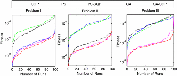
Fitness of 100 independent runs taken by five different algorithms
Fig. 6 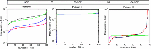
A graphical representation for 100 independent runs and MSE
Fig. 7 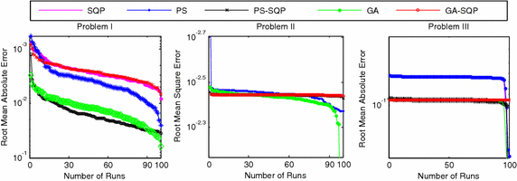
Fitness of 100 independent runs and RMAE for five different algorithms
Fig. 8 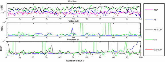
MSE against number of independent runs for each algorithm problem
-
The selection of appropriate number of neurons in the construction of ANN models has a significant role in the accuracy and complexity of the algorithms. The performance measuring indices bases on MAE, MSE, and RMAE are used to determine/evaluate the most suitable number of neurons in the proposed ANN models.
-
The histogram studies which show the relative frequency of obtaining performance indices values in certain range. Behavior of proposed methodologies through histogram plots are analyzed for all three problems


In order to evaluate small differences, we presented a statistical analysis, particularly fitting of normal distribution based on absolute errors (AEs) of SQP, PS and GA algorithms as shown in Figs. 9, 10 and 11 for problems I, II and III, respectively. The normal curve fitting is used to find how much the normal distribution accurately fits to AEs of our proposed results of algorithms with reported results as presented in Fig. 12. Figure 13 and 14 for problems I, II and III, respectively. In the Figs. 9, 10 and 11 also display 95 % confidence intervals (dotted curves) for the fitted normal distribution.

Normal distribution plot for Problem I for different results

Normal distribution plot for Problem II for different results

Normal distribution plot for Problem III for different results

Normality curve fitting of data for Problem I for different results

Normality curve fitting of data for Problem II for different results

Normality curve fitting of data for Problem II for different results
These confidence levels indicate that the performance of all six methods based on the fitted normal distribution and SQP showed higher accuracy than the other five in Problem I, in Problem II PS showed higher accuracy than the other five. But in the Problem III hybrid technique PS-SQP showed higher accuracy than the other five solvers.
It can be easily observed from these figures that, the result obtained by technique SQP in Problem I. PS in Problem II and hybrid PS-SQP in problem III is better than the results obtained by others algorithms. It is observed that for N = 30, our techniques show approximately better results from reported results and obtain the potential to minimize the errors.
Conclusions
In this research work, a detailed simulation process and statistical analysis of each case with multi-time independent test of each algorithm has been presented. Therefore, on the basis of these runs, we concluded the following important points.
-
The best advantage of the solver based on computational techniques with SQP, PS and GA algorithm to represent the approximate solution of Lane–Emden type differential equations as shown in Fig. 4.
-
The multi-runs of each algorithm independently provide a strong evidence for the accuracy of the proposed method.
-
The problem is still open for future work with the combination of different activation functions like Bessel’s polynomial and B-Polynomial etc.
-
The potential area of investigations to exploring in the existing numerical solver to deal with singularity along with strong nonlinear problems like nonlinear Lane–Emden equation based systems.
-
In future one may explore in Runge–Kutta numerical methods with adjusted boundary conditions as a promising future research direction in the domain of nonlinear singular systems for effective solution of Lane–Emden equation arising in astrophysics models for which relatively few solvers are available.
References
Ahmad I, Bilal M (2014) Numerical solution of Blasius equation through neural networks algorithm. Am J Comput Math 4:223–232. doi:10.4236/ajcm.2014.43019
Ahmad I, Mukhtar A (2015) Stochastic approach for the solution of multi-pantograph differential equation arising in cell-growth model. Appl Math Comput 261:360–372
Aleem A, Eldeen SH (2012) Optimal C-type passive filter based on minimization of the voltage harmonic distortion for nonlinear loads. IEEE Trans Ind Electron 59(1):281–289
Bazarghan M, Gupta R (2008) Automated classification of sloan digital sky survey (SDSS) stellar spectra using artificial neural networks. Astrophys Space Sci 315(1–4):201–210
Bora A, Gupta R, Singh HP, Murthy J, Mohan R, Duorah K (2008) A three-dimensional automated classification scheme for the TAUVEX data pipeline. Mon Not R Astron Soc 384(2):827–833
Bora A, Gupta R, Singh HP, Duorah K (2009) Automated star–galaxy segregation using spectral and integrated band data for TAUVEX/ASTROSAT satellite data pipeline. New Astron 14(8):649–653
Cantu-Paz E (2000) Efficient and accurate parallel genetic algorithms. Kluwer Academic, Boston
Chandrasekhar S (1967) Introduction to study of stellar structure. Dover Publications Inc., New York
Chowdhury MSH, Hashim I (2007a) Solutions of a class of singular second order initial value problems by homotopy-perturbation method. Phys Lett A 365:439–447
Chowdhury MSH, Hashim I (2007b) Solutions of Emden–Fowler equations by homotopy-perturbation method. Nonlinear Anal Real Word Appl 10:104–115
Datta BK (1996) Analytic solution to the Lane–Emden equation. Nuov Cim 111B:1385–1388
Davis HT (1962) Introduction to nonlinear differential and Integral equations. Dover Publications Inc., New York
Dehghan M, Shakeri F (2008) Approximate solution of a differential equation arising in astrophysics using the variational iteration method. New Astron 13:53–59
Demir H, Sungu IC (2009) Numerical solution of a class of nonlinear Emden–Fowler equations by using differential transformation method. J Arts Sci 12:75–81
Dolan ED, Lewis RM, Torczon V (2003) On the local convergence of pattern search”, SIAM. J Optim 14:567–583
Emden R (1907) Gaskugeln anwendungen der mechanischen Warmen-theorie auf kosmologie und meteorologische probleme. Teubner, Leipzig
Fowler RH (1914) The form near infinity of real continuous solutions of a certain differential equation of the second order. Q J Math (Oxford) 45:341–371
Fowler RH (1931) Further studies of Emden’s and similar differential equations. Quart. J. Math. (Oxf) 2:259–288
Govinder KS, Leach PGL (2007) Integrability analysis of the Emden–Fowler equation. J Nonlinear Math Phys 14:435–453
Gulati RK, Gupta R, Gothoskar P, Khobragade S (1994) Stellar spectral classification using automated schemes. Astrophys J 426:340–344
Gupta R, Singh HP, Volk K, Kwok S (2004). Automated classification of 2000 bright iras sources. Astrophys J Suppl Ser 152(2):201
Hercock RG (2003) Applied evolutionary algorithms in Java. Springer, New York
Hooke R, Jeeves TA (1996) Direct search solution of numerical and statistical problems. J Assoc Comput Mach 8(2):212–229
Khan JA, Raja MAZ, Rashidi MM, Syam MI, Wazwaz AM (2015) Nature-inspired computing approach for solving non-linear singular Emden–Fowler problem arising in electromagnetic theory. Connect Sci 27(04):377–396. doi:10.1080/09540091.2015.1092499
Kusano T, Manojlovic J (2011) Asymptotic behavior of positive solutions of sub linear differential equations of Emden–Fowler type. Comput Math Appl 62:551–565
Lane JH (1870) On the theoretical temperature of the sun under the hypothesis of a gaseous mass maintaining its volume by its internal heat and depending on the laws of gases known to terrestrial experiment. Am J Sci Arts Ser 2 4:57–74
Lewis R, Michael V, Torczon I (1999) Pattern search algorithms for bound con-strained minimization. SIAM J Optim 9(4):1082–1099
Lewis R, Michael V, Torczon I (2000) Pattern search methods for linearly constrained minimization. SIAM J Optim 10(3):917–941
Liao SJ (2003) A new analytic algorithm of Lane–Emden type equations. Appl Math Comput 142:1–16
Mall S, Chakraverty S (2014) Chebyshev neural network based model for solving Lane–Emden type equations. Appl Math Comput 247:100–114
Man FK, Tang KS, Wong S (1996) Genetic algorithms: concepts and applications [in engineering design]. IEEE Trans Ind Electron 43:519–534
Mellin CM, Mahomed FM, Leach PGL (1994) Solution of generalized Emden–Fowler equations with two symmetries. Int J Nonlinear Mech 29:529–538
Muatjetjeja B, Khalique CM (2001) Exact solutions of the generalized Lane–Emden equations of the first and second kind. Pramana 77:545–554
Nocedal J, Wright SJ (1999) Numerical optimization. Springer, New York
Raja MAZ (2014a) Unsupervised neural networks for solving Troesch’s problem. Chin Phys B 23(1):018903
Raja MAZ (2014b) Solution of the one-dimensional Bratu equation arising in the fuel ignition model using ANN optimised with PSO and SQP. Connect Sci 26(3):195–214. doi:10.1080/09540091.2014.907555
Raja MAZ (2014c) Stochastic numerical treatment for solving Troesch’s problem. Inf Sci 279:860–873
Raja MAZ (2014d) Numerical treatment for boundary value problems of Pantograph functional differential equation using computational intelligence algorithms. Appl Soft Comput J 24:806–821
Raja MAZ, Samar R (2014e) Numerical treatment of nonlinear MHD Jeffery–Hamel problems using stochastic algorithms. Comput Fluids 91:28–46
Raja MAZ, Khan JA, Haroon T (2015a) Stochastic Numerical treatment for thin film flow of third grade fluid using unsupervised neural networks. J Taiwan Inst Chem Eng 48:26–39. doi:10.1016/j.jtice.2014.10.018
Raja MAZ, Khan JA, Siddiqui AM, Behloul D, Haroon T, Samar R (2015b) Exactly satisfying initial conditions neural network models for numerical treatment of first Painlevé equation. Appl Soft Comput 26:244–256
Raja MAZ, Samar R, Haroon T, Shah SM (2015c) Unsupervised neural network model optimized with evolutionary computations for solving variants of nonlinear MHD Jeffery–Hamel problem. Appl Math Mech 36(12):1611–1638. doi:10.1007/s10483-015-2000-6
Raja MAZ, Ahmed I, Khan I, Syam MI, Wazwaz AM (2016a) Neuro-heuristic computational intelligence for solving nonlinear pantograph systems. Front Inf Technol Electron Eng (In press)
Raja MAZ, Khan MAR, Tariq M, Farooq U, Chaudhary NI (2016b) Design of bio-inspired computing technique for nanofluidics based on nonlinear Jeffery–Hamel flow equations. Can J Phys 94(5):474–489
Raja MAZ, Samar R, Alaidarous ES, Shivanian E (2016c) Bio-inspired computing platform for reliable solution of Bratu-type equations arising in the modeling of electrically conducting solids. Appl Math Model. 40(11): 5964–5977. doi:10.1016/j.apm.2016.01.034.
Raja MAZ, Shah FH, Ahad A, Khan NA (2016d) Design of bio-inspired computational intelligence technique for solving steady thin film flow of Johnson–Segalman fluid on vertical cylinder for drainage problem. Tiawan Inst Chem Eng. doi:10.1016/j.jtice.2015.10.020
Raja MAZ, Farooq U, Chaudhary NI, Wazwaz AM (2016e) Stochastic numerical solver for nanofluidic problems containing multi-walled carbon nanotubes. Appl Soft Comput 38:561–586. doi:10.1016/j.asoc.2015.10.015
Ramos JI (2005) Linearization techniques for singular initial-value problems of ordinary differential equations. Appl Math Comput 161:525–542
Rudd K, Ferrari S (2015) A constrained integration (CINT) approach to solving partial differential equations using artificial neural networks. Neurocomputing 155:277–285
Shukla HS, Tamsir M, Srivastava VK (2015) Numerical simulation of two dimensional sine-Gordon solitons using modified cubic B-spline differential quadrature method. AIP Adv 5:017121. doi:10.1063/1.4906256
Singh HP, Gulati RK, Gupta R (1998) Stellar spectral classification using principal component analysis and artificial neural networks. Mon Not R Astron Soc 295(2):312–318
Singh HP, Yuasa M, Yamamoto N, Gupta R (2006) Reliability checks on the Indo-Us stellar spectral library using artificial neural networks and principal component analysis. Publ Astron Soc Jpn 58(1):177–186
Singh OP, Pandey RK, Singh VK (2009) Analytical algorithm of Lane–Emden type equation arising in astrophysics using modified homotopy analysis method. Comput Phys Commun 180:1116–1124
Sivasubramani S, Swarup KS (2011) Sequential quadratic programming based differential evolution algorithm for optimal power flow problem. IET Gener Transm Distrib 5(11):1149–1154
Wazwaz AM (2001) A new algorithm for solving differential equation Lane–Emden type. Appl Math Comput 118:287–310
Wazwaz AM (2005) Adomian decomposition method for a reliable treatment of the Emden–Fowler equation. Appl Math Comput 161:543–560
Wazwaz AM (2006) The modified decomposition method for analytical treatment of differential equations. Appl Math Comput 173:165–176
Xu DY, Yang SL, Liu RP (2013) A mixture of HMM, GA, and Elman network for load prediction in cloud-oriented data centers. J Zhejiang Univ Sci C 14(11):845–858
Yu WC (1979) Positive basis and a class of direct search techniques, Sci Sin [Zhong-guoKexue] 1:53–68
Zhang YT, Liu CY, Wei SS, Wei CZ, Liu FF (2014) ECG quality assessment based on a kernel support vector machine and genetic algorithm with a feature matrix. J Zhejiang Univ Sci C 15(7):564–573
Authors’ contributions
IA has designed the main idea of mathematical modeling through neural networks with application of hybrid computational methods for the solutions of nonlinear singular Lane–Emden type differential equation arising in astrophysics models, moreover IA has contributed in conclusion. MAZR carried out the setting of tables and figures and has contributed in learning methodologies. He further contributed in manuscript darting. MB has contributed in data analysis for proposed problems and its performed the statistical analysis. FA carried out the results of proposed problems and performed the solvers and participated in the results and discussion section of the study. All authors read and approved the final manuscript.
Acknowledgements
The author would like to thank Siraj-ul-Islam Ahmad for valuable comments in this research work.
Competing interests
The authors declare that they have no competing interests.
Author information
Authors and Affiliations
Corresponding author
Appendix
Appendix
The necessary description of the routines used in the simulation studies are given for the ease of reproduction of the results. The software package of Matlab is used, in particularly Matlab optimization toolbox including ‘ga’ and ‘gaoptimset’ for Genetic algorithm, ‘patternsearch’ and ‘psoptimset’ for pattern search method, and ‘fmincon’ and ‘optimset’ for sequential quadratic programming algorithm. While the necessary coding for artificial neural network modeling of the equation, a good source of references is available in Matlab central file exchange server.
Rights and permissions
Open Access This article is distributed under the terms of the Creative Commons Attribution 4.0 International License (http://creativecommons.org/licenses/by/4.0/), which permits unrestricted use, distribution, and reproduction in any medium, provided you give appropriate credit to the original author(s) and the source, provide a link to the Creative Commons license, and indicate if changes were made.
About this article

Cite this article
Ahmad, I., Raja, M.A.Z., Bilal, M. et al. Bio-inspired computational heuristics to study Lane–Emden systems arising in astrophysics model. SpringerPlus 5, 1866 (2016). https://doi.org/10.1186/s40064-016-3517-2
Received:
Accepted:
Published:
DOI: https://doi.org/10.1186/s40064-016-3517-2