
Abstract
In this paper, we present the monotonicity analysis for the nabla fractional differences with discrete generalized Mittag-Leffler kernels \(( {}^{ABR}_{a-1}{\nabla }^{\delta ,\gamma }y )(\eta )\) of order \(0<\delta <0.5\), \(\beta =1\), \(0<\gamma \leq 1\) starting at \(a-1\). If \(({}^{ABR}_{a-1}{\nabla }^{\delta ,\gamma }y ) ( \eta )\geq 0\), then we deduce that \(y(\eta )\) is \(\delta ^{2}\gamma \)-increasing. That is, \(y(\eta +1)\geq \delta ^{2} \gamma y(\eta )\) for each \(\eta \in \mathcal{N}_{a}:=\{a,a+1,\ldots\}\). Conversely, if \(y(\eta )\) is increasing with \(y(a)\geq 0\), then we deduce that \(({}^{ABR}_{a-1}{\nabla }^{\delta ,\gamma }y )(\eta ) \geq 0\). Furthermore, the monotonicity properties of the Caputo and right fractional differences are concluded to. Finally, we find a fractional difference version of the mean value theorem as an application of our results. One can see that our results cover some existing results in the literature.
1 Introduction
In the past two decades, fractional calculus and its applications have been applied into various fields due to its accurate describing in many scientific fields, such as fractional stochastic noise [1], fraction order memristive chaotic circuits [2], fractional order financial models [3], and fractional order relaxation–oscillation models [4]. Also, it has wide application in various research areas, which one can find in the references [5–13].
Along the years, fractional calculus has attracted more and more researchers’ attention and has found applications in several fields of engineering and the applied sciences (see [5–8]). Recently, many fractional models were proposed showing the significance of fractional calculus. Discrete fractional calculus can be seen as the most recent model of fractional calculus which has been widely used.
Recently, discrete fractional calculus gains a great deal of interest by many researchers. In [14, 15], the authors introduced the discrete fractional sums and differences which produced directly from the Riemann–Liouville (RL) fractional integrals and derivatives, respectively. To review the history of discrete fractional operators, their properties and information related to discrete fractional calculus applications one can refer to [16–22] and the references therein. Nowadays, being new fractional integral and derivative operators make the researchers attempt to introduce a new definition of discrete fractional sum and difference operators corresponding to them. Those models are receiving the attention of many researchers (see [23–26]).
Monotonocity analysis has become very important in discrete fractional calculus which was firstly applied for the discrete fractional operators of RL version by Atici and Uyanik in [27]. In [28], the authors found the monotonicity analysis for the Caputo–Fabrizo (CF) version of discrete fractional operators. In [29], the monotonicity analysis for the Atangana–Baleanu (AB) version of discrete fractional operators with discrete Mittag-Leffler (ML) kernels was done. In addition, the monotonicity analysis has been established for the h-discrete fractional operators in [30, 31] (see also [32]).
However, to the best of our knowledge so far, the monotonicity results have not been considered for the discrete fractional operators with discrete generalized ML kernels [33]. Therefore, our aim in this article is to establish the monotonicity analysis for the above model of discrete fractional operators that can cover the monotonicity results in [29].
The structure of the article is designed as follows: Sect. 2.1 deals with recalling the RL-fractional sums and generalized discrete ML functions. Section 2.2 deals with recalling the generalized discrete AB fractional operators with their equivalent formulas and definition of δ-monotonicity. In Sect. 3 we discuss the monotonicity analysis for the 2-parameter fractional difference operators involving the discrete generalized ML kernels. Section 4 deals with the application of our findings on the mean value theorem, and in Sect. 5 we conclude the article.
2 Preliminaries
This section deals with some basic concepts on discrete fractional operators and discrete ML functions.
2.1 RL-fractional sums and generalized ML function
Definition 2.1
The ℓ increasing factorial function of η is given by
Generally, the increasing factorial function is given by
for \(\eta \in \mathcal{R}\setminus \{\ldots ,-2,-1,0\}\), where \(\mathcal{R}\) denotes the set of real numbers.
Definition 2.2
Let the backward jump operator be given by \(\rho (s)=r-1\). Then, for any function \(f:\mathcal{N}_{a}\to \mathcal{R}\), the nabla left fractional sum of order \(\delta >0\) in the sense of RL is defined by
Also, for any function \(f: _{b}\mathcal{N}=\{b,b-1,b-2,\ldots\}\to \mathcal{R}\), the nabla right fractional sum of order \(\delta >0\) in the sense of RL is defined by
Lemma 2.1
For any \(a, b\in \mathcal{R}\) and \(\delta _{1}, \delta _{2}>0\), we have
Lemma 2.2
For any \(\delta _{1}, \delta _{2}\in \mathcal{R}\) and any f defined on \(\mathcal{N}_{a}\), we have
Lemma 2.3
([25])
Let f be defined on \(\mathcal{N}_{a}\), then, for any \(0<\delta <1\), we have
The nabla discrete ML functions are important; they are recalled now.
Definition 2.3
([33])
For any \(\lambda \in \mathcal{R}\) and \(\delta , \beta , \gamma , \eta \in \mathbb{C}\) with \(\operatorname {Re}(\delta )>0\), the nabla discrete generalized ML function is defined by
where \((\gamma )_{\ell }=\gamma (\gamma +1)\cdots (\gamma +\ell -1)\) is the Pochhammer symbol. Specifically, if \(\gamma =1\), we get the nabla discrete two parameters ML function:
And if \(\beta =\gamma =1\), we get the nabla discrete one parameter ML function:
Lemma 2.4
([33])
For any \(\delta >0\), \(\beta >-1\), \(\gamma , \eta \in \mathbb{C}\) and \(\lambda \in \mathcal{R}\) with \(|\lambda |<1\), we have
Remark 2.1
-
(i)
For any \(\lambda =-\frac{\delta }{1-\delta }\), \(0<\delta <\frac{1}{2}\), \(\eta \in \mathcal{N}\) and \(0<\gamma \leq 1\), the two parameters ML function \(\mathrm{E}_{\overline{{\delta ,1}}}^{\gamma }(\lambda ,\eta )\) is monotonically decreasing. Here, we find some initial values of \(\mathrm{E}_{\overline{{\delta ,1}}}^{\gamma }(\lambda ,\eta )\):
-
\(\mathrm{E}_{\overline{{\delta ,1}}}^{\gamma }(\lambda ,0)=1\).
-
\(\mathrm{E}_{\overline{{\delta ,1}}}^{\gamma }(\lambda ,1)=(1-\delta )^{ \gamma }\).
-
\(\mathrm{E}_{\overline{{\delta ,1}}}^{\gamma }(\lambda ,2)=(1-\delta )^{ \gamma } (1-\delta ^{2}\gamma )\).
-
\(\mathrm{E}_{\overline{{\delta ,1}}}^{\gamma }(\lambda ,3)= \frac{(1-\delta )^{\gamma }}{2} (\delta ^{4}\gamma (\gamma +1)- \delta ^{3}\gamma -3\delta ^{2}\gamma +2 )\).
On the other hand, the Figure 1 can confirm the validity of the above results.
Figure 1 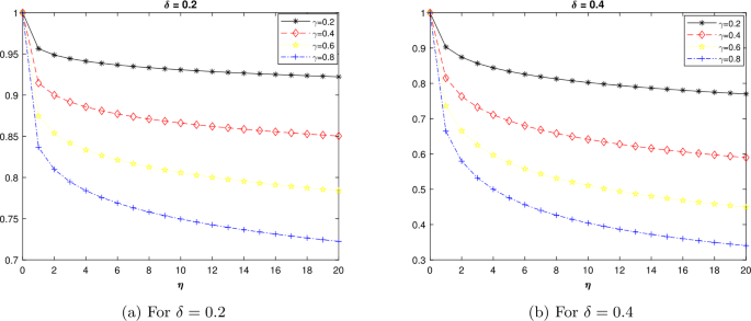
Plot of \(\mathrm{E}_{\overline{{\delta ,1}}}^{\gamma }(\lambda ,\eta )\) for different values of γ
-
-
(ii)
From (i) and Definition 2.3, we have
$$\begin{aligned} \nabla \mathrm{E}_{\overline{{\delta ,1}}}^{\gamma }(\lambda , \eta ) &= \sum_{k=0}^{\infty }\lambda ^{k} \frac{k\delta \eta ^{\overline{k\delta -1}}(\gamma )_{k}}{\Gamma (k\delta +1)k!} =\sum_{k=1}^{\infty } \lambda ^{k} \frac{\eta ^{\overline{k\delta -1}}(\gamma )_{k}}{\Gamma (k\delta )k!} \\ &=\lambda \sum_{k=0}^{\infty }\lambda ^{k} \frac{\eta ^{\overline{k\delta +\delta -1}}(\gamma )_{k+1}}{\Gamma (k\delta +\delta )(k+1)!} :=\lambda \mathbf{E}_{\overline{{\delta }}}^{\gamma }( \lambda , \eta )< 0. \end{aligned}$$(2.7)

This implies that \(\mathbf{E}_{\overline{{\delta }}}^{\gamma }(\lambda ,\eta )\) is strictly positive for \(\lambda <0\).
Proof
In proving (i), we need the following identity:
□
2.2 Generalized discrete ABR and ABC and monotonicity definitions
The discrete ABR and ABC fractional differences and sums were introduced in [24] using the one parameter discrete ML function. After that, the generalized discrete ABR and ABC fractional differences and sums were introduced by Abdeljawad in [33] using the generalized discrete ML function:
Definition 2.4
([33])
Let \(\lambda =-\frac{\delta }{1-\delta }\) and \(0<\delta <1/2\). Then, for \(\gamma \in \mathcal{R}\) and \(\operatorname {Re}(\beta )>0\), the left generalized discrete ABR fractional difference is defined by
and the right generalized discrete ABR fractional difference is defined by
Also, the left generalized discrete ABC fractional difference is defined by
and the right generalized discrete ABC fractional difference is defined by
where \(B(\delta )\) is a multiplier and it satisfies \(B(0)=B(1)=1\).
In this article, we consider a specific case where \(0<\gamma \leq 1\) and \(\beta =1\). Then we can rewrite the above definitions as follows.
Definition 2.5
Let \(\lambda =-\frac{\delta }{1-\delta }\), \(0<\delta <1/2\) and \(0<\gamma \leq 1\). Then the left 2-parameter discrete ABR fractional difference is defined by
and the right 2-parameter discrete ABR fractional difference is defined by
Also, the left 2-parameter discrete ABC fractional difference is defined by
and the right 2-parameter discrete ABC fractional difference is defined by
Theorem 2.1
([33])
Let y be defined on \(\mathcal{N}_{a}\) with \(b \equiv a \pmod{1}\), then, for any \(\lambda =-\frac{\delta }{1-\delta }\), \(0<\delta <1/2\), \(\gamma \in \mathcal{R}\) and \(0<\operatorname {Re}(\beta )<1\), we have the following relationships between the discrete ABC and discrete ABR fractional differences:
in the left-side sense and
in the right-side sense.
Definition 2.6
([33])
y be defined on \(\mathcal{N}_{a}\) and \(a \equiv b \pmod{1}\). Then the left generalized AB fractional sum of order \(0<\delta \leq 1\), \(\beta >0\), \(\gamma >0\) is defined by
Theorem 2.2
([33])
Let y be defined on \(\mathcal{N}_{a}\) with \(b \equiv a \pmod{1}\), then, for any \(\lambda =-\frac{\delta }{1-\delta }\), \(0<\delta <1/2\) and \(\gamma , \beta \in \mathbb{Z}\), we have
Now, we recall the monotonicity definitions.
Definition 2.7
Let \(y:\mathcal{N}_{a}\to \mathcal{R}\) be a function satisfying \(y(a)\geq 0\). Then y is called a δ-increasing function on \(\mathcal{N}_{a}\), if
Observe that, if \(y(\eta )\) is increasing on \(\mathcal{N}_{a}\), then \(y(\eta +1)\geq y(\eta )\) for all \(\eta \in \mathcal{N}_{a}\), and thus \(y(\eta )\) is δ-increasing on \(\mathcal{N}_{a}\).
Definition 2.8
Let \(y:\mathcal{N}_{a}\to \mathcal{R}\) be a function satisfying \(y(a)\leq 0\). Then y is called a δ-decreasing function on \(\mathcal{N}_{a}\), if
Observe that, if \(y(\eta )\) is decreasing on \(\mathcal{N}_{a}\), then \(y(\eta +1)\leq y(\eta )\) for all \(\eta \in \mathcal{N}_{a}\), and thus \(y(\eta )\) is δ-decreasing on \(\mathcal{N}_{a}\).
Remark 2.2
Note that, if \(\delta =1\) in Definition 2.7, then the increasing and δ-increasing concepts coincide, and if \(\delta =1\) in Definition 2.8, then the decreasing and δ-decreasing concepts coincide.
3 Difference monotonicity outlines
Theorem 3.1
Let \(y:\mathcal{N}_{a-1}\to \mathcal{R}\) be a function. Suppose that, for \(0<\delta <\frac{1}{2}\) and \(0<\gamma \leq 1\), we have
then \(y(\eta )\) is \(\delta ^{2}\gamma \)-increasing.
Proof
Rewrite \(({}^{ABR}_{a-1}{\nabla }^{\delta ,\gamma }y )(\eta )= \frac{B(\delta )}{1-\delta }\nabla S(\eta )\), where \(S(\eta )=\sum_{s=a}^{\eta }y(s)\mathrm{E}_{\overline{{\delta ,1}}}^{ \gamma }(\lambda ,\eta -\rho (s))\). From assumption and since \(\mathrm{E}_{\overline{{\delta ,1}}}^{\gamma }(\lambda ,1)=1\), we have
Then we proceed with our proof by induction. First, if we substitute \(\eta =a\) in (3.1), we deduce that \(y(a)\geq 0\). If we substitute \(\eta =a+1\) in (3.1), then, in view of Remark 2.1, we can deduce
Now, we assume that
and we have to show that \(y(a+k+1)\geq \delta ^{2}\gamma y(a+k)\). By substituting \(\eta =a+k+1\) in (3.1) and then using Eq. (2.7), we find that
Then, by using Eq. (2.7) and Remark 2.1, it follows that
This completes the proof. □
Theorem 3.2
Let \(y:\mathcal{N}_{a-1}\to \mathcal{R}\) be a function. Suppose that, for \(0<\delta <\frac{1}{2}\) and \(0<\gamma \leq 1\), we have
then \(y(\eta )\) is \(\delta ^{2}\gamma \)-decreasing.
Proof
The proof is similar to Theorem 3.1. □
Corollary 3.1
Let \(y:\mathcal{N}_{a-1}\to \mathcal{R}\) be a function. Suppose that, for \(0<\delta <\frac{1}{2}\) and \(0<\gamma \leq 1\), we have
then \(y(\eta )\) is \(\delta ^{2}\gamma \)-increasing.
Proof
The proof follows directly from Theorem 3.1 and Theorem 2.1 with \(\beta =1\). □
Corollary 3.2
Let \(y:\mathcal{N}_{a-1}\to \mathcal{R}\) be a function. Suppose that, for \(0<\delta <\frac{1}{2}\) and \(0<\gamma \leq 1\), we have
then \(y(\eta )\) is \(\delta ^{2}\gamma \)-decreasing.
Proof
The proof follows directly from Theorem 3.2 and Theorem 2.1 with \(\beta =1\). □
Remark 3.1
If we take \(\gamma =1\) in Theorem 3.1, Theorem 3.2 and Corollary 3.1, then we get Theorem 2, Theorem 6 and Theorem 3 in [29], respectively.
Theorem 3.3
Let \(y:\mathcal{N}_{a-1}\to \mathcal{R}\) be a function satisfying \(y(a)\geq 0\) and let \(y(\eta )\) be increasing on \(\mathcal{N}_{a}\). Then, for \(0<\delta <\frac{1}{2}\) and \(0<\gamma \leq 1\), we have
Proof
It is enough to show that \(S(\eta )\) is increasing, where \(S(\eta )\) is given in Theorem 3.1. By substituting \(\eta =a\) in (3.1) and making use of the assumption, we deduce that
Suppose that \(S(k)-S(k-1)\geq 0\) for any \(k< t\), then we have to show that \(S(\eta )-S(\eta -1)\geq 0\). Since \(y(\eta )\) is an increasing function, we have \(y(\eta )\geq y(\eta -1)\geq y(a)\geq 0\) for each \(\eta \in \mathcal{N}_{a}\). Then, from (3.1), we have
Since \((1-\delta )^{\gamma }>0\) and \(y(\eta )\geq y(\eta -1)\), we have
Then, by using this in (3.2), we get
which we can rearrange to get the desired result. □
The following theorems are similar to Theorem 3.3.
Theorem 3.4
Let \(y:\mathcal{N}_{a-1}\to \mathcal{R}\) be a function satisfying \(y(a)>0\) and let \(y(\eta )\) be strictly increasing on \(\mathcal{N}_{a}\). Then, for \(0<\delta <\frac{1}{2}\) and \(0<\gamma \leq 1\), we have
Theorem 3.5
Let \(y:\mathcal{N}_{a-1}\to \mathcal{R}\) be a function satisfying \(y(a)\leq 0\) and let \(y(\eta )\) be decreasing on \(\mathcal{N}_{a}\). Then, for \(0<\delta <\frac{1}{2}\) and \(0<\gamma \leq 1\), we have
Theorem 3.6
Let \(y:\mathcal{N}_{a-1}\to \mathcal{R}\) be a function satisfying \(y(a)\leq 0\) and let \(y(\eta )\) be strictly decreasing on \(\mathcal{N}_{a}\). Then, for \(0<\delta <\frac{1}{2}\) and \(0<\gamma \leq 1\), we have
Remark 3.2
If we take \(\gamma =1\) in Theorems 3.3–3.5, then we get Theorem 4, Theorem 5 and Theorem 7 in [29], respectively.
4 MVT application
This section deals with the application of our results to the mean value theorem (MVT). First, we need the following lemmas.
Lemma 4.1
For any \(0<\delta <\frac{1}{2}\) and \(0<\gamma \leq 1\) and \(\eta \in \mathcal{N}_{a}\), we have
for each \(k=1, 2,\ldots \) .
Proof
By applying Lemma 2.3 for \(f(\eta )=\mathrm{E}_{\overline{{\delta ,1}}}^{\gamma }(\lambda ,\eta -a+1)\), we get
where we used \(\mathrm{E}_{\overline{{\delta ,1}}}^{\gamma }(\lambda ,1)=(1-\delta )^{ \gamma }\).
On the other hand, from the definition of discrete nabla fractional sum, we have
For \(y(\eta )=\mathrm{E}_{\overline{{\delta ,1}}}^{\gamma }(\lambda ,\eta -a+1)\), it follows that
By taking ∇ to both sides of (4.3), we obtain
By using (4.4) in (4.2), we obtain
which completes the proof. □
Lemma 4.2
For any \(\delta , \gamma \in \mathbb{C}\), we have
Proof
The proof follows directly from [33, Example 1] and the fact that \(\mathrm{E}_{\overline{{\delta ,1}}}^{0}(\lambda , \eta -a)=1\). □
Remark 4.1
By using the relationship between the gamma functions
we can obtain the following relationship between the combination formula and the Pochhammer symbol:
This is a useful tool in the proof of the next theorem.
Now, from [33], we see that
One can note that Eq. (4.5) does not contain \(y(a)\). However, the next result contains an initial value \(y(a)\) which will be a great tool to prove our fractional difference MVT.
Theorem 4.1
Let y be a function defined on \(\mathcal{N}_{a-1}\), then, for \(0<\delta <\frac{1}{2}\) and \(0<\gamma \leq 1\), we have
Proof
From the definition (2.8) with \(\beta =1\), we have
Then, by using the series formula (2.18) with \(\beta =1\), Lemma 4.1 and Remark 4.1, we can deduce
Then, by using the series formula (2.19) and Lemma 4.3, it follows that
which completes the required result. □
Remark 4.2
If we put \(\gamma =1\) in Theorem 4.1, we directly obtain Theorem 8 in [29].
Proof
From (4.6), we have for \(\gamma =1\)
where the fact \((-1)_{k}=0\), \(k\geq 2\) is used. □
Now, let \(R(\delta ,\eta ,a)= \frac{\delta \gamma (1-\delta )^{\gamma -1}(\eta -a+1)^{\overline{\delta -1}}}{\Gamma (\delta )} +(1-\delta )^{\gamma }\sum_{k=2}^{\infty }\lambda ^{k} \frac{(-\gamma )_{k}}{k!} \frac{(\eta -a+1)^{\overline{\delta k-1}}}{\Gamma (\delta k)}\), then it is clear that \(R(\delta ,\eta ,a)<1\).
Lemma 4.3
Let g be a strictly increasing function defined on \(\mathcal{N}_{a}\). Then, for any \(0<\delta <\frac{1}{2}\), \(0<\gamma \leq 1\), we have
Proof
Since g is strictly increasing, by using Theorem 3.4, we have
Applying \({}^{AB}_{a}{\nabla }^{-(\delta ,\gamma )}\) to both sides of the above inequality we get
Considering \(({}^{AB}_{a}{\nabla }^{-(\delta ,\gamma )} {}^{ABR}_{a-1}{\nabla }^{\delta ,\gamma }g )(\eta )=g(b)-R( \delta ,\eta ,a)g(a)\) (by using Theorem 4.1), the proof follows. □
Then we can deduce the following MVT.
Theorem 4.2
(MVT)
Suppose that f and g are two functions defined on \(\mathcal{N}_{a,b}:=\{a,a+1,a+2,\ldots,b\}\) with \(a \equiv b \pmod{1}\), g is a strictly increasing and \(0<\delta <\frac{1}{2}\), \(0<\gamma \leq 1\). Then there exist \(s_{1}, s_{2}\in \mathcal{N}_{a,b}\) such that
Proof
On the contrary, we suppose that (4.7) is not true. Then either
or
With the help of Lemma 4.3, we see that \(g(b)-R(\delta ,b,a)g(a)>0\). Also, by assumption g is strictly increasing and hence \(({}^{ABR}_{a-1}{\nabla }^{\delta ,\gamma }g )(\eta )>0\) by Theorem 3.4. Therefore, inequality (4.8) can be written in the following form:
By applying the fractional sum operator (evaluated at \(\eta =b\)) to both sides of (4.10) and by making use of Theorem 4.1, we can deduce
which is a contradiction. By using the same method as used for (4.8), we can conclude that (4.9) will be a contradiction. Thus the proof is completed. □
5 Conclusion
The results of the article can be summarized as follows:
-
First, we have recalled the RL-fractional sums, generalized discrete ML function, and the generalized discrete AB fractional operators with their equivalent formulas. Also, the definition of δ-monotonicity has been recalled.
-
We have considered the monotonicity analysis for the nabla fractional difference operator with discrete generalized ML kernel \(({}^{ABR}_{a-1}{\nabla }^{\delta ,\gamma }y )(\eta )\) of order \(0<\delta <0.5\), \(0<\gamma \leq 1\) starting at \(a-1\).
-
If \(({}^{ABR}_{a-1}{\nabla }^{\delta ,\gamma }y )(\eta ) \geq 0\), then we have deduced that \(y(\eta )\) is \(\delta ^{2}\gamma \)-increasing. That is \(y(\eta +1)\geq \delta ^{2}y(\eta )\) for each \(\eta \in \mathcal{N}_{a}\).
-
If \(y(\eta )\) is increasing and \(y(a)\geq 0\), then we have concluded that \(({}^{ABR}_{a-1}{\nabla }^{\delta ,\gamma }y )(\eta ) \geq 0\).
-
Monotonicity results for the nabla Caputo fractional difference with discrete generalized ML kernel have been found as well.
-
Our results can be seen as the generalization of the results in [29].
-
Additionally, we have established a new version of the MVT in the frame fractional differences in the setting of generalized AB.
-
In the case of the case \(h\mathbb{Z}\) in the setting of discrete ML-kernel (AB) [30] and discrete exponential kernel [34], it was noticed that the monotonicity factor depends on the step h. However, for the discrete power law case [31] the monotonicity factor is independent of the step h. Since our results in this article generalize those in [29], it is of interest to generalize the results in this article for the \(h\mathbb{Z}\) case so that the monotonicity factor will depend on δ, γ, and h!
-
We have been able to address the monotonicity analysis for the ML kernels with parameters \(0<\delta <0.5\), \(\beta =1\), and \(0<\gamma \leq 1\). Is it possible to register homogeneous monotonicity properties on certain discrete intervals for the case when \(\beta \neq 1\)?
-
In Remark 2.1, we described the decreasing behavior of the discrete ML functions of order \(0<\delta <0.5\), \(\beta =1\), and \(0<\gamma \leq 1\) by calculating the first 4 terms and by providing graphs. However, the proof of this behavior analytically is still open!
Availability of data and materials
Not applicable.
References
Cottone, G., Paola, M.D., Santoro, R.: A novel exact representation of stationary colored Gaussian processes (fractional differential approach). J. Phys. A, Math. Theor. 43(8), Article ID 085002 (2010)
Meng, F., Zeng, X., Wang, Z.: Impulsive anti-synchronization control for fractional-order chaotic circuit with memristor. Indian J. Phys. 93(9), 1187–1194 (2019)
Xu, C.-J., Liao, M.-X., Li, P.-L., Xiao, Q.-M., Yuan, S.: PD9 control strategy for a fractional-order chaotic financial model. Complexity 2019, Article ID 2989204 (2019)
Mainardi, F.: Fractional relaxation-oscillation and fractional diffusion-wave phenomena. Chaos Solitons Fractals 7(9), 1461–1477 (1996)
Miller, K.S., Ross, B.: An Introduction to the Fractional Calculus and Fractional Differential Equations. Wiley, New York (1993)
AbuArqub, O., Maayah, B.: Numerical solutions of integrodifferential equations of Fredholm operator type in the sense of the Atangana–Baleanu fractional operator. Chaos Solitons Fractals 117, 117–124 (2018)
Kilbas, A.A., Srivastava, H.M., Trujillo, J.J.: Theory and Applications of Fractional Differential Equations. North-Holland Mathematical Studies, vol. 204. Elsevier, Amsterdam (2006)
Diethelm, K.: The Analysis of Fractional Differential Equations. Springer, Berlin (2010)
AbuArqub, O., Maayah, B.: Modulation of reproducing kernel Hilbert space method for numerical solutions of Riccati and Bernoulli equations in the Atangana–Baleanu fractional sense. Chaos Solitons Fractals 125, 163–170 (2019)
Tarasov, V.: Handbook of Fractional Calculus with Applications, Applications in Physics, Part A, vol. 4. de Gruyter, Berlin (2019)
Srivastava, H.M., Mohammed, P.O., Guirao, J.L.G., Hamed, Y.S.: Some higher-degree Lacunary fractional splines in the approximation of fractional differential equations. Symmetry 422(13), 1–13 (2021)
Martinez, M., Mohammed, P.O., Valdes, J.E.N.: Non-conformable fractional Laplace transform. Kragujev. J. Math. 46(3), 341–354 (2022)
Srivastava, H.M.: Fractional-order derivatives and integrals: introductory overview and recent developments’. Kyungpook Math. J. 60, 73–116 (2020)
Gray, H.L., Zhang, N.-F.: On a new definition of the fractional difference. Math. Comput. 50(182), 513–529 (1988)
Miller, K.S., Ross, B.: Fractional difference calculus. In: Proceedings of the International Symposium on Univalent Functions, Fractional Calculus and Their Applications, pp. 139–152. Nihon University, Koriyama (1989)
Atici, F., Eloe, P.: A transform method in discrete fractional calculus. Int. J. Difference Equ. 2(2), 165–176 (2007)
Atici, F., Eloe, P.: Initial value problems in discrete fractional calculus. Proc. Am. Math. Soc. 137, 981–989 (2009)
Srivastava, H.M., Mohammed, P.O.: A correlation between solutions of uncertain fractional forward difference equations and their paths. Front. Phys. 8, 280 (2020)
Goodrich, C., Peterson, A.C.: Discrete Fractional Calculus. Springer, Berlin (2015)
Goodrich, C.: Existence of a positive solution to a system of discrete fractional boundary value problems. Appl. Math. Comput. 217, 4740–4753 (2011)
Mohammed, P.O.: A generalized uncertain fractional forward difference equations of Riemann–Liouville type. J. Math. Res. 11(4), 43–50 (2019)
Abdeljawad, T.: Dual identities in fractional difference calculus within Riemann. Adv. Differ. Equ. 2017, 36 (2017)
Abdeljawad, T.: On delta and nabla Caputo fractional differences and dual identities. Discrete Dyn. Nat. Soc. 2013, 12 (2013)
Abdeljawad, T., Baleanu, D.: Discrete fractional differences with nonsingular discrete Mittag-Leffler kernels. Adv. Differ. Equ. 2016, 232 (2016)
Abdeljawad, T.: Different type kernel h-fractional differences and their fractional h-sums. Chaos Solitons Fractals 116, 146–156 (2018)
Abdeljawad, T., Al-Mdallal, Q.M.: Discrete Mittag-Leffler kernel type fractional difference initial value problems and Gronwall’s inequality. J. Comput. Appl. Math. 339, 218–230 (2018)
Atici, F., Uyanik, M.: Analysis of discrete fractional operators. Appl. Anal. Discrete Math. 9, 139–149 (2015)
Abdeljawad, T., Baleanu, D.: On fractional derivatives with exponential kernel and their discrete versions. Rep. Math. Phys. 80(1), 11–27 (2017)
Abdeljawad, T., Baleanu, D.: Monotonicity analysis of a nabla discrete fractional operator with discrete Mittag-Leffler kernel. Chaos Solitons Fractals 102, 106–110 (2017)
Suwan, I., Abdeljawad, T., Jarad, F.: Monotonicity analysis for nabla h-discrete fractional Atangana–Baleanu differences. Chaos Solitons Fractals 117, 50–59 (2018)
Suwan, I., Owies, S., Abdeljawad, T.: Monotonicity results for h-discrete fractional operators and application. Adv. Differ. Equ. 2018, 207 (2018)
Ghanbari, B., Günerhan, H., Srivastava, H.M.: An application of the Atangana–Baleanu fractional derivative in mathematical biology: a three-species predator-prey model. Chaos Solitons Fractals 138, Article ID 109919 (2020)
Abdeljawad, T.: Fractional difference operators with discrete generalized Mittag-Leffler kernels. Chaos Solitons Fractals 126, 315–324 (2019)
Suwan, I., Owies, S., Abdeljawad, T.: Fractional h-differences with exponential kernels and their monotonicity properties (2020). https://doi.org/10.1002/mma.6213
Acknowledgements
The last author would like to thank Prince Sultan University for funding this work through research group Nonlinear Analysis Methods in Applied Mathematics (NAMAM) group number RG-DES-2017-01-17.
Funding
Not applicable.
Author information
Authors and Affiliations
Contributions
All authors contributed equally and significantly in writing this article. All authors read and approved the final manuscript.
Corresponding authors
Ethics declarations
Competing interests
The authors declare that they have no competing interests.
Consent for publication
Not applicable.
Rights and permissions
Open Access This article is licensed under a Creative Commons Attribution 4.0 International License, which permits use, sharing, adaptation, distribution and reproduction in any medium or format, as long as you give appropriate credit to the original author(s) and the source, provide a link to the Creative Commons licence, and indicate if changes were made. The images or other third party material in this article are included in the article’s Creative Commons licence, unless indicated otherwise in a credit line to the material. If material is not included in the article’s Creative Commons licence and your intended use is not permitted by statutory regulation or exceeds the permitted use, you will need to obtain permission directly from the copyright holder. To view a copy of this licence, visit http://creativecommons.org/licenses/by/4.0/.
About this article

Cite this article
Mohammed, P.O., Hamasalh, F.K. & Abdeljawad, T. Difference monotonicity analysis on discrete fractional operators with discrete generalized Mittag-Leffler kernels. Adv Differ Equ 2021, 213 (2021). https://doi.org/10.1186/s13662-021-03372-2
Received:
Accepted:
Published:
DOI: https://doi.org/10.1186/s13662-021-03372-2