
Abstract
We attempt to motivate utilization of some local derivatives of arbitrary orders in clinical medicine. For this purpose, we provide two efficient solution methods for various problems that occur in nature by employing the local proportional derivative defined by the proportional derivative (PD) controller. Under some necessary assumptions, a detailed exposition of the instantaneous volume in a lung is furnished by conformable derivative and such modified conformable derivatives as truncated M-derivative and proportional derivative. Moreover, we wish to investigate the performance of the above-mentioned operators in applications by plotting several graphs of the governing equations.
1 Introduction
In medicine, mechanical ventilation (assisted ventilation) is a supportive treatment provided by a medical machine named a ventilator. This breathing machine is utilized for severe illnesses in an intensive care unit (ICU) in case of breathing failure, coma, neuromuscular disorders, acute severe asthma, and so on. It is also used to get rid of carbon dioxide to supply oxygen into the lungs, to facilitate breathing, or to breathe for critically ill patients. Differently from the many specific types of mechanical ventilation, there are two main mechanical ventilations involving positive pressure ventilation and negative pressure ventilation. The former pushes air or gas into the lungs, and the latter sucks air into the lungs by stimulating chest movement. The ventilator is connected to the patient by a tube in windpipe through the nose or mouth and blows air plus oxygen needed into the patient’s lung. Also, positive end-expiratory pressure (PEEP) can be provided by a ventilator, which helps to hold the lungs open to prevent the air sacs from collapsing. Patients on a ventilator providing more oxygen than other devices like masks are monitored to control the respiratory rate, heart rate, oxygen saturation, and blood pressure. Besides the benefits of using a ventilator, there are also some risks. The ventilator itself is not a method of treatment, it only ensures support until the patient feels better or heals. Moreover, people on ventilators cannot talk or eat, and some are uncomfortable with a tube (endotracheal or ET tube) in their nose or mouth. It can cause an infection like pneumonia because the tube allows bacteria to easily get into the person’s lung. Occasionally, the lung may collapse owing to getting full of air, and in addition to this, lung damage, side effects of medications, inability to discontinue ventilator support, and alveolar damage can be regarded among the risks of the ventilator. Hence the health care team all the time tries to help a patient get rid of the ventilator as soon as possible.
This study is intended to observe the model of the mechanical process of a ventilator as appeared in [1]. Some assumptions must be made for this process of filling the lungs with air and letting them deflate to some volume. The lung is modeled by a single compartment. The ventilator applies a constant pressure \(P_{d}\) to the airway, and it is zero during expiration. Each breath length is fixed by \(t_{b}\) determined by the clinician, and \(t_{j}\) denotes the inspiratory time. The pressure of the ventilator is denoted by \(P_{d}\). Additionally, the pressure balance at the airway is presented by
where \(P_{l}\) stands for airway-resistance drop, \(P_{k}\) is the lung elastic pressure, \(P_{m}\) is the residual pressure, and the pressure applied to airway is denoted by \(P_{aw}\). In addition, \(P_{m}\) can be computed by the condition \(\mathcal{V}_{e}(t_{b})=0\) as given in the following formula:
Furthermore, the mean alveolar pressure, which is the average pressure in the lung during inspiration, is calculated by the condition \(\mathcal{V}_{i}(0)=0\) as follows:
Under the assumptions above and by utilizing the pressure equation (1), a model for the instantaneous volume in a lung is presented by
where \(\mathcal{V}_{i}(t)\) is the volume during inspiration, \(\mathcal{V}_{e}(t)\) denotes the volume during expiration, and \(\mathcal{V}_{T}\) stands for the tidal volume of the breath. It is assumed that \(P_{l}\) is proportional to the flows into and out of the lung and \(P_{k}\) is proportional to the instantaneous volume of the lung; that is, \(P_{l}=R (\frac{d\mathcal{V}(t)}{dt} )\) and \(P_{k}= (\frac{1}{C} )\mathcal{V}(t)\), where C is a constant called the compliance of the lung.
In today’s world, fractional calculus has made a big impression in various scientific study fields like mathematics, physics, engineering, psychology, biology, and so on. With many advantageous results, as predicted by Leibniz, noninteger orders of derivative and integral are utilized to model real-world problems in the above-mentioned venerable fields. Using fractional operators is a novel modeling perspective especially on mathematics, which enables us to observe key points of the model and to find various solutions thanks to different types of fractional derivatives. One of these definitions, probably the most important and general one, is that of Riemann–Liouville created through a complex analysis approach. This leading fractional integral and derivative definition with the power-function kernel is defined by
where \(\operatorname{Re}(\alpha )>0\) in (8), \(\operatorname{Re}(\alpha )\ge 0\) in (9), and \(n=\lfloor \operatorname{Re}(\alpha )\rfloor +1\). Unfortunately, it is not enough to describe problems only concerning power-law behavior because there are various applications in nature, which may not be described by a basic power function. For this reason, many authors have alternatively furnished fractional operators having different types of kernels. To see a good deal of definitions containing varied kernels, we refer the reader to [2–4], and for some beneficial comments on creating different fractional operators, we refer the reader to [5]. One of the main reasons for the desire to introduce novel fractional operators or generalizations of already existing operators is expanding and diversifying the underlying field. In doing so, however, questions arise as to which operator matches the criteria of fractional derivative and integral definition. Although there are no clear and precise criteria whether it does, following the definition of fractional derivatives, there are two separate classes of operators, local and nonlocal, in the literature. Whereas nonlocal operators have memory effect, seen as an advantage, local ones, limit-based definitions, have no memory-effect. Nonlocal derivatives are more useful, but it is well known that local derivatives are a vital tool for obtaining nonlocal derivatives. As a substantial example of local derivative, we can give the conformable derivative introduced by Khalil et al. [6] as follows:
where \(\psi:[0,\infty )\rightarrow \mathbb{R}\) and \(0<\alpha <1\). After this popular local derivative definition, many authors introduced several modified conformable derivatives for α-differentiable functions. Replacing \(\varepsilon t^{1-\alpha }\) in (10) by \(te^{\varepsilon t^{-\alpha }}\), Katugampola [7] presented another limit-based derivative, and then by adding the Mittag-Leffler function instead of the exponential function in Katugampola definition, Sousa et al. [8] put a more general local derivative forward. Moreover, inserting \((t+\frac{1}{\Gamma (\alpha )} )^{1-\alpha }\) into the limit definition, Atangana [9] provided a different type of conformable derivative to solve a partial differential equation. All these local derivatives are useful mathematical tools, which are compatible with many theorems and properties in classical analysis and contain arbitrary order. For a deeper discussion and information about conformable derivative and other counterparts, see [10, 12–14] and references therein. In addition to the advantages of these limit-based local derivatives, they also have some shortcomings; for example, the identity operator is not obtained as \(\alpha \rightarrow 1\), that is, \({}_{C}\mathbf{D}^{0}\psi (t)\ne \psi (t)\), and the variable t in (10) must satisfy the condition \(t\ge 0\). To complement these deficiencies, Anderson and Ulness [15] offered a novel local derivative definition for \(\alpha \in [0,1]\) and \(t\in \mathbb{R}\), where \({}_{P}\mathbf{D}^{0}\psi (t)=\psi (t)\). When describing this remarkable derivative, they used the proportional derivative (PD) controller and provided a useful derivative definition with its corresponding integral. To learn more about proportional-integral-derivative (PID) control, which provides an efficient solution to real-world problems including the integral and derivative terms, the best general reference is [16]. After all these limit-based local derivatives are introduced, many authors performed their nonlocal cases we mentioned as fractional by benefiting from the idea of creating Riemann–Liouville definition (8). Accordingly, by iterating the corresponding integral of a local derivative, a fractional operator having a memory effect can be obtained. See [17–35] for more detail about such fractional operators.
This study is created as follows. In Sect. 2, we first set up notation and terminology to present fundamental concepts of some different types of local derivatives such as proportional derivative, truncated M-derivative, and conformable derivative. Section 3 is devoted to giving two crucial methods to solve a great number of differential equations. We introduce the proportional variation-of-parameters method and proportional Laplace transform (LT-p). So we touch some aspects of the theory of proportional derivatives. Additionally, in this section, we present the solution of the mass-spring system employing proportional variation-of-parameter method as an application. Furthermore, in Sect. 4, we give a model in clinical medicine showing the instantaneous volume in a lung as an application of LT-p. This important model is also solved by truncated M-derivative and conformable derivative to compare with each other. Lastly, discussion and conclusions on obtained results are exhibited by plotting various graphs for both equations of the lung volume during inspiration and during expiration.
2 Fundamental concepts of some local derivatives
In this section, we present some important definitions and theorems about proportional derivative, truncated M-derivative, and conformable derivative necessary for the main results of this study.
Definition 2.1
([15])
A proportional derivative controller for \(u(t)\) defined as the controller output with two tuning parameters \(\kappa _{p}\) and \(\kappa _{d}\) is
where t is the time or instantaneous time, \(e(t)\) is the error, \(\kappa _{p}\) is the proportional gain, and \(\kappa _{d}\) is the derivative gain.
Definition 2.2
([15])
Let \(0\le \alpha \le 1\), and let \(\kappa _{0},\kappa _{1}:[0,1]\times \mathbb{R}\rightarrow [0,\infty )\) be continuous functions with the following properties:
and \(\kappa _{1}(\alpha,t)\ne 0, 0\le \alpha <1\), \(\kappa _{0}(\alpha,t)\ne 0, 0<\alpha \le 1\), for all \(t \in \mathbb{R}\).
Then the proportional derivative of order α is defined as
Especially, as done in [11], replacing \(\kappa _{1}(\alpha,t)\) by \((1-\alpha )\) and \(\kappa _{0}(\alpha,t)\) by α, as an alternative to (14), we can use the following definition:
and the corresponding proportional integral is defined by
Definition 2.3
([15] Proportional exponential function)
Let \(0<\alpha \le 1\), let \(r,t\in \mathbb{R}\) be such that \(r\le t\), and let \(\Theta:[r,t]\rightarrow \mathbb{R}\) be a continuous function. Also, let \(\kappa _{0}(\alpha,t)\) and \(\kappa _{1}(\alpha,t)\) satisfy (12)–(13). Then the proportional exponential function is given by
and for \(\Theta =0\), we can use the proportional exponential function
Definition 2.4
([15])
Let \(0<\alpha \le 1\), let the functions \(\kappa _{1}(\alpha,t)\) and \(\kappa _{0}(\alpha,t)\) be as defined in (2.2), and let \(e_{0}(t,r)\) be the proportional exponential function. Then the proportional integral is defined as
Lemma 2.5
([15])
Let \(\alpha \le 0\le 1\), let \(\Theta:[r,t]\rightarrow \mathbb{R}\) be a continuous function, and let \(\kappa _{1}(\alpha,t)\) and \(\kappa _{0}(\alpha,t)\) be defined as in (2.2). Then the proportional derivative \({}_{P}\mathbf{D}^{\alpha }\) has some desired properties:
-
(i)
\({}_{P}\mathbf{D}^{\alpha }[c_{1}{\phi (t)}+c_{2}{\varphi (t)}]=c_{1}{_{P} \mathbf{D}^{\alpha }}[\phi (t)]+c_{2}{_{P}\mathbf{D}^{\alpha }}[\varphi (t)]\) for all \(c_{1},c_{2}\in \mathbb{R}\).
-
(ii)
\({}_{P}\mathbf{D}^{\alpha }c=c\kappa _{1}(\alpha,\cdot )\) for all \(c\in \mathbb{R}\).
-
(iii)
\({}_{P}\mathbf{D}^{\alpha }[\phi (t)\varphi (t)]=\phi (t){_{P}\mathbf{D}^{\alpha }}[\varphi (t)]+\varphi (t){_{P}\mathbf{D}^{\alpha }}[\phi (t)]- \phi (t)\varphi (t)\kappa _{1}(\alpha,\cdot )\).
-
(iv)
\({}_{P}\mathbf{D}^{\alpha } [\frac{\phi (t)}{\varphi (t)} ]= \frac{\varphi (t){_{P}\mathbf{D}^{\alpha }}[\phi (t)]-\phi (t){_{P}\mathbf{D}^{\alpha }}[\varphi (t)]}{\varphi ^{2}(t)}+ \frac{\phi (t)}{\varphi (t)}\kappa _{1}(\alpha,\cdot )\).
-
(v)
For \(r\in \mathbb{R}\) and \(0<\alpha \le 1\),
$$ _{P}\mathbf{D}^{\alpha }\bigl[e_{\Theta }(t,r)\bigr]=\Theta (t)e_{\Theta }(t,r), $$(20)where \(e_{\Theta }(t,r)\) is the proportional exponential function.
-
(vi)
Let \(0<\alpha \le 1\), and let \(e_{0}(t,r)\) be the proportional exponential function. Then
$$ _{P}\mathbf{D}^{\alpha } \biggl[ \int _{a}^{t}{e_{0}(t,r)\phi (r) \,d_{\alpha }r} \biggr]=\phi (t),\quad d_{\alpha }r= \frac{1}{\kappa _{0}(\alpha,r)}\,dr. $$(21)
Definition 2.6
([15])
Let \(y_{1},y_{2}:[t_{0},\infty )\) be α-differentiable functions on \([t_{0},\infty )\). Then the proportional Wronskian (p-Wronskian) of \(y_{1}(t)\) and \(y_{2}(t)\) is presented by
Definition 2.7
([8])
The truncated M-derivative of \(f:[0,\infty )\rightarrow \mathbb{R}\) for \(0<\alpha <1\) is
where \(E_{\beta }(\cdot )\), \(\beta >0\), is the truncated Mittag-Leffler function.
Definition 2.8
([6])
Assuming that \(f:[0,\infty )\rightarrow \mathbb{R}\), the conformable derivative is defined by
for \(t>0\) and \(0<\alpha <1\).
3 Some methods via proportional derivative
3.1 Proportional variation-of-parameters method
Here we show the proportional variation-of-parameters method for a constant- or variable-coefficient linear differential equation of order nα. The main purpose is to find a particular solution to the equation
where
where \(0<\alpha <1\), \({}_{P}\mathbf{D}^{(n)\alpha } = \underbrace{_{P}\mathbf{D}^{\alpha }{_{P}\mathbf{D}^{\alpha }}\cdots _{P}\mathbf{D}^{\alpha }}_{ \text{n-times}}\), and \({r_{1}},\ldots,{r_{n}}\) and g are continuous functions on an interval \((a,b)\). This method requires that the fundamental solution set \(\{y_{1},\ldots,y_{n}\}\) for the corresponding homogeneous equation \(L_{\alpha }[y](x)=0\) is already known as follows:
where \(c_{1},\ldots,c_{n}\) are arbitrary constants, and the function y is nα times differentiable. To find a particular solution, we replace \(c_{1},\ldots,c_{n}\) in Eq. (27) by functions \(\gamma _{1}(t),\ldots,\gamma _{n}(t)\). So, in proportional variation-of-parameters method, we suppose that there is a particular solution to (25) of the form
and then the functions \(\gamma _{1},\ldots,\gamma _{n}\) are determined.
Particularly, let us consider proportional nonhomogeneous linear differential equation of order 2α
where \(a,b\) are constants or functions. Let \(y_{1}(t)\) and \(y_{2}(t)\) be two linearly independent solutions for
Hence we seek a solution of equation (29) of the form
After that, by taking the proportional derivative of (31) we have
To get rid of the second-order derivatives of the functions \(\gamma _{1}\), \(\gamma _{2}\) in \({_{P}\mathbf{D}^{\alpha }}{_{P}\mathbf{D}^{\alpha }}y_{p}(t)\), from now on we make the following assumption:
Calculating the proportional derivative of the function \(y_{p}(t)\) once again, we get
Substituting (32) and (36) into (29) yields
Then we can get
We next utilize assumption (33) and equation (38) to find the functions \(\gamma _{1}(t)\) and \(\gamma _{2}(t)\). For this purpose, we write
and thus obtain
So we can readily reach the formulas
By choosing \(\kappa _{1}(\alpha,t)=1-\alpha \) and \(\kappa _{0}(\alpha,t)=\alpha \), which we may in fact assume, the proportional variation-of-parameters method can be presented with similar calculations, and so we also have
After integrating the functions \(\gamma '_{1}(t)\) and \(\gamma '_{2}(t)\), we get the stated result.
Application 3.1
Let us consider a mass-spring system driven by a external force \(g(t)\) at time t. The mass of spring system is \(m>0\), the damping constant is \(2b>0\), the spring constant is \(k>0\), and the displacement from the equilibrium of the mass-spring system at time t is denoted by \(y(t)\). So the motion is governed by
To solve this equation, we use the proportional variation-of-parameters method. Therefore to reach the general solution of (43), we first need the corresponding auxiliary equation
We have three cases for finding the solution of the homogeneous part of equation (43):
-
(i)
If \(mk< b^{2}\), then we have
$$ y_{h}(t)=c_{1}{e_{\frac{-b+\sqrt{b^{2}-mk}}{m}}(t,0)}+c_{2}{e_{ \frac{-b-\sqrt{b^{2}-mk}}{m}}(t,0)}. $$(45) -
(ii)
If \(mk=b^{2}\), then we have
$$ y_{h}(t)=c_{1}{e_{-b/a}(t,0)}+c_{2}{e_{-b/a}(t,0)} \int _{0}^{t} \,d_{\alpha }s. $$(46) -
(iii)
If \(mk>b^{2}\), then we have
$$\begin{aligned} y_{h}(t)={}&c_{1}{e_{-b/m}(t,0)\cos \biggl( \int _{0}^{t} \frac{\sqrt{mk-b^{2}}}{m}\,d_{\alpha }s \biggr)} \\ &{}+c_{2}{e_{-b/m}(t,0)\sin \biggl( \int _{0}^{t} \frac{\sqrt{mk-b^{2}}}{m}\,d_{\alpha }s \biggr)}. \end{aligned}$$(47)
Let us begin with case (iii) and presume that
The p-Wronskian can be computed by
where
and
Hence we have
Using formulas (42), we get
and
So, taking integrals of (53) and (54), we find the functions \(\gamma _{1}(t)\) and \(\gamma _{2}(t)\). Lastly, by inserting the functions \(\gamma _{1}(t)\) and \(\gamma _{2}(t)\) into the (48) we get the desired result. Note that similar calculations can be readily done for cases (i) and (ii).
3.2 Proportional Laplace transform
In this portion, we provide a detailed exposition of proportional derivative and the corresponding Laplace transform. We examine the proportional Laplace transform (LT-p) method to be utilized in solving initial value problems. This method is a substantial transformation used in mathematics, physics, engineering, and other applied sciences. Hence, as an alternative to the usual Laplace transform, we present its generalized version to obtain novel solutions containing arbitrary order α. As we mentioned in Sect. 2, a particular case of proportional derivative of order α is given by
where \(\phi '(t)\) is the traditional derivative of the function \(\phi (t)\). If we apply the usual Laplace transform to both sides of (55), then using the equality \(\mathcal{L}\{\phi '(t)\}=s\mathcal{L}\{\phi (t)\}-\phi (0)\), we get
Taking advantage of the above α-order derivative, we first compute \({}_{P}\mathbf{D}^{(n)\alpha }\phi (t)\) to derive its Laplace transform. To this end, for \(n=2\), we have
and taking the Laplace transform of (57), we get
Also, for \(n=3\), we have
and by applying the Laplace transform to (59) we obtain
After carrying out same process n times, we readily find
where \({}_{P}\mathbf{D}^{(n)\alpha } = \underbrace{_{P}\mathbf{D}^{\alpha }{_{P}\mathbf{D}^{\alpha }}\cdots _{P}\mathbf{D}^{\alpha }}_{ \text{$n$ times}}\), and by taking the Laplace transform of (61) we have
where \(\alpha \in (0,1]\), \(\phi \in C^{n-1}[0,\infty )\) defined in [11] is a piecewise continuous function having exponential order in the interval \(0\le t\le N\), \(N>0\), and \(\mathcal{L}\{\phi (t)\}=\int _{0}^{\infty }e^{-st}\phi (t)\,dt\) is the classical Laplace transform.
It is worth pointing out that for \(\alpha =1\) in (62), we get the usual Laplace transform of nth-order derivative of the function \(\phi (t)\).
4 Differential equations in clinical medicine by means of local derivatives
In this section, we use different types of local derivatives for some crucial differential equations in clinical medicine. We observe the mechanical action performed by the ventilator used for critically ill patients. To this end, from now on we make the following assumptions:
-
The length of each breath is denoted by \(t_{b}\), which is determined by the clinician. Each breath is assumed to consist of two stages, inspiration and expiration, and \(t_{j}\) stands for the inspiratory time. In addition, the lung is modeled by a single compartment.
-
We denote by \(P_{d}\) the pressure of the ventilator to the air-way of patient during expiration.
-
We considered the pressure balance at the airway as follows:
$$ P_{l}+P_{k}+P_{m}=P_{aw}, $$(63)where \(P_{l}\) is the airway-resistance drop, the lung elastic pressure is denoted by \(P_{k}\), and the residual pressure is denoted by \(P_{m}\). Note that \(P_{aw}=P_{d}\) during inspiration and \(P_{aw}=0\) during expiration.
4.1 Clinical medicine model via proportional derivative
Considering the pressure equation (63) and all the assumptions above, the instantaneous volume in a lung by means of local proportional derivative is presented by
where \(\mathcal{V}_{i}(t)\) is the lung volume during inspiration, and \(\mathcal{V}_{e}(t)\) is the lung volume during expiration. Also, R is a proportionality constant, which is the same for both inspiration and expiration, and C is a constant called the compliance of the lung. It should be mentioned that \(P_{m}\) can be determined from the condition \(\mathcal{V}_{e}(t_{b})=0\).
Let us first solve equation (64) by means of LT-p introduced in Sect. 3. If we take the LT-p of equation (64), then by using the initial condition (66),we get
Applying the inverse LT to (70), we obtain
In a similar way, solving equation (65) under condition (66) with the help of LT-p, we have the solution
On the other hand, let us solve equation (64) under condition (67). After taking the LT-p of (64), we follow the steps
and applying the inverse LT, we get
Similarly, solving equation (65) under condition (67) by means of LT-p, we readily obtain the solution
4.2 Clinical medicine model via truncated M-derivative
Under the above-stated assumptions, the instantaneous volume in a lung by means of truncated M-derivative can be expressed by
Solving equation (77) with the condition \(\mathcal{V}_{i}(0)=0\) in (79) by means of LT, we can write
and taking the inverse Laplace transform of (83), we obtain the solution
Similarly, solving equation (78) with the condition \(\mathcal{V}_{e}(t_{b})=0\) as in (79) via LT, we get
Also, let us solve equation (77) under the condition \(\mathcal{V}_{i}(t_{j})=\mathcal{V}_{T}\) in (80) by using the LT as follows:
and by applying the inverse Laplace transform to equation (88) we readily obtain
In a similar manner, taking the LT of equation (78) with the condition \(\mathcal{V}_{e}(t_{j})=\mathcal{V}_{T}\) in (80), we get the solution
4.3 Clinical medicine model via conformable derivative
Under the essential assumptions stated above, the instantaneous volume in a lung by means of conformable derivative can be given by
Solving equation (91) under condition (93) with the help of LT, we have
and if we apply the inverse LT to both sides of equation (97), we get the solution
Also, for equation (92) with condition (93), we can present the solution
On the other hand, let us give the solution by means of LT for equation (91) with condition (94):
Similarly, the solution of equation (92) under condition (94) is
5 Discussions and conclusions
We list some important conclusions and discussion on our results:
-
This study has provided a natural and intrinsic characterization of a significant application in medicine describing the instantaneous volume in a lung under by means of the proportional derivative defined by using the PD controller, M-derivative, including the truncated Mittag-Leffler function, and conformable derivative.
-
Besides examining the model stated, we have offered alternative solution methods, which can be used in other crucial problems in nature. These methods, proportional variation of parameters and proportional Laplace transform, have been introduced through the proportional derivative, which is a generalized version of the conformable derivative.
-
It is worth mentioning the main reason for utilizing proportional derivatives. Local derivatives of noninteger order have more advantages than their counterparts as their are defined for \(\alpha \in [0,1]\) and \(t\in \mathbb{R}\), which makes possible to get the identity operator for \(\alpha =1\), whereas conformable and modified conformable derivatives do not satisfy this important property.
-
From the two useful methods we provided we have chosen an appropriate one to obtain solutions for the clinical medicine model we examined. Moreover, in addition to the proportional derivatives, we have also taken advantage of two other derivatives for clearly observing the instantaneous volume of the lung.
-
In addition to being an important supportive treatment, mechanical ventilation may also create some risk factors on patients. Hence patients on a ventilator are carefully monitored by the health team. The possibility of lung collapse due to getting full of air makes it necessary to observe the instantaneous volume of the lung as in this study. To perform this observation in detail, we separately show the solution curves of \(\mathcal{V}_{i}(t)\) and \(\mathcal{V}_{e}(t)\).
-
In Fig. 1, we have carried out a comparison in terms of truncated M-derivative for the function \(\mathcal{V}_{i}(t)\) standing for the lung volume during inspiration when \(\alpha =1,0.9,0.8,0.7\) and \(\beta =0.8\). This allows us to see the increase in the volume of the lung at different times and when it is stable. Also, a similar approach was made for Fig. 2, that is, the volume of lung \(\mathcal{V}_{i}(t)\) was plotted for \(\beta =1,0.8,1.2,1.5\) and \(\alpha =0.8\) to observe the effect of α and β on solution curves.
Figure 1 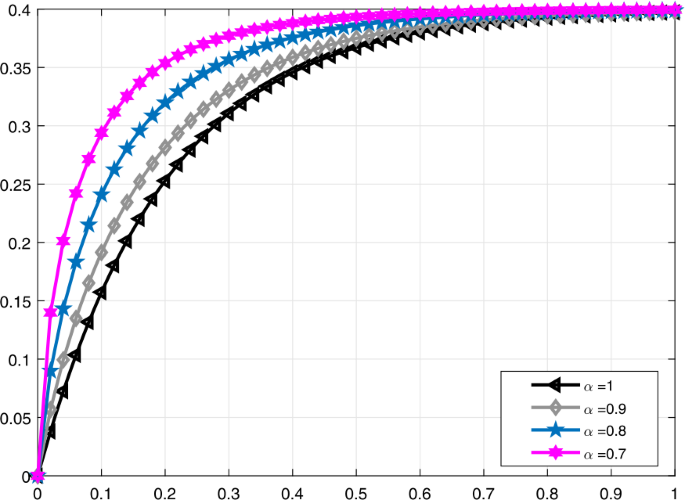
Comparative analysis with truncated M-derivative for \(\mathcal{V}_{i}(t)\), \(\beta =0.8\)
Figure 2 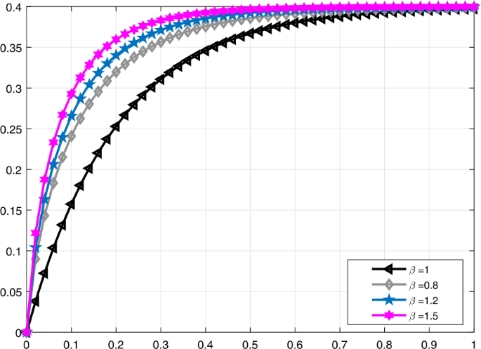
Comparative analysis with truncated M-derivative for \(\mathcal{V}_{i}(t)\), \(\alpha =0.8\)
-
In Fig. 3, a comparison is made for \(\mathcal{V}_{i}(t)\) when \(\alpha =1,0.95,0.82,0.68\), and in Fig. 4, it is made for \(\alpha =1,0.95,0.9,0.85\). Moreover, in Fig. 5 the solution curves of \(\mathcal{V}_{i}(t)\) are shown by means of proportional derivative for \(\alpha =1,0.65,0.45,0.25\) and in Fig. 6 for \(\alpha =1,0.9,0.8,0.7\).
Figure 3 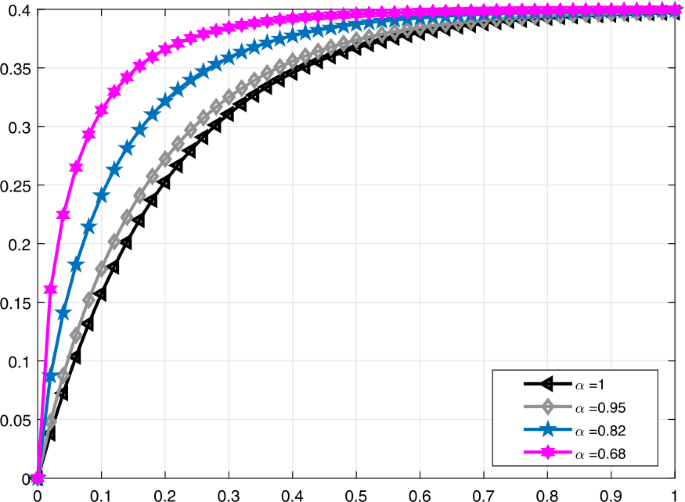
Comparative analysis with conformable derivative for \(\mathcal{V}_{i}(t)\)
Figure 4 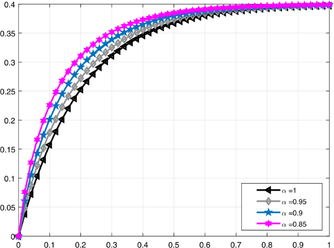
Comparative analysis with conformable derivative for \(\mathcal{V}_{i}(t)\)
Figure 5 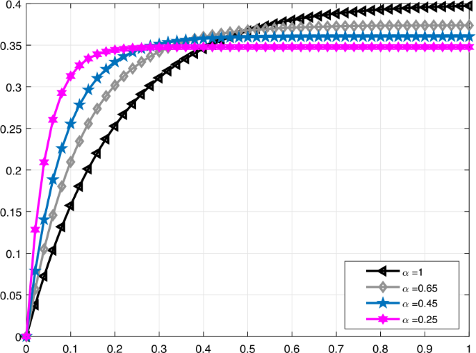
Comparative analysis with proportional derivative for \(\mathcal{V}_{i}(t)\)
Figure 6 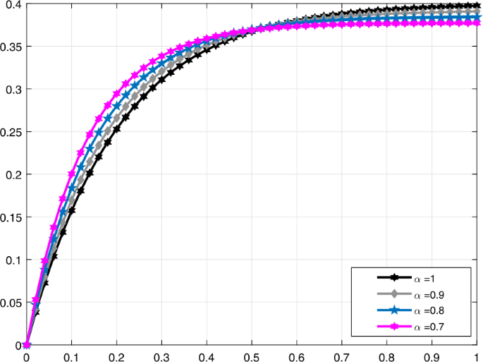
Comparative analysis with proportional derivative for \(\mathcal{V}_{i}(t)\)
-
In Figs. 7 and 8, we compare the proportional derivative, truncated M-derivative, and conformable derivative with the traditional one for the function \(\mathcal{V}_{i}(t)\) when \(\alpha =0.75\), \(\beta =0.5\) and \(\alpha =0.9\), \(\beta =0.8\), respectively. We can clearly seen that the proportional derivative tends to be close to the classical derivative faster than the truncated M-derivative and conformable derivative.
Figure 7 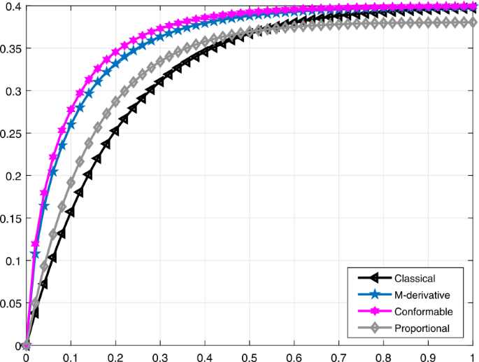
Comparative analysis when \(\alpha =0.75\) and \(\beta =0.5\) for \(\mathcal{V}_{i}(t)\)
Figure 8 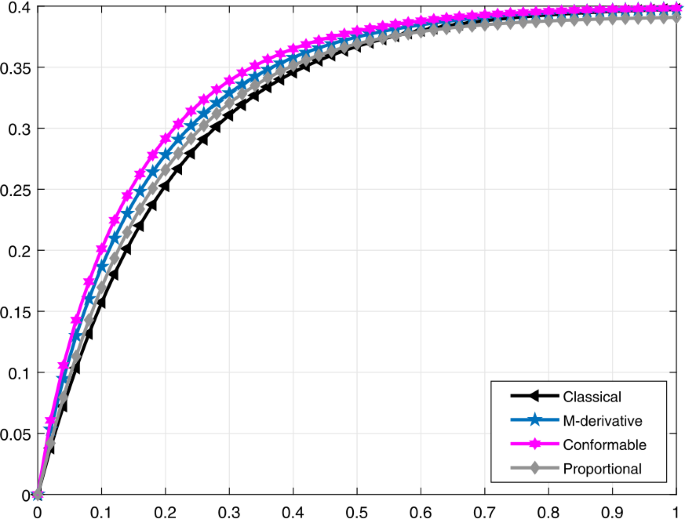
Comparative analysis when \(\alpha =0.9\) and \(\beta =0.8\) for \(\mathcal{V}_{i}(t)\)
-
Lastly, in Figs. 9–12, similar comparisons for the function \(\mathcal{V}_{e}(t)\) are presented, which enables us to observe the decrease in volume of the lung during expiration at different times t for different values of α and β.
Figure 9 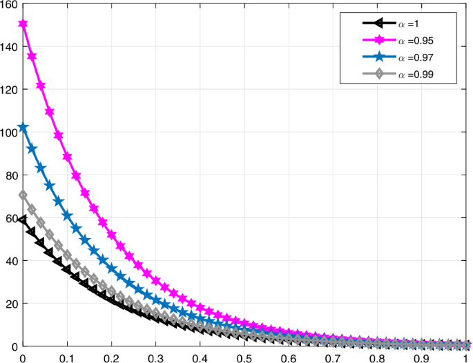
Comparative analysis with proportional derivative for \(\mathcal{V}_{e}(t)\)
Figure 10 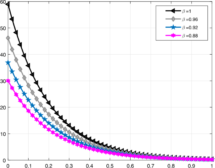
Comparative analysis with truncated M-derivative for \(\mathcal{V}_{e}(t)\), \(\alpha =1\)
Figure 11 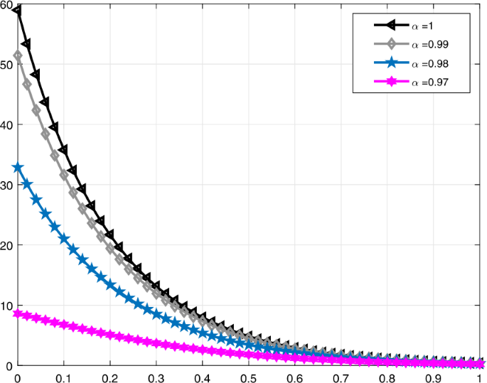
Comparative analysis with conformable derivative for \(\mathcal{V}_{e}(t)\)
Figure 12 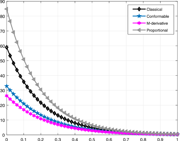
Comparative analysis when \(\alpha =0.98\) and \(\beta =0.96\) for \(\mathcal{V}_{e}(t)\)
-
It should be noted that all graphs are plotted for \(R=10\) cm (H2O)/L/sec, \(C=0.02\text{ L}/\text{cm}\)(H2O), \(P_{d}=20\) cm (H2O), \(t_{j}=1\) sec, and \(t_{b}=3\) sec. Additionally, note that all solutions obtained by the proportional derivative, truncated M-derivative, and conformable derivative correspond to the classical solution of the model analyzed when \(\alpha =1\).


Availability of data and materials
Data sharing not applicable to this paper as no datasets were generated or analyzed during the current study.
References
Nagle, R.K., Saff, E.B., Snider, A.D.: Fundamentals of Differential Equations. Pearson Education, Upper Saddle River (2014)
Kilbas, A.A.A., Srivastava, H.M., Trujillo, J.J.: Theory and Applications of Fractional Differential Equations, vol. 204. Elsevier, Amsterdam (2006)
Caputo, M., Fabrizio, M.: A new definition of fractional derivative without singular kernel. Prog. Fract. Differ. Appl. 1, 1–13 (2015)
Atangana, A., Baleanu, D.: New fractional derivatives with nonlocal and non-singular kernel: theory and application to heat transfer model (2016). arXiv preprint arXiv:1602.03408
Baleanu, D., Fernandez, A.: On fractional operators and their classifications. Mathematics 7, 830 (2019)
Khalil, R., Al Horani, M., Yousef, A., Sababheh, M.: A new definition of fractional derivative. J. Comput. Appl. Math. 264, 65–70 (2014)
Katugampola, U.N.: A new fractional derivative with classical properties (2014). arXiv preprint arXiv:1410.6535
Sousa, J.V.D.C., de Oliveira, E.C.: A new truncated M-fractional derivative type unifying some fractional derivative types with classical properties (2017). arXiv preprint arXiv:1704.08187
Atangana, A., Baleanu, D., Alsaedi, A.: Analysis of time-fractional Hunter–Saxton equation: a model of neumatic liquid crystal. Open Phys. 14, 145–149 (2016)
Abdeljawad, T.: On conformable fractional calculus. J. Comput. Appl. Math. 279, 57–66 (2015)
Abdeljawad, T., Alzabut, J., Jarad, F.: A generalized Lyapunov-type inequality in the frame of conformable derivatives. Adv. Differ. Equ. 2017, 321 (2017)
Yavuz, M.: Novel solution methods for initial boundary value problems of fractional order with conformable differentiation. Int. J. Optim. Control Theor. Appl. 8, 1–7 (2017)
Horani, M.A., Hammad, M.A., Khalil, R.: Variation of parameters for local fractional nonhomogeneous linear differential equations. J. Math. Comput. Sci. 16, 147–153 (2016)
Anderson, D.R.: Second-order self-adjoint differential equations using a conformable proportional derivative (2016). arXiv preprint arXiv:1607.07354
Anderson, D.R., Ulness, D.J.: Newly defined conformable derivatives. Adv. Dyn. Syst. Appl. 10, 109–137 (2015)
Li, Y., Ang, K.H., Chong, G.C.: PID control system analysis and design. IEEE Control Syst. Mag. 26, 32–41 (2006)
Jarad, F., Abdeljawad, T., Alzabut, J.: Generalized fractional derivatives generated by a class of local proportional derivatives. Eur. Phys. J. Spec. Top. 226, 3457–3471 (2017)
Jarad, F., Uğurlu, E., Abdeljawad, T., Baleanu, D.: On a new class of fractional operators. Adv. Differ. Equ. 2017, 247 (2017)
Jarad, F., Abdeljawad, T.: Generalized fractional derivatives and Laplace transform. Discrete Contin. Dyn. Syst., Ser. S 13(3), 709–722 (2019)
Abdeljawad, T., Jarad, F., Alzabut, J.: Fractional proportional differences with memory. Eur. Phys. J. Spec. Top. 226, 3333–3354 (2017)
Morales-Delgado, V.F., Gomez-Aguilar, J.F., Taneco-Hernandez, M.A.: Analytical solutions of electrical circuits described by fractional conformable derivatives in Liouville–Caputo sense. AEÜ, Int. J. Electron. Commun. 85, 108–117 (2018)
Baleanu, D., Fernandez, A., Akgül, A.: On a fractional operator combining proportional and classical differintegrals. Mathematics 8, 360 (2020)
Qureshi, S., Yusuf, A., Shaikh, A.A., Inc, M., Baleanu, D.: Fractional modeling of blood ethanol concentration system with real data application. Chaos, Interdiscip. J. Nonlinear Sci. 29, 013143 (2019)
Yusuf, A., Inc, M., Aliyu, A.I.: On dark optical solitons of the space time nonlinear Schrödinger equation with fractional complex transform for Kerr and power law nonlinearities. J. Coupled Syst. Multiscale Dyn. 6, 114–120 (2018)
Acay, B., Bas, E., Abdeljawad, T.: Fractional economic models based on market equilibrium in the frame of different type kernels. Chaos Solitons Fractals 130, 109438 (2020)
Acay, B., Bas, E., Abdeljawad, T.: Non-local fractional calculus from different viewpoint generated by truncated M-derivative. J. Comput. Appl. Math. 366, 112410 (2020)
Bas, E., Acay, B., Ozarslan, R.: The price adjustment equation with different types of conformable derivatives in market equilibrium. AIMS Math. 4(3), 805–820 (2019)
Acay, B., Ozarslan, R., Bas, E.: Fractional physical models based on falling body problem. AIMS Math. 5, 2608 (2020)
Sajjadi, S.S., Baleanu, D., Jajarmi, A., Pirouz, H.M.: A new adaptive synchronization and hyperchaos control of a biological snap oscillator. Chaos Solitons Fractals 138, 109919 (2020)
Baleanu, D., Jajarmi, A., Sajjadi, S.S., Asad, J.H.: The fractional features of a harmonic oscillator with position-dependent mass. Commun. Theor. Phys. 72, 055002 (2020)
Jajarmi, A., Yusuf, A., Baleanu, D., Inc, M.: A new fractional HRSV model and its optimal control: a non-singular operator approach. Phys. A, Stat. Mech. Appl. 547, 123860 (2020)
Baleanu, D., Jajarmi, A., Mohammadi, H., Rezapour, S.: A new study on the mathematical modelling of human liver with Caputo–Fabrizio fractional derivative. Chaos Solitons Fractals 134, 109705 (2020)
Jajarmi, A., Baleanu, D.: On the fractional optimal control problems with a general derivative operator. Asian J. Control (2019)
Xiao-Jun, Y.A.N.G.: The vector power-law calculus with applications in power-law fluid flow. Therm. Sci. 24, 4289–4302 (2020)
Yang, X.J.: On traveling-wave solutions for the scaling-law telegraph equations. Therm. Sci. 24, 3861–3868 (2020)
Acknowledgements
B. Almohsen is supported by Researchers Supporting Project number (RSP-2020/158), King Saud University, Riyadh, Saudi Arabia.
Funding
The work was supported by Huzhou University (61673169, 11301127, 11701176, 11626101, 11601485).
Author information
Authors and Affiliations
Contributions
All authors read and approved the final manuscript.
Corresponding authors
Ethics declarations
Competing interests
The authors declare that they have no competing interests.
Rights and permissions
Open Access This article is licensed under a Creative Commons Attribution 4.0 International License, which permits use, sharing, adaptation, distribution and reproduction in any medium or format, as long as you give appropriate credit to the original author(s) and the source, provide a link to the Creative Commons licence, and indicate if changes were made. The images or other third party material in this article are included in the article’s Creative Commons licence, unless indicated otherwise in a credit line to the material. If material is not included in the article’s Creative Commons licence and your intended use is not permitted by statutory regulation or exceeds the permitted use, you will need to obtain permission directly from the copyright holder. To view a copy of this licence, visit http://creativecommons.org/licenses/by/4.0/.
About this article

Cite this article
Acay, B., Inc, M., Chu, YM. et al. Modeling of pressure–volume controlled artificial respiration with local derivatives. Adv Differ Equ 2021, 49 (2021). https://doi.org/10.1186/s13662-020-03204-9
Received:
Accepted:
Published:
DOI: https://doi.org/10.1186/s13662-020-03204-9