
Abstract
A numerical approach for solving second order singularly perturbed boundary value problems (SPBVPs) is introduced in this paper. This approach is based on the basis function of a 6-point interpolatory subdivision scheme. The numerical results along with the convergence, comparison and error estimation of the proposed approach are also presented.
1 Introduction
The singularly perturbed boundary value problems (SPBVPs) frequently occur in the different areas of physical phenomena. Specifically, these occur in the fields of fluid dynamic, elasticity, neurobiology, quantum mechanics, oceanography, and reactor diffusion process. These problems often have sharp boundary layers. These boundary layers usually appear as a multiple of the highest derivative. Their small values cause trouble in different numerical schemes for the solution of SPBVPs. Therefore, it is important to find the numerical and analytic solutions of these types of problems. The different second order SPBVPs have different expressions but we deal with the following:
where \(0 < \varepsilon < 1\), while \(p(u)\), \(q(u)\), \(g(u)\) are bounded and real valued functions. \(g(u)\), \(\alpha _{0}\), \(\alpha _{1}\) depends on ε. We may refer to Ascher et al. [1] for more details as regards such a type of SPBVPs.
Here, we first present short review of different methods for the solution of second order SPBVPs; then we discuss a subdivision-based solution of SPBVPs.
The second order SPBVPs were solved based on cubic spline scheme by Aziz and Khan [2, 6] in 2005. These problems were also solved by Bawa and Natesan [3] in the same year. They have used quintic spline based approximating schemes. Kadalbajoo and Aggarwal [5] and Tirmizi et al. [17] solved self-adjoint SPBVPs by using B-spline collocation and non-polynomial spline function schemes, respectively. Kumar and Mehra [7] and Pandit and Kumar [14] solved SPBVPs by a wavelet optimized difference and uniform Haar wavelet methods, respectively.
The second order SPBVPs were also solved by [9, 12, 13]. They have used finite difference scheme for the solution.
The linear SPBVPs were solved by [4, 11, 15]. They have used interpolating subdivision schemes for this purpose. The solution of second order SPBVPs by subdivision techniques did not reported yet. We develop an algorithm by using a 6-point interpolating subdivision scheme (6PISS) [8]. We have
where the scheme is \(C^{2}\)-continuous for \(0<\mu <0.042\). It has support width \((-5, 5)\). It has fourth order of approximation. It satisfies the 2-scale relation
where
Here is the layout of the rest of the work. In Sect. 2, we first find the derivatives of \(\rho (u)\) then by using them we develop the collocation algorithm. The convergence of the method is discussed in Sect. 3. In Sect. 4, we present the numerical solutions of different problems. The comparison of the solutions obtained by different methods is also offered. Section 5 deals with our conclusion.
2 The numerical algorithm
In this section, we develop an algorithm to deal with second order SPBVPs. First we discuss the derivatives of 2-scale relations known as basis functions of the subdivision scheme.
2.1 Derivatives of 2-scale relations
The 6PISS is \(C^{2}\)-continuous by [8], so its 2-scale relations \(\rho (u)\) are also \(C^{2}\)-continuous. First we find the eigenvectors (both left and right) of the subdivision matrix of 6PISS then we find the derivatives of \(\rho (u)\). For simplicity, we choose \(\mu =0.04\) to find eigenvectors. We use a similar approach to [4, 11] to find the derivatives. The first two derivatives of the 2-scale relation are given in Table 1.
2.2 The 6PISS based algorithm
Let m be the indexing parameter which might be equal to or greater than the last right end integral value of the right eigenvector corresponding to the eigenvalue \(\frac{1}{2}\) of the subdivision matrix for (3). Some useful notations depending on the indexing parameter m are defined as \(h=1/m\) and \(\upsilon _{\kappa _{1}}=\kappa _{1}/m=ih\) with \(\kappa _{1}=0,1,2,\ldots,m\). Finally, we suppose that the approximate solution of (1) is
where \(\{d_{\kappa _{1}}\}\) are the unknowns to be determined; then
with given boundary conditions at both ends of the interval
From (6), we have
We get the system of equations by using (6) and (8) in (7),
where \(A_{\kappa }=p(\upsilon _{\kappa })\), \(q_{\kappa }=q(\upsilon _{\kappa })\) and \(g_{\kappa }=g(\upsilon _{\kappa })\). This implies
This further implies
where \(\kappa =0, 1, 2,\ldots, m\) and \(\upsilon _{\kappa _{1}}=ih\) or \(\upsilon _{\kappa }=jh\). By using the notation “\(\rho (\kappa _{1})=\rho _{\kappa _{1}}\)”, (9) can be written as
As we observe from Table 1, \(\rho ^{\bullet }_{-\kappa _{1}}=-\rho ^{\bullet }_{\kappa _{1}}\) and \(\rho ^{\bullet \bullet }_{-\kappa _{1}}=\rho ^{\bullet \bullet }_{ \kappa _{1}}\), for \(\kappa =0, 1, 2,\ldots, m\), (10) becomes
The above system of equations is summarized in the following proposition.
Proposition 1
The equivalent form of the system (11) is
where
Proof
Substituting \(\kappa =0\) in (11), we get
By expanding the above equation, we get
Since the support width of the 6PISS is \((-5,5)\) therefore the graphs of \(\rho ^{\bullet }_{\kappa _{1}}\) and \(\rho ^{\bullet \bullet }_{\kappa _{1}}\) cannot be zero over the domain \([-4, 4]\) but their graphs away from it will be zero. This simplifies as
By substituting the values of \(\rho _{\kappa _{1}}\) and \(\rho ^{\bullet }_{0}=0\), we get
If
the above equation becomes
Similarly, for \(\kappa =1, 2, 3,\ldots, m\), we get
where, for \(\kappa _{1}= -4, -3,\ldots, 3, 4\) and \(\kappa =1, 2, 3,\ldots, m\), we have
The proof has been completed. □
2.2.1 Matrix representation of the linear system
The matrix representation of the linear system (12) is given by
where
where \(r=1, 2,\ldots,m+2\) and \(s=-4, -3,\ldots, m+3, m+4\) represent row and column, respectively, and
The column matrices \(\mathbb{D}\) and \(\mathbb{G}_{1}\) are given by
and
The system (14) in its present form does not have a unique solution. We need eight extra equations to get its unique solution. Luckily, two equations can be obtained from (2), i.e., \(D(0)\) and \(D(1)\) and for the remaining six equations, we move to the next section.
2.2.2 End point constraints
If the data points are given then the 6PISS is suitable to fit the data with a fourth order of approximation. So we use the fourth order polynomials to define the constraints at the end points. Here we suggest two types of polynomials i.e. the simple cubic polynomial (i.e. a polynomial of order 4) and cardinal basis function-based cubic polynomial, to get the constraints.
C-1: Constraints by polynomial of degree three:
We use the fourth order polynomial \(C_{1}(\upsilon )\) which interpolates the data \((\upsilon _{\kappa _{1}}, d_{\kappa _{1}})\) for \(0\leq \kappa _{1} \leq 3\) to compute the left end points \(d_{-3}\), \(d_{-2}\), \(d_{-1}\). Precisely, we have
where
Since by (6), \(D(\upsilon _{\kappa _{1}})=d_{\kappa _{1}}\) for \(\kappa _{1}=1, 2, 3\) then, by replacing \(\upsilon _{\kappa _{1}}\) by \(-\upsilon _{\kappa _{1}}\), we have
Hence, we get the following three constraints defined at the left end points:
A similar procedure is adopted for the right end i.e. we can define \(d_{\kappa _{1}}=C_{1}(\upsilon _{\kappa _{1}})\), \(\kappa _{1}= m+1, m+2, m+3\) and
So the following three constraints are defined at the right end:
C-2: Constraints by cardinal basis functions:
The following fourth order polynomial \(C_{2}(\upsilon )\) can be used to find the left points \(d_{-3}\), \(d_{-2}\), \(d_{-1}\):
where
while the basis functions are given by
and for \(t=0, 1\)
A similar procedure is adopted for the right end points \(d_{\kappa _{1}}=C_{2}(-\upsilon _{\kappa _{1}})\), \(\kappa _{1}= m+1, m+2, m+3\), where
and
and for \(t=m, m+1\)
2.2.3 Stable singularly perturbed system
Finally, we get a stable singularly perturbed system with \(m+9\) unknowns and \(m+9\) equations obtained from (2), (12), (18) and (19) or (20) and (21).
By C-1 constrants:
If we use (2), (12), (18) and (19) then the system can expressed as
where \(\mathbb{S}_{1}= (\mathbb{S}_{L_{1}}^{T}, \mathbb{S}^{T}, \mathbb{S}_{R_{1}}^{T})^{T}\), \(\mathbb{S}\) is defined by (15). The matrix \([\mathbb{S}_{L_{1}}]_{4\times (m+9)}\) is defined as
its first three rows and the fourth row are obtained from (18) and (2), respectively,
its first row and the last three rows are obtained from (2) and (19), respectively,
while the matrices \(\mathbb{D}\) and \(\mathbb{G}_{1}\) are defined in (16) and (17), respectively.
By C-2 constraints:
If we use (2), (12), (20) and (21) then the system can be expressed as
where \(\mathbb{S}_{2}= (\mathbb{S}_{L_{2}}^{T}, \mathbb{S}^{T}, \mathbb{S}_{R_{2}}^{T})^{T}\) while the first three rows and the last row of \([{\mathbb{S}_{L_{2}}}]_{4\times (m+9)}\) are obtained from (20) and (2), respectively. Similarly the first row and the remaining three rows of \([{\mathbb{S}_{R_{2}}}]_{4\times (m+9)}\) are obtained from (2) and (21), respectively. Now we have two systems, i.e., (22) and (24).
2.3 Existence of the solution
The matrices \(\mathbb{S}_{1}\) and \(\mathbb{S}_{2}\) involved in the systems (22) and (24) are non-singular. Their non-singularity can be checked by finding their eigenvalues. We notice that for \(m\leq 500\) the eigenvalues are nonzero. By [16], these are non-singular. Their singularity is not guaranteed for \(m > 500\).
3 Error estimation of the algorithm
This section discussed the mathematical results as regards the convergence of the proposed method.
Let the analytic solution of the SPBVPs problem (1) with (2) be denoted as \(Z_{e}\) then
It implies for node points, \(\kappa =0, 1,\ldots,m\),
Let the vector \(Z_{e}(\upsilon )\) be defined as
By Taylor’s series
and
Since \(D(\upsilon )\) is the approximate solution of (1) which can be obtained from the system (22) or (24), by (7), for \(\kappa =0, 1,\ldots, m\), we have
where \(D^{\bullet }(\upsilon _{\kappa })\) and \(D^{\bullet \bullet }(\upsilon _{\kappa })\) are defined as
and
Let the error function \(\Delta (\upsilon )=Z_{e}(\upsilon )-D(\upsilon )\) and
Then error vector at the given nodal values is
This implies
The following result is obtained after subtracting (26) from (25):
By applying the definition of error vector the above equation can be written as
This implies
where for \(0\leqslant \kappa \leqslant m\)
and for \(0\leqslant \kappa \leqslant m\)
As \(0\leq \upsilon \leq 1\) and \(\upsilon _{\kappa }=\kappa h\), \(\kappa =0,1, 2,\ldots, m\), the values lie outside the interval \([0,1]\), i.e., \(\Delta _{-4},\ldots, \Delta _{-1}\) and \(\Delta _{m+1},\ldots, \Delta _{m+4}\) must be equal to zero. These error values can be assumed to be
If we expand (27) by adopting a similar procedure to Proposition 1 then we obtain
and
Or equivalently
and
The matrix \(\mathbb{S}_{\kappa _{1}}+\mathcal{O}(h^{4})\), \(\kappa _{1}=1, 2\), for small h and \(\epsilon =0.1 \times 10^{-3}\), is non-singular so
Hence \(\Vert \Delta \Vert = O(h^{4})\). This discussion can be summarized.
Proposition 2
Let\(Z_{e}\)and\(D_{\kappa }\), \(\kappa =0,1,\ldots, m \)be the analytic and approximate solutions of second order SPBVPs defined in (1), respectively, then\(\Vert \Delta \Vert = \Vert Z_{e}(\upsilon )-D(\upsilon ) \Vert \leq \mathcal{O}(h^{4})\).
Remark
The order of error approximation varies if we use different values of ϵ.
4 Solutions of second order SPBVPs and discussions
In this section, we consider second order SPBVPs and find their numerical solutions by using different algorithms. Since we have developed two linear systems i.e. (22) and (24) for approximate solutions of the SPBVPs, both systems have been used for solutions. We also give a comparison of solutions by computing the maximum absolute errors of the analytic and approximate solutions.
Example 4.1
This type of problem has also solved by [2, 3, 5, 6, 14],
where the boundary conditions of the above problem are
its analytic solution is
Example 4.2
Consider the boundary value problem [10, 12, 13]
where the boundary conditions of the above problem are
its analytic solution is
Example 4.3
Take the problem already solved by [7, 9],
here \(0\leqslant \upsilon \leqslant 1\) and
its analytic solution is
4.1 Discussion and comparison
We solve SPBVPs by our algorithm and summarized the results in the following form.
The facts regarding the solutions of Example 4.1 are shown in Tables 2–6 and in Figs. 1–3 In Tables 2 and 3, the maximum absolute errors (MAE) are given while in Tables 4–6 the comparison with the methods of [2, 3, 5, 6, 14] are presented. In Fig. 1 the solutions are presented. In Figs. 2 and 3 results for m and ε are depicted.
Figure 1 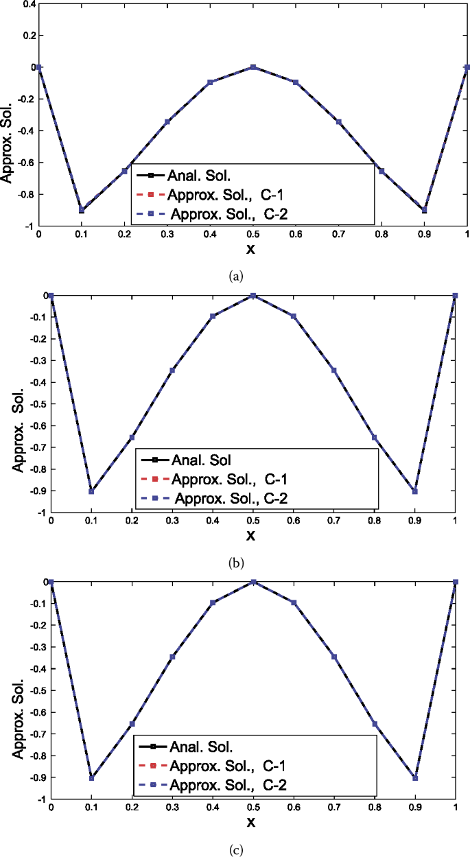
Comparison concerning Example 4.1: Analytic and approximate solutions with parametric setting: \(N=10\) and \(\varepsilon =10^{-4}, 10^{-7}, 10^{-10}\)
Figure 2 
Comparison concerning Example 4.1: Analytic and approximate solutions with parametric setting: \(N=32\) and \(\varepsilon =2^{-25}\)
Figure 3 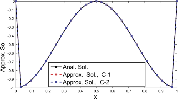
Comparison concerning Example 4.1: Analytic and approximate solutions with parametric setting: \(N=32\) and \(\varepsilon =(2^{-20})^{2}\)
Table 2 Maximum absolute errors (MAE) for Example 4.1 Table 3 MAE in the solution of SPBVP in Example 4.1 Table 4 MAE in the solution of SPBVP in Example 4.1 Table 5 MAE in the solution of SPBVP in Example 4.1 Table 6 MAE in the solution of SPBVP in Example 4.1 In Tables 7–10 and in Figs. 4–6 results of Example 4.2 are presented. Tables 7 and 10 show the MAE while Tables 9 and 10 present the comparison of MAE with [10, 12, 13]. This shows our results are better. Figure 4 shows the solutions while Figs. 5 and 6 show the results for m and ε.
Figure 4 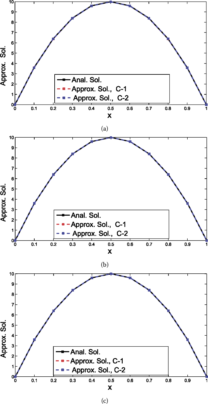
Comparison concerning Example 4.2: Analytic and approximate solutions with parametric setting: \(N=10\) with \(\varepsilon =10^{-4}, 10^{-7}, 10^{-10}\)
Figure 5 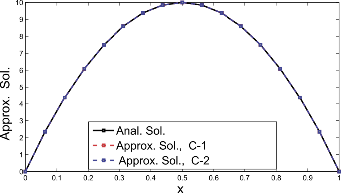
Comparison concerning Example 4.2: Analytic and approximate solutions with parametric setting: \(N=16\) and \(\varepsilon =10^{-8}\)
Figure 6 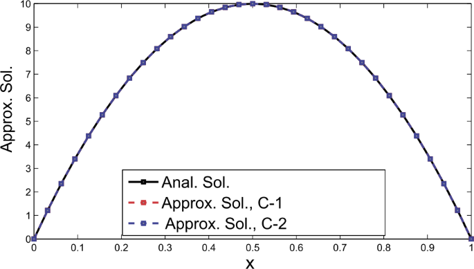
Comparison concerning Example 4.2: Analytic and approximate solutions with parametric setting: \(N=32\) and \(\varepsilon =10^{-9}\)
Table 7 MAE in the solution of SPBVP in Example 4.2 Table 8 MAE in the solution of SPBVP in Example 4.2 Table 9 MAE in the solution of SPBVP in Example 4.2 Table 10 MAE in the solution of SPBVP in Example 4.2 Tables 11–13 and Figs. 7–9 are related to the solution of Example 4.3. The MAE are shown in Tables 11 and 12. We compare our result with the results of [7, 9] and found them to be better. The graphical representation is given in Figs. 8 and 9
Figure 7 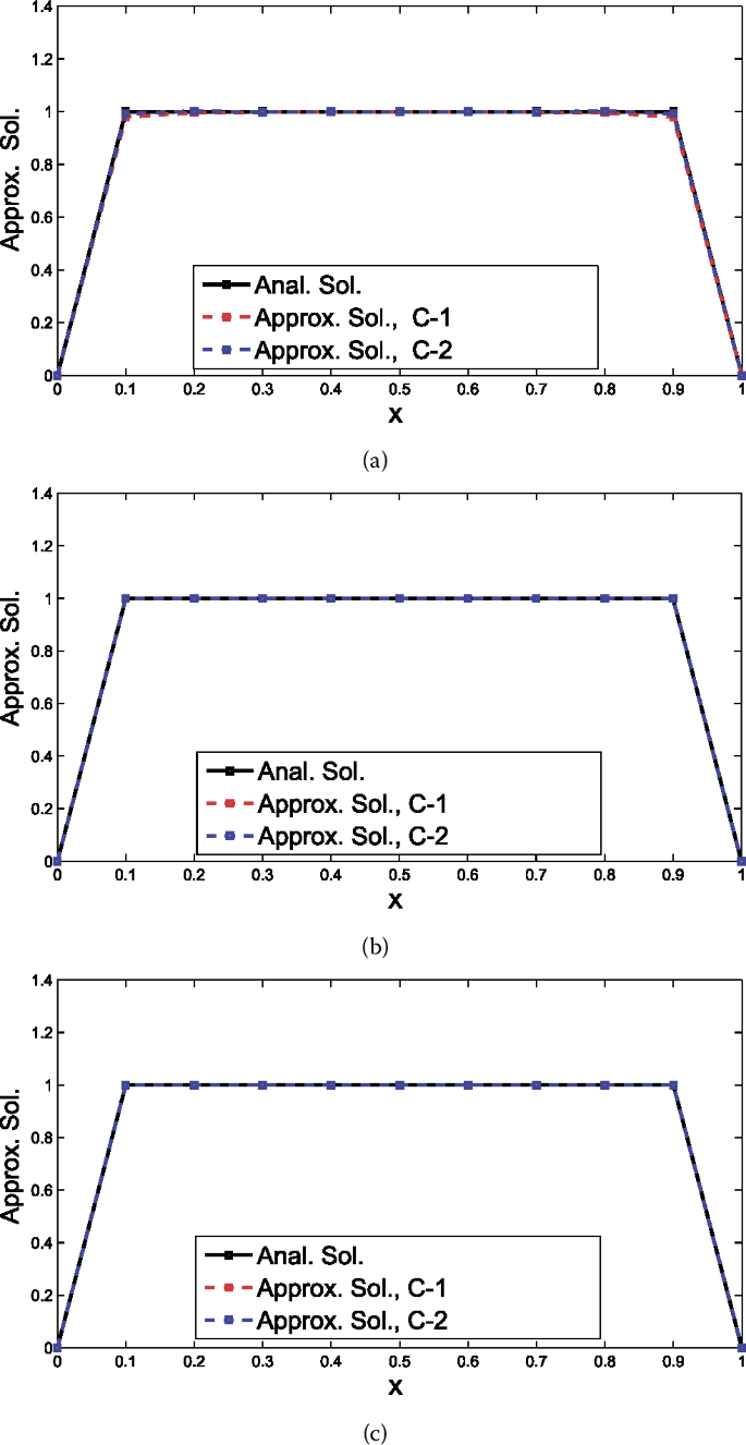
Comparison concerning Example 4.3: Analytic and approximate solutions with parametric setting: \(N=10\) with \(\varepsilon =10^{-4}, 10^{-7}, 10^{-10}\) shown in (a), (b) and (c), respectively
Figure 8 
Comparison concerning Example 4.3: Analytic and approximate solutions with parametric setting: \(N=16\) and \(\varepsilon =10^{-5}\)
Figure 9 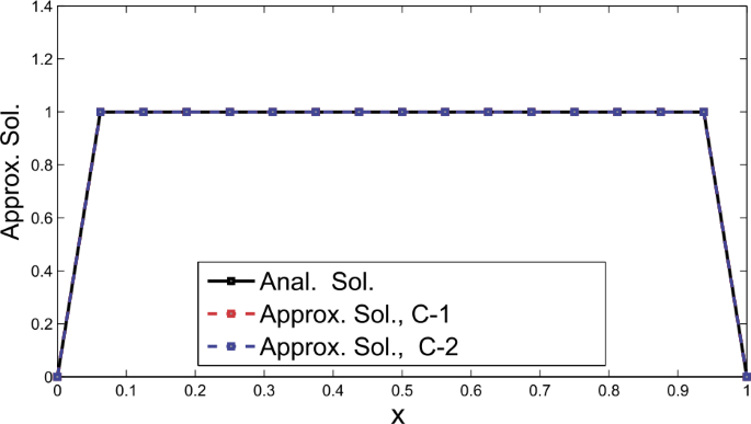
Comparison concerning Example 4.3: Analytic and approximate solutions with parametric setting: \(N=16\) and \(a=10^{-8}\)
Table 11 MAE in the solution of SPBVP in Example 4.3 Table 12 MAE in the solution of SPBVP in Example 4.3 Table 13 MAE in the solution of SPBVP in Example 4.3 From these results we conclude that the condition C-2 gives better results than the condition C-1.
If we keep m fixed, then MAE increases with the increase of ε. It is also observed that if we keep ε fixed, then MAE decreases with the increase of m.


5 Conclusions
In this paper, we introduced a numerical algorithm for the solution of second order SPBVPs. The algorithm was developed by using the 2-scale relation of a well-known interpolating subdivision scheme. This algorithm gives the approximate solution of second order SPBVPs with a fourth order of approximation. We presented the comparison of maximum absolute error of the solutions obtained from subdivision (i.e. our method), spline [2, 3, 5, 6], finite difference [9, 10, 12, 13] and Haar wavelet [7, 14] algorithms. We concluded that our algorithm gives smaller maximum absolute error.
References
Ascher, U.M., Mattheij, R.M.M., Russell, R.D.: Numerical Solution of Boundary Value Problems for Ordinary Differential Equations. Prentice Hall, Englewood Cliffs (1988)
Aziz, T., Khan, A.: A spline method for second order singularly perturbed boundary value problems. J. Comput. Appl. Math. 147, 445–452 (2002)
Bawa, R.K., Natesan, S.: A computational method for self adjoint singular perturbation problem using quintic spline. Comput. Math. Appl. 50, 1371–1382 (2005)
Ejaz, S.T., Mustafa, G., Khan, F.: Subdivision schemes based collocation algorithms for solution of fourth order boundary value problems. Math. Probl. Eng. 2015, Article ID 240138 (2015)
Kadalbajoo, M.K., Aggarwal, V.K.: Fitted mesh B-spline collocation method for solving self-adjoint singularly perturbed boundary value problems. Appl. Math. Comput. 161, 973–987 (2005)
Khan, I., Aziz, T.: Tension spline method for second order singularly perturbed boundary value problems. Int. J. Comput. Math. 82(12), 1547–1553 (2005)
Kumar, V., Mehra, M.: Wavelet optimized finite difference method using interpolating wavelets for self-adjoint singularly perturbed problems. J. Comput. Appl. Math. 230(2), 803–812 (2009)
Lee, B.G., Lee, Y.J., Yoon, J.: Stationary binary subdivision schemes using radial basis function interpolation. Adv. Comput. Math. 25, 57–72 (2006)
Lubuma, J.M.S., Patidar, K.C.: Uniformly convergent non-standard finite difference methods for self-adjoint singularly perturbed problems. J. Comput. Appl. Math. 191, 228–238 (2006)
Miller, J.J.H.: On the convergence, uniformly in ε, of difference schemes for a two point singular perturbation problem. In: Numerical Analysis of Singular Perturbation Problems, pp. 467–474. Academic Press, New York (1979)
Mustafa, G., Ejaz, S.T.: Numerical solution of two point boundary value problems by interpolating subdivision schemes. Abstr. Appl. Anal. 2014, Article ID 721314 (2014)
Niijima, K.: On a finite difference scheme for a singular perturbation problem without a first derivative term I. Mem. Numer. Math. 7, 1–10 (1980)
Niijima, K.: On a finite difference scheme for a singular perturbation problem without a first derivative term II. Mem. Numer. Math. 7, 11–27 (1980)
Pandit, S., Kumar, M.: Haar wavelet approach for numerical solution of two parameters singularly perturbed boundary value problems. Appl. Math. Inf. Sci. 8(6), 2965–2974 (2014)
Qu, R., Agarwal, R.P.: Solving two point boundary value problems by interpolatory subdivision algorithms. Int. J. Comput. Math. 60, 279–294 (1996)
Strang, G.: Linear Algebra and Its Applications. Cengage Learning India Private Limited (2011). ISBN 81-315-0172-8
Tirmizi, I.A., i-Haq, F., ul-Islam, S.: Non-polynomial spline solution of singularly perturbed boundary value problems. Appl. Math. Comput. 196, 6–16 (2008)
Acknowledgements
This work is supported by Indigenous Ph.D. Scholarship Scheme of HEC Pakistan. The first author is supported by HEC, NRPU (P. No. 3183) and second author is grateful to Higher Education Commission Pakistan for granting scholarship for Ph. D studies.
Availability of data and materials
“Data sharing not applicable to this article as no datasets were generated or analysed during the current study.”
Funding
“Not available.”
Author information
Authors and Affiliations
Contributions
The authors have contributed equally to this manuscript. They read and approved the final manuscript.
Corresponding author
Ethics declarations
Competing interests
The authors declare that they have no competing interests.
Rights and permissions
Open Access This article is licensed under a Creative Commons Attribution 4.0 International License, which permits use, sharing, adaptation, distribution and reproduction in any medium or format, as long as you give appropriate credit to the original author(s) and the source, provide a link to the Creative Commons licence, and indicate if changes were made. The images or other third party material in this article are included in the article’s Creative Commons licence, unless indicated otherwise in a credit line to the material. If material is not included in the article’s Creative Commons licence and your intended use is not permitted by statutory regulation or exceeds the permitted use, you will need to obtain permission directly from the copyright holder. To view a copy of this licence, visit http://creativecommons.org/licenses/by/4.0/.
About this article

Cite this article
Mustafa, G., Ejaz, S.T., Baleanu, D. et al. A subdivision-based approach for singularly perturbed boundary value problem. Adv Differ Equ 2020, 282 (2020). https://doi.org/10.1186/s13662-020-02732-8
Received:
Accepted:
Published:
DOI: https://doi.org/10.1186/s13662-020-02732-8