
Abstract
In this paper, we consider a model of plant virus propagation with two delays and Holling type II functional response. The stability of the positive equilibrium and the existence of Hopf bifurcation are analyzed by choosing \(\tau_{1}\) and \(\tau_{2}\) as bifurcation parameters, respectively. Using the center manifold theory and normal form method, we discuss conditions for determining the stability and the bifurcation direction of the bifurcating periodic solution. Finally, we carry out numerical simulations to illustrate the theoretical analysis.
1 Introduction
As we know, plants play a vital role in the everyday life of all organisms on earth. Sometimes, however, plants become infected with a virus, which can have a devastating effect on the ecosystem that depends on it. An insect-vector can cause the transmission of the virus from plant to plant. The propagation characteristics and epidemiology of plant viruses were studied in [1, 2]. In [3], the transmission pathways of plant viruses were analyzed in detail from the perspective of plants and media; the authors established a model of plant infections disease and analyzed the dynamics of the model.
Although there are many models that describe the interaction between vectors and humans, there are not as many that describe the relationship between plants and vectors. Recently, Jackson and Chen-Charpentier [4] have proposed a plant virus propagation model with the functional response Holling type II of the following form:
where \(S(t), I(t), R(t), X(t)\), and \(Y(t)\) denote the susceptible plants, infected plants, recovered plants, susceptible insect vectors, and infected insect vectors, respectively. The total number of plants will be denoted by the fixed positive constant \(K, K=S+I+R\), and the total number of insects will be denoted by \(N=X+Y\). The parameters \(\beta, \beta_{1}, \alpha, \alpha_{1}, \mu, m, \gamma, \Lambda\), and d are positive real numbers; β is the infection rate of plants due to vectors, \(\beta_{1}\) is the infection rate of vectors due to plants, α is the saturation constant of plants due to vectors, \(\alpha_{1}\) is the saturation constant of vectors due to plants, μ is the natural death rate of plants, m is the natural death rate of vectors, γ is the recovery rate of plants, Λ is the replenishing rate of vectors (birth and/or immigration), and d is the death rate of infected plants due to the disease.
In the model (1.1) the authors make the following assumptions [4]:
(1) The susceptible plants can be infected only by the infected insect vectors. This model does not consider that infection can be transmitted from plant to plant. The interaction between the insects and the plants is modeled using Holing type II since insects can only bite a limited number of plants.
(2) The total number of plants is denoted by the fixed positive constant K, because in one area, one can always keep the total number fixed by adding a new plant when a plant has died. The new plant shares the same characteristics of the plant it replaced before it was infected.
(3) The replenishment rate of insect vectors is a positive constant Λ, and all of the new born vectors are susceptible.
(4) A susceptible vector can be infected only by an infected plant host, and after it is infected, it will hold the virus for the rest of its life. Further, there is no vertical transmission of the virus, and vectors cannot transmit the virus to another vector.
Notice that adding \(\frac{dX}{dt}\) and \(\frac{dY}{dt}\) yields \(\frac{dN}{dt}=\Lambda-mN\), where \(N=X+Y\), and \(N\longrightarrow\frac{\Lambda}{m}\) as \(t\longrightarrow\infty\).
So equation (1.1) can be reduced to the following equations:
where \(\omega=d+\mu+\gamma\).
In [4], the authors analyzed the stability of equilibria with the basic reproduction number using the generation matrix approach. Considering time for the virus to enter the plant cells and to spread in the plant and time for the virus to infect the insect, the authors proposed the model with two discrete delays:
where \(\tau_{1}\) is the time it takes a plant to become infected after contagion, and \(\tau_{2}\) is the time it takes a vector to become infected after contagion.
Since the delay differential equations are extensively used in the practical life, it is very important to study the stability of differential equations with delays. Recently, a great deal of scholars have achieved very good research results in terms of multidelay differential equations [5–15].
In our paper, we continue the work of Jackson and Chen-Charpentier [4]. Viewing delays as bifurcation parameters, we discuss the stability of equilibrium and the existence of Hopf bifurcation of system (1.3) in four cases: (1) \(\tau_{1}=0, \tau_{2}=0\); (2) \(\tau _{1}>0, \tau_{2}=0\); (3) \(\tau_{1}=\tau_{2}=\tau>0\); (4) \(\tau _{1}\in(0,\tau_{10}), \tau_{2}>0, \tau_{1}\neq\tau_{2}\). When \(\tau_{1}\neq\tau_{2}\), we study the properties of Hopf bifurcation by using the normal form theory and center manifold theorem.
This paper is organized as follows. In Sect. 2, we study the stability of positive equilibrium and the existence of local Hopf bifurcation of system (1.3). In Sect. 3, the direction and stability of Hopf bifurcation are determined by using normal form theory and central manifold theorem. Some numerical simulations are carried out to support our results in Sect. 4. Finally, a conclusion is given in Sect. 5.
2 Stability and existence of Hopf bifurcation
System (1.3) has a unique positive equilibrium \(E(S^{\ast}, I^{\ast}, Y^{\ast})\), provided that the following conditions are satisfied:
- \((H_{1})\) :
-
\(m\omega+K\mu(\beta_{1}+\alpha_{1}m)>dm\), \(\alpha\beta _{1}K\Lambda\mu+m(m\omega+K\mu(\beta_{1}+\alpha_{1}m)-dm)>0\), \(\beta_{1}\beta K\Lambda\mu>m^{2}\mu\omega\), \(\alpha m\mu\omega +\beta(m\omega+K\mu(\beta_{1}+\alpha_{1}m)-dm)>0\),
where
The linearized system of system (1.3) at \(E(S^{\ast}, I^{\ast}, Y^{\ast})\) is
where \(A_{0}=\frac{\beta Y^{\ast}}{1+\alpha Y^{\ast}}\), \(B_{0}=\frac {\beta S^{\ast}}{(1+\alpha Y^{\ast})^{2}}\), \(C_{0}=\frac{\beta _{1}}{(1+\alpha_{1}I^{\ast})^{2}}(\frac{\Lambda}{m}-Y^{\ast})\), and \(D_{0}=\frac{-\beta_{1}I^{\ast}}{1+\alpha_{1}I^{\ast}}\).
The characteristic equation of system (2.1) is
where
Next, we consider the following four cases.
Case \((1)\): \(\tau_{1}=0, \tau_{2}=0\).
The characteristic equation (2.2) becomes
Let
- \((H_{2})\) :
-
\(A_{1}+B_{1}+C_{1}>0\), \(A_{3}+B_{3}+C_{3}+D_{2}>0\), \((A_{1}+B_{1}+C_{1})(A_{2}+B_{2}+C_{2}+D_{1})-(A_{3}+B_{3}+C_{3}+D_{2})>0\).
According to the Routh–Hurwitz criteria, if conditions \((H_{1})\) and \((H_{2})\) hold, then all the roots of (2.3) must have negative real parts. We have the following results.
Theorem 2.1
Assume that \((H_{1})\) and \((H_{2})\) hold. If \(\tau _{1}=\tau_{2}=0\), then the positive equilibrium \(E(S^{\ast},I^{\ast },Y^{\ast})\) of system (1.3) is locally asymptotically stable.
Case \((2)\): \(\tau_{1}>0, \tau_{2}=0\).
The characteristic equation (2.2) reduces to
Let \(\lambda=i\omega_{1}\ (\omega_{1}>0)\) be the root of equation (2.4). Then we have:
It follows that
where
Let \(r_{1}=\omega^{2}_{1}\). Then equation (2.6) becomes
Denote
Thus
If \(E_{23}=(A_{3}+C_{3})^{2}-(B_{3}+D_{2})^{2}<0\), then \(h_{1}(0)<0\) and \(\lim_{r_{1}\longrightarrow+\infty}h_{1}(r_{1})=+\infty\). Equation (2.7) has at least one positive root.
If \(E_{23}=(A_{3}+C_{3})^{2}-(B_{3}+D_{2})^{2}\geq0\) and \(\bigtriangleup_{1}=E^{2}_{21}-3E_{22}\leq0\), then equation (2.7) has no positive root for \(r_{1}\in[0,+\infty)\).
If \(E_{23}=(A_{3}+C_{3})^{2}-(B_{3}+D_{2})^{2}\geq0\) and \(\bigtriangleup_{1}=E^{2}_{21}-3E_{22}>0\), then the equation
has two real roots, \(r^{\ast}_{11}=\frac{-E_{21}+\sqrt {\bigtriangleup_{1}}}{3}\) and \(r^{\ast}_{12}=\frac{-E_{21}-\sqrt {\bigtriangleup_{1}}}{3}\). Because \(h^{\prime\prime}_{1}(r^{\ast}_{11})=2\sqrt {\bigtriangleup_{1}}>0\) and \(h^{\prime\prime}_{1}(r^{\ast}_{12})=-2\sqrt {\bigtriangleup_{1}}<0\), equation (2.7) has at least one positive root if and only if \(r^{\ast}_{11}=\frac{-E_{21}+\sqrt {\bigtriangleup_{1}}}{3}>0\) and \(h_{1}(r^{\ast}_{11})\leq0\), where \(r^{\ast}_{11}\) and \(r^{\ast}_{12}\) are the local minimum and maximum of \(h_{1}(r_{1})\), respectively.
Without loss of generality, we assume that (2.7) has three positive roots, defined by \(r_{11}, r_{12}\), and \(r_{13}\), respectively. Then (2.6) has three positive roots \(\omega_{1k}=\sqrt{r_{1k}},k=1,2,3\). From (2.5) we get
and
where \(k=1,2,3,j=0,1,2,\dots\).
Denote
Next, we verify the transversality condition. Let \(\lambda(\tau_{1})=\alpha_{1}(\tau_{1})+i\omega_{1}(\tau _{1})\) be the root of equation (2.4) near \(\tau_{1}=\tau ^{(j)}_{1k}\) satisfying
Substituting \(\lambda(\tau_{1})\) into (2.4) and taking the derivative with respect to \(\tau_{1}\), we have
By (2.9) we have
where \(\Lambda_{1}=(B_{2}+D_{1})^{2}\omega ^{4}_{1k}+[(B_{3}+D_{2})\omega_{1k}-B_{1}\omega^{3}_{1k}]^{2}>0\). Notice that \(\Lambda_{1}>0, r_{1k}>0\),
and thus \(\frac{d(\operatorname{Re}\lambda({\tau^{(j)}_{1k}}))}{d\tau_{1}}\) has the same sign as \(h'_{1}(r_{1k})\).
To investigate the root distribution of the transcendental equation (2.4), we introduce the result of Ruan and Wei [16].
Lemma 2.1
Consider the exponential polynomial
where \(\tau_{i}\geq0\) \((i=1,2,\ldots,m)\) and \(p_{j}^{(i)}\) \((i=0,1,\ldots, m;j=1,2,\ldots,n)\) are constants. As \((\tau_{1},\tau _{2},\ldots,\tau_{m})\) vary, the sum of the order of the zeros of \(P(\lambda,e^{-\lambda\tau _{1}},\ldots,e^{-\lambda\tau_{m}})\) on the open right half-plane can change only if a zero appears on or crosses the imaginary axis.
According to this analysis, we have the following results.
Theorem 2.2
For \(\tau_{1}>0\) and \(\tau_{2}=0\), suppose that \((H_{1})\) and \((H_{2})\) hold. Then:
-
(i)
If \(E_{23}\geq0\) and \(\bigtriangleup _{1}=E^{2}_{21}-3E_{22}\leq0\), then all roots of equation (2.4) have negative real parts for all \(\tau_{1}\geq0\), and the positive equilibrium \(E(S^{\ast},I^{\ast},Y^{\ast})\) is locally asymptotically stable for all \(\tau_{1}\geq0\).
-
(ii)
If either \(E_{23}<0\) or \(E_{23}\geq0\), \(\bigtriangleup_{1}=E^{2}_{21}-3E_{22}>0\), \(r^{\ast}_{11}>0\), and \(h_{1}(r^{\ast}_{11})\leq0\), then \(h_{1}(r_{1})\) has at least one positive root, and all roots of equation (2.4) have negative real parts for \(\tau_{1}\in[0,\tau_{10})\), and the positive equilibrium \(E(S^{\ast},I^{\ast},Y^{\ast})\) is locally asymptotically stable for all \(\tau_{1}\in[0,\tau_{10})\).
-
(iii)
If (ii) holds and \(h^{\prime}_{1}(r_{1k})\neq0\), then system (1.3) undergoes Hopf bifurcations at the positive equilibrium \(E(S^{\ast},I^{\ast},Y^{\ast })\) for \(\tau_{1}=\tau^{(j)}_{1k}\) \((k=1,2,3;j=0,1,2,\dots)\).
When \(\tau_{1}=0\) and \(\tau_{2}>0\), the stability of the equilibrium \(E(S^{\ast},I^{\ast},Y^{\ast})\) and the existence of Hopf bifurcation can be obtained based on a similar discussion, which we omit in this paper.
Case \((3)\): \(\tau_{1}=\tau_{2}=\tau>0\).
When \(\tau_{1}=\tau_{2}=\tau>0\), the characteristic equation (2.2) becomes
where
Both sides of equation (2.10) are multiple \(e^{\lambda\tau}\), and we obviously get
Let \(\lambda=i\omega_{3}\ (\omega_{3}>0)\) be the root of equation (2.11). Separating the real and imaginary parts, we obtain:
from which it follows that
where
Since \(\sin^{2}\omega_{3}\tau+\cos^{2}\omega_{3}\tau=1\), we have
where
Letting \(r_{3}=\omega^{2}_{3}\), equation (2.14) is transformed into
If all the parameters of system (1.3) are given, then it is easy to get the roots of equation (2.15) by using the Matlab software package. To give the main results in this paper, we make the following assumption.
- \((H_{3})\) :
-
equation (2.15) has at least one positive real root.
Suppose that condition \((H_{3})\) holds. Without loss of generality, we assume that (2.14) has six positive real roots, say \(r_{31}, r_{32}, \ldots, r_{36}\). Then (2.13) has six positive real roots
Thus, if we denote
for \(k=1,2,\ldots,6,j=0,1,2,\ldots \) , then \(\pm i\omega_{3k}\) is a pair of purely imaginary roots of (2.11) corresponding to \(\tau ^{(j)}_{3k}\). Define
Let \(\lambda(\tau)=\alpha_{3}(\tau)+i\omega_{3}(\tau)\) be the root of equation (2.11) near \(\tau=\tau^{(j)}_{3k}\) satisfying
Substituting \(\lambda(\tau)\) into (2.11) and taking the derivative with respect to τ, we have
Letting \(\lambda=\pm i\omega_{3k}\) at the roots of equation (2.11) at \(\tau=\tau^{(j)}_{3k}\), we should compute \(\frac{d\operatorname{Re}(\lambda ((\tau^{(j)}_{3k}))}{d\tau}\). By calculation we get
where
So, we have
Obviously, if condition
- \((H_{4})\) :
-
\(P_{31}P_{33}+P_{32}P_{34}\neq0\)
holds, then \(\frac{d\operatorname{Re}\lambda(\tau)}{d\tau}|_{\lambda=i\omega _{3k}}=\operatorname{Re}[\frac{d\lambda(\tau)}{d\tau}]^{-1}_{\lambda=i\omega _{3k}}\neq0\). Thus, we have the following results.
Theorem 2.3
For system (1.3) with \(\tau_{1}=\tau_{2}=\tau>0\), let \((H_{1})\)–\((H_{4})\) hold. The equilibrium point \(E(S^{\ast },I^{\ast},Y^{\ast})\) is asymptotically stable for \(\tau\in[0,\tau ^{(j)}_{3k})\) and unstable for \(\tau>\tau^{(j)}_{3k}\); Hopf bifurcation occurs when \(\tau=\tau^{(j)}_{3k}\).
Case \((4)\): \(\tau_{1}\in(0,\tau_{10})\), \(\tau_{2}>0\), \(\tau _{1}\neq\tau_{2}\).
We consider (2.2) with \(\tau_{1}\) in its stable interval \([0,\tau _{10})\) and \(\tau_{2}\) considered as a parameter. Let \(\lambda=i\omega^{\ast}_{2}(\omega^{\ast}_{2}>0)\) be a root of equation (2.2). Separating real and imaginary parts leads to
From equation (2.18) we can obtain
where
From equation (2.18) we obtain:
where
Denote \(F_{1}(\omega^{\ast}_{2})={\omega^{\ast }_{2}}^{6}+E_{41}{\omega^{\ast}_{2}}^{4}+E_{42}{\omega^{\ast }_{2}}^{2}+E_{43}+E_{44}\sin(\omega^{\ast}_{2}\tau_{1})+E_{45}\cos (\omega^{\ast}_{2}\tau_{1})\). If \(E_{43}=B^{2}_{3}-D^{2}_{2}-C^{2}_{3}+A^{2}_{3}<0\), then
We can see that (2.20) has at most six positive roots \(\omega^{\ast }_{21}, \omega^{\ast}_{22}, \ldots, \omega^{\ast}_{26}\). For every fixed \(\omega^{\ast}_{2k}\) \((k=1,2,\ldots,6)\), for (2.19), the critical value
There exists a sequence \(\{{\tau^{\ast}_{2k}}^{(j)}|j=0,1,2,\ldots\} \) such that (2.18) holds.
Let
Substituting \(\tau_{2}\) into (2.2) and taking the derivative with respect to \(\tau_{2}\), we have
where
By (2.23) we have
where
We suppose that
- \((H_{5})\) :
-
\(Q_{31}Q_{33}+Q_{32}Q_{34}\neq0\).
Then \(\operatorname{Re}(\frac{d\lambda}{d\tau_{2}})_{\lambda=i\omega ^{\ast}_{2k}}\neq0\), and we have the following result on the stability and Hopf bifurcation in system (1.3).
Theorem 2.4
For system (1.3) with \(\tau_{1}\in[0,\tau_{10})\), suppose that \((H_{1})\), \((H_{2})\), and \((H_{5})\) hold. If \(E_{43}=B^{2}_{3}-D^{2}_{2}-C^{2}_{3}+A^{2}_{3}<0\), then the positive equilibrium point \(E(S^{\ast},I^{\ast},Y^{\ast})\) is locally asymptotically stable for \(\tau_{2}\in[0,\tau^{\ast}_{20})\) and unstable for \(\tau_{2}>\tau^{\ast}_{20}\). Hopf bifurcation occurs when \(\tau_{2}=\tau{^{\ast}_{2k}}^{(j)}\) \((k=1,2,\ldots ,6;j=0,1,2,\ldots)\).
When \(\tau_{1}>0, \tau_{2}\in(0,\tau_{20}), \tau_{1}\neq\tau _{2}\), the stability of the equilibrium \(E(S^{\ast},I^{\ast},Y^{\ast })\) and the existence of Hopf bifurcation can be obtained based on a similar discussion, which we omit in this paper.
3 Direction and stability of the Hopf bifurcation
In this section, we employ the normal form method and center manifold theorem [17–19] to determine the direction of Hopf bifurcation and stability of the bifurcated periodic solutions of system (1.3) with respect to \(\tau_{2}\) for \(\tau_{1}\in(0,\tau _{10})\). Without loss of generality, we denote any of the critical values \(\tau_{2}={\tau^{\ast}_{2k}}^{(j)}\) \((k=1,2,\ldots ,6;j=0,1,2,\ldots)\) by \(\tau^{\ast}_{20}\).
Let \(u_{1}=x-S^{\ast}\), \(u_{2}=y-I^{\ast}\), \(u_{3}=z-Y^{\ast}\), \(t=t/\tau_{2}\), and \(\tau_{2}=\tau^{\ast}_{20}+\mu\), \(\mu\in R^{3}\). Then \(\mu=0\) is the Hopf bifurcation value of system (1.3), which may be written as a functional differential equation in \(C=C([-1,0],R^{3})\),
where \(u(t)=(x(t),y(t),z(t))^{T}\in R^{3}\), and \(L_{\mu}(\phi ):C\rightarrow R^{3}\) and \(f(\mu,u_{t})\) are given by
where \(\phi=(\phi_{1}, \phi_{2}, \phi_{3})^{T}\in C([-1,0],R^{3})\), and
where
Obviously, \(L_{\mu}(\phi)\) is a continuous linear mapping from \(C([-1,0],R^{3})\) into \(R^{3}\). By the Riesz representation theorem there exists a \(3\times3\) matrix function \(\eta(\theta,\mu)\) \((-1\leq\theta\leq0)\), whose elements are of bounded variation such that
In fact, we can choose \(\eta(\theta,\mu)=(\tau^{\ast}_{20}+\mu)[A'\delta(\theta )+C'\delta(\theta+1)+B'\delta(\theta+\frac{\tau_{1}}{\tau^{\ast }_{20}})]\), where δ is the Dirac delta function. For \(\phi\in C^{1}([-1,0],R^{3})\), we define
and
Then, for \(\theta=0\), system (3.1) is equivalent to
where \(u_{t}=u(t+\theta)=(u_{1}(t+\theta),u_{2}(t+\theta ),u_{3}(t+\theta))\) for \(\theta\in[-1,0]\).
The adjoint operator \(A^{*}\) of A is defined by
associated with the bilinear form
where \(\eta(\theta)=\eta(\theta,0)\), Denote \(A=A(0)\). Then A and \(A^{*}\) are adjoint operators. From our discussion we see that \(\pm i\omega^{\ast}_{20}\tau^{\ast}_{20}\) are eigenvalues of A, and they also are eigenvalues of \(A^{*}\). Suppose that \(q(\theta )=(1,q_{2},q_{3})^{T}e^{i\omega^{\ast}_{20}\tau^{\ast}_{20}\theta }\) is the eigenvector of A corresponding to \(i\omega^{\ast }_{20}\tau^{\ast}_{20}\) and \(q^{\ast}(s)=D(1,q^{\ast}_{2},q^{\ast }_{3})e^{i\omega^{\ast}_{20}\tau^{\ast}_{20}s}\) is the eigenvector of \(A^{\ast}\) corresponding to \(-i\omega^{\ast}_{20}\tau^{\ast }_{20}\). Then by a simple computation we obtain
From (3.6) we have
Thus we can choose
such that \(\langle q^{*}(s),q(\theta)\rangle=1\) and \(\langle q^{*}(s),\bar{q}(\theta)\rangle=0\).
Next, we use the same notations as those in Hassard [19] and firstly compute the coordinates to describe the center manifold \(C_{0}\) at \(\mu =0\). Let \(u_{t}\) be the solution of equation (3.1) with \(\mu=0\). Define
On the center manifold \(C_{0}\), we have
where z and z̄ are the local coordinates for center manifold \(C_{0}\) in the directions of q and q̄. Note that W is real if \(u_{t}\) is real. For the solution \(u_{t}\in C_{0}\) of (3.1), since \(\mu=0\), we have
where
Then
Since \(u_{t}(\theta)=(u_{1t}(\theta),u_{2t}(\theta),u_{3t}(\theta ))^{T}=W(t,\theta)+zq(\theta)+\bar{z}\bar{q}(\theta)\) and \(q(\theta)=(1,q_{2}, q_{3})^{T}e^{i\omega^{\ast}_{20}\tau^{\ast }_{20}\theta}\), we have
Comparing the coefficients with (3.10), we have
where
and
where
Thus we can calculate the following values:
Based on this discussion, we obtain the following results.
Theorem 3.1
-
(i)
\(\mu_{2}\) determines the direction of the Hopf bifurcation. If \(\mu_{2}>0\) \((\mu_{2}<0)\), then the Hopf bifurcation is supercritical (subcritical).
-
(ii)
\(\beta_{2}\) determines the stability of the bifurcating periodic solutions. If \(\beta_{2}<0\) \((\beta_{2}>0)\), then the bifurcating periodic solutions are stable (unstable).
-
(iii)
\(T_{2}\) determines the period of the bifurcating periodic solutions. If \(T_{2}>0\) \((T_{2}<0)\), then the period of the bifurcating periodic solutions increases (decreases).
4 Numerical simulation
In this section, we give some numerical simulations supporting our theoretical predictions. The selection of parameter values refers to [4] and references therein. The same parameters as in [4] are adopted: \(\mu=0.1,k=63,\beta=0.01,\beta_{1}=0.01,\gamma=0.01\). According to [4] and references therein, the other parameters \(\alpha ,\alpha_{1},\Lambda,d,m\) are appropriately chosen to system (1.3). As an example, we consider the following system:
Obviously, hypotheses \((H_{1})\) and \((H_{2})\) hold:
- \((H_{1})\) :
-
\(m\omega+K\mu(\beta_{1}+\alpha_{1}m)-dm=0.0089\), \(\alpha\beta_{1}K\Lambda\mu+m(m\omega+K\mu(\beta_{1}+\alpha _{1}m)-dm)=0.0022>0\), \(\beta_{1}\beta K\Lambda\mu-m^{2}\mu\omega=6.26e{-}04\), \(\alpha m\mu\omega+\beta(m\omega+K\mu(\beta_{1}+\alpha _{1}m)-dm)=9.01e{-}05>0\);
- \((H_{2})\) :
-
\(A_{1}+B_{1}+C_{1}=0.6684>0\), \(A_{3}+B_{3}+C_{3}+D_{2}=0.002>0\), \((A_{1}+B_{1}+C_{1})(A_{2}+B_{2}+C_{2}+D_{1})-(A_{3}+B_{3}+C_{3}+D_{2})=0.0759>0\).
Then \(E=(4.0546,29.4727,69.4784)\) is a unique positive equilibrium of system (4.1).
-
(1)
When \(\tau_{1}=\tau_{2}=0\), the positive equilibrium \(E=(4.0546,29.4727,69.4784)\) of system (4.1) is locally asymptotically stable.
-
(2)
When \(\tau_{2}=0\) and \(\tau_{1}\neq0\), the characteristic equation is
$$\lambda^{3}+ 0.3776\lambda^{2}+0.0168\lambda +1.3105e{-}04+ \bigl(0.29076\lambda^{2}+0.0998\lambda+0.0019\bigr)e^{-\lambda\tau _{1}}=0. $$By a simple computation we can easily get \(E_{23}= -3.5637e{-}06<0\), \(\omega_{10}=0.2862\), \(\tau_{10}=5.8744\). By Theorem 2.2, if \(\tau _{1}=3<\tau_{10}=5.8744\) or \(\tau_{1}=5.79<\tau_{10}=5.8744\), then the positive equilibrium E is asymptotically stable. If \(\tau _{1}=5.88>\tau_{10}=5.8744\), then the positive equilibrium E is unstable, and system (4.1) undergoes a Hopf bifurcation at E, and a family of periodic solutions bifurcate from the positive equilibrium E. This property can be illustrated by in Figs. 1–3. Further, we can compute the values
$$c_{1}(0)=-0.6538-0.005i,\qquad \mu_{2}=0.1314, \qquad T_{2}=-1.3628, \qquad \beta _{2}=-0.3076. $$Since \(\mu_{2}>0\) and \(\beta_{2}<0\), the bifurcating periodic solution from E is supercritical and asymptotically stable at \(\tau =\tau_{1}\).
Figure 1 
The trajectories of system (4.1) with \(\tau_{1}=3<\tau _{10}=5.8744, \tau_{2}=0\). The positive equilibrium E is asymptotically stable. The initial value is \((4,29.5,69.5)\)
Figure 2 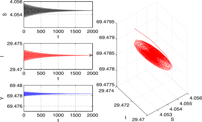
The trajectories of system (4.1) with \(\tau_{1}=5.79<\tau _{10}=5.8744, \tau_{2}=0\). The positive equilibrium E is asymptotically stable. The initial value is \((4,29.5,69.5)\)
Figure 3 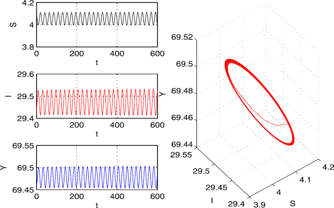
The trajectories of system (4.1) with \(\tau_{1}=5.88>\tau _{10}=5.8744, \tau_{2}=0\). A Hopf bifurcation occurs from the positive equilibrium E. The initial value is \((4,29.5,69.5)\)
-
(3)
When \(\tau_{1}>0\) and \(\tau_{2}>0\), let \(\tau_{1}=5.79\in (0,5.8744)\) and chose \(\tau_{2}\) as a parameter. Then the characteristic equation is
$$\begin{aligned} &\lambda^{3}+0.15\lambda^{2}+0.0054\lambda+4.0e{-}05+ \bigl(0.2906\lambda ^{2}+0.349\lambda+5.8151e{-}04\bigr)e^{-5.79\lambda}\\ &\qquad{}+ \bigl(0.2276\lambda ^{2}+0.0114\lambda+9.1054e{-}05\bigr)e^{-\lambda\tau_{2}}+(0.0649 \lambda +0.0013)e^{-\lambda(5.79+\tau_{2})}\\ &\quad=0. \end{aligned}$$


We obtain \(E_{43}=-1.3868e{-}06<0\), \(\omega^{*}_{20}=0.4438\), \(\tau ^{*}_{20}=4.5647\), and condition
- \((H_{5})\) :
-
\(Q_{31}Q_{33}+Q_{32}Q_{34}=0.0079\neq0\)
is satisfied. From Theorem 2.4 we know that the positive equilibrium E is asymptotically stable for \(\tau_{2}\in[0,\tau ^{*}_{20})\). As \(\tau_{2}\) continues to increase, the positive equilibrium E will lose stability, and a Hopf bifurcation occurs once \(\tau_{2}>\tau^{*}_{20}\). The corresponding numerical simulation results are shown Figs. 4–5.

The trajectories of system (4.1) with \(\tau_{1}=5.79, \tau _{2}=1<\tau^{*}_{20}=4.5647\). The positive equilibrium E is asymptotically stable. The initial value is \((4,29.5,69.5)\)

The trajectories of system (4.1) with \(\tau_{1}=5.79, \tau _{2}=5.2>\tau^{*}_{20}=4.5647\). A Hopf bifurcation occurs from the positive equilibrium E. The initial value is \((4,29.5,69.5)\)
Further, we get \(c_{1}(0)=-0.0055-0.005i, \mu_{2}=0.2471\), \(T_{2}=0.0044, \beta_{2}=-0.0111\). Therefore, from Theorem 3.1, we know that the Hopf bifurcation is supercritical and the bifurcating periodic solutions are stable.
5 Conclusion
In this paper, we study the dynamics of plant virus propagation model with two delays. First, we obtain sufficient conditions for the stability of positive equilibrium E and the existence of Hopf bifurcation when \(\tau_{1}>0, \tau_{2}=0\) and \(\tau_{1}\in(0,\tau _{10}), \tau_{2}>0, \tau_{1}\neq\tau_{2}\), respectively. Next, when \(\tau_{1}\neq\tau_{2}\), by using the center manifold and normal form theory, regarding \(\tau_{2}\) as a parameter, we investigate the direction and stability of the Hopf bifurcation. We derive an explicit algorithm for determining the direction of the Hopf bifurcation and the stability of the bifurcating periodic solutions. Finally, a numerical example supporting our theoretical predictions is given.
References
Jeger, M.J., van den Bosch, F., Madden, L.V., Holt, J.: A model for analysing plant-virus transmission characteristics and epidemic development. Math. Med. Biol. 15, 1–18 (1998)
Jeger, M.J., Madden, L.V., van den Bosch, F.: The effect of transmission route on plant virus epidemic development and disease control. J. Theor. Biol. 258, 198–207 (2009)
Varney, E.: Plant diseases: epidemics and control. Amer. J. Potato Res. 41(5), 153–154 (1964)
Jackson, M., Chen-Charpentier, B.M.: Modeling plant virus propagation with delays. J. Comput. Appl. Math. 309, 611–621 (2016)
Liu, J., Sun, L.: Dynamical analysis of a food chain system with two delays. Qual. Theory Dyn. Syst. 15, 95–126 (2016)
Shi, R., Yu, J.: Hopf bifurcation analysis of two zooplankton–phytoplankton model with two delays. Chaos Solitons Fractals 100, 62–73 (2017)
Deng, L., Wang, X., Peng, M.: Hopf bifurcation analysis for a ratio-dependent predator–prey system with two delays and stage structure for the predator. Appl. Math. Comput. 231, 214–230 (2014)
Wang, J., Wang, Y.: Study on the stability and entropy complexity of an energy-saving and emission-reduction model with two delays. Entropy 18(10), 371 (2016)
Ma, J., Si, F.: Complex dynamics of a continuous Bertrand duopoly game model with two-stage delay. Entropy 18(7), 266 (2016)
Zhang, Z., Wang, Y., Bi, D., et al.: Stability and Hopf bifurcation analysis for a computer virus propagation model with two delays and vaccination. Discrete Dyn. Nat. Soc. 2017, 1–17 (2017)
Han, Z., Ma, J., Si, F., et al.: Entropy complexity and stability of a nonlinear dynamic game model with two delays. Entropy 18(9), 317 (2016)
Dai, Y., Jia, Y., Zhao, H., et al.: Global Hopf bifurcation for three-species ratio-dependent predator–prey system with two delays. Adv. Differ. Equ. 2016, 13 (2016)
Liu, J.: Hopf bifurcation analysis for an SIRS epidemic model with logistic growth and delays. J. Appl. Math. Comput. 50, 557–576 (2016)
Zhang, Z., Hui, Y.: Ming, F.: Hopf bifurcation in a predator–prey system with Holling type III functional response and time delays. J. Appl. Math. Comput. 44, 337–356 (2014)
Song, Y.L., Peng, Y.H., Wei, J.J.: Bifurcations for a predator–prey system with two delays. J. Math. Anal. Appl. 337, 466–479 (2008)
Ruan, S.G., Wei, J.J.: On the zeros of transcendental functions with applications to stability of delay differential equations with two delays. Dyn. Contin. Discrete Impuls. Syst., Ser. A Math. Anal. 10, 863–874 (2003)
Kuznetsov, Y.A.: Elements of Applied Bifurcation Theory. Springer, New York (2004)
Hale, J.K.: Theory of Functional Differential Equations. Springer, New York (1977)
Hassard, B.D., Kazarinoff, N.D., Wan, Y.H.: Theory and Applications of Hopf Bifurcation. Cambridge University Press, Cambridge (1981)
Acknowledgements
The authors are grateful to the editor and anonymous reviewers for their valuable comments and suggestions.
Funding
Qinglian Li is supported by the National Natural Science Foundation of China (No. 11761040); Yunxian Dai is supported by the National Natural Science Foundation of China (No. 11761040 and No. 11461036).
Author information
Authors and Affiliations
Contributions
All authors contributed equally to the writing of this paper. All authors read and approved the final manuscript.
Corresponding author
Ethics declarations
Competing interests
The authors declare that they have no competing interests.
Additional information
Publisher’s Note
Springer Nature remains neutral with regard to jurisdictional claims in published maps and institutional affiliations.
Rights and permissions
Open Access This article is distributed under the terms of the Creative Commons Attribution 4.0 International License (http://creativecommons.org/licenses/by/4.0/), which permits unrestricted use, distribution, and reproduction in any medium, provided you give appropriate credit to the original author(s) and the source, provide a link to the Creative Commons license, and indicate if changes were made.
About this article

Cite this article
Li, Q., Dai, Y., Guo, X. et al. Hopf bifurcation analysis for a model of plant virus propagation with two delays. Adv Differ Equ 2018, 259 (2018). https://doi.org/10.1186/s13662-018-1714-8
Received:
Accepted:
Published:
DOI: https://doi.org/10.1186/s13662-018-1714-8