
Abstract
In this paper, we consider a two-dimensional predator-prey model with a time delay and square root response function. We analyze the stability of equilibria with the delay τ increasing and the critical value of τ when Hopf bifurcation occurs. Because the model has the term of square root, the zero point is a singularity. In order to clearly study the stability of the zero point, we rescale the variable \(x(t)\), say \(x(t)=X^{2}(t)\). The conclusion is that the zero point is not stable and the instability is not affected by the delay τ. We apply the normal form method and center manifold theorem to obtain the direction and stability of the Hopf bifurcation. Finally, we make several numerical simulations which is consistent with the conclusion of theoretical analysis.
1 Introduction
Dynamics of predator-prey models are one of the important subjects in ecology and mathematical ecology. Many researchers have studied predator-prey models with delay and derived some important results [1–9]. A few researchers have studied the model with the term of square root [10–12]. Braza [11] analyzed the following predator-prey model with square root response function:
where \(x(t)\) and \(y(t)\) denote the population (or density) of the prey and predator, respectively. s is the death rate of the predator, and c is the biomass conversion or consumption rate.
In system (1.1), \(x(t)\) stands for the number of prey without competition and predation, \(x^{2}(t)\) stands for the reduced number of competition of prey and prey, the term of \(\sqrt {x(t)}y(t)\) stands for the amount of assimilation by predator via competition of prey and predator [13], and \(sy(t)\) is the dead quantity of predator. Because the c is the consumption rate, and the term of \(\sqrt{x(t)}y(t)\) stands for the amount of assimilation by predator, the \(c\sqrt{x(t)}y(t)\) stands for the growth of predator via competition of prey and predator. In [10], Salman et al. have investigated the nonlinear dynamics of a discrete predator-prey model with square root functional response, obtained by applying a forward Euler discretization method to system (1.1). In [11], the dynamics of the square root system (1.1) are compared and contrasted with the dynamics of predator-prey systems that use a typical Lotka-Volterra interaction term. The process of growth needs time to finish, so in order to accurately express the model, we should add a time delay to the model, and system (1.1) becomes system (1.2) as follows:
Here, we assume the predator takes time τ to convert the food into its growth. By choosing τ as bifurcation parameter, we get the condition under which Hopf bifurcation occurs. At last we will give an example showing that the stability of the positive equilibrium will be changed with τ increasing.
This paper is organized as follows: In Section 2, we first focus on the stability of the equilibria and Hopf bifurcation by analyzing the eigenvalues. In Section 3, we derive the direction and stability of the Hopf bifurcation by using normal form method and central manifold theorem. In Section 4, a numerical simulation is made to examine the discussion of the previous section. A brief discussion is given in the last section.
2 Stability analysis and Hopf bifurcation
In this section, we research the stability of the equilibria and Hopf bifurcation by analyzing the eigenvalues of the system (1.2).
There are at most three nonnegative equilibria for system (1.2):
\(E^{*}_{3}\) is a unique positive equilibrium if and only if the following condition is true:
- \((H_{1})\) :
-
\(c>s\).
Let \(E^{*}=(x^{*},y^{*})\) be the arbitrary equilibrium, then the linearized system of (1.2) at \(E^{*}\) is
where \(u(t)=(x(t),y(t))^{T}\),
The characteristic determinant of system (2.1) is
The characteristic equation of system (2.1) is
In the following, we discuss the stability of the equilibria and Hopf bifurcation:
-
(1)
\(E^{*}=E^{*}_{1}=(0,0)\).
It is obvious that matrices (2.2) and (2.3) are indeterminate at \(E^{*}_{1}\). We rescale the variable \(x(t)\), say \(x(t)=X^{2}(t)\), so system (1.2) becomes the following form:
The characteristic equation of system (2.6) at \(E^{*}_{1}\) is
The eigenvalues of the characteristic equation (2.7) are \(\frac {1}{2}\) and −s; it is obvious that \(E^{*}_{1}\) is unstable. From equation (2.7), it is seen that the delay τ has no effect on the stability of \(E^{*}_{1}\).
-
(2)
\(E^{*}=E^{*}_{2}=(1,0)\).
The characteristic equation of system (2.1) is
The eigenvalues of the characteristic equation (2.8) are −1 and \(c-s\), so \(E^{*}_{2}\) is stable when \(s>c\) and unstable when \(s< c\). However, if the predator death rate s is larger than its consumption rate c, the predator will die out, leaving the prey to flourish. From equation (2.8), it can be seen that the delay τ has also no effect on the stability of \(E^{*}_{2}\).
-
(3)
\(E^{*}=E^{*}_{3}=(s^{2}/c^{2},s(c^{2}-s^{2})/c^{3})\).
In the following, we study the local stability of the positive equilibrium \(E^{*}_{3}\) by analyzing the distribution of the roots of equation (2.5). We consider two cases.
Case 1. When \(\tau=0\), the characteristic equation of system (2.1) is
From equation (2.9), we can see that when \(\frac{a_{11}+a_{22}}{2}<0\), \(\Delta =(a_{11}+a_{22})^{2}-4(a_{11}a_{22}-a_{12}b_{21})<0\), the two roots of equation (2.9) have always negative real parts; when \(\frac{a_{11}+a_{22}}{2}>0\), and \(\Delta<0\), the two roots of equation (2.9) have always negative real parts; when \(\frac{a_{11}+a_{22}}{2}>0\), and \(\Delta\geq0\), equation (2.9) has at least one positive root.
Let
- \((H_{2})\) :
-
\(\frac{a_{11}+a_{22}}{2}<0\), \(\Delta<0\);
- \((H_{3})\) :
-
\(\frac{a_{11}+a_{22}}{2}>0\).
Then it is not difficult to verify that the following result holds.
Lemma 2.1
For \(\tau=0\), the following statements are true:
-
(1)
If the conditions \((H_{1})\) and \((H_{2})\) hold, then \(E^{*}_{3}\) is stable.
-
(2)
If the conditions \((H_{1})\) and \((H_{3})\) hold, then \(E^{*}_{3}\) is unstable.
Case 2. When \(\tau>0\), the characteristic equation of system (2.1) is equation (2.5).
The equilibrium \(E^{*}_{3}\) is stable if all roots of (2.5) have negative real parts, thus we should observe the distribution of roots of equation (2.5). If iω (\(\omega>0\)) is a root of equation (2.5), ω should satisfy
Separating the real and imaginary parts, we have
which implies
Let \(z=\omega^{2}\) and denote
Then equation (2.12) becomes
Denote
we have
Assume that \((H_{1})\) holds, from (2.13) and (2.14), \(-\frac {p}{2}\leq0\) and \(q<0\), we know that equation (2.15) has one positive root for \(z\in(0,\infty)\). The positive root is denoted by \(z_{*}\). Equation (2.12) has a positive root denoted by \(\omega_{*}\), then \(\omega_{*}=\sqrt{z_{*}}\).
By (2.11), we have \(\cos \omega_{*}\tau_{*}=\frac{-\omega _{*}^{2}+a_{11}a_{22}}{a_{12}b_{21}}\).
Thus, if we denote
where \(j=0,1,2,\ldots \) , then \(\pm i\omega_{*}\) is a pair of purely imaginary roots of equation (2.5) with \(\tau_{*}^{(j)}\). Define
In order to investigate the distribution of the roots of equation (2.5), we need to introduce the following Lemma 2.2 from Ruan and Wei [14].
Lemma 2.2
Consider the exponential polynomial
where \(\tau_{i}\geq0\) (\(i=1,2,\ldots,m\)) and \(p_{j}^{(i)}\) (\(i=0,1,\ldots m;j=1,2,\ldots,n\)) are constants. As \((\tau_{1},\tau _{2},\ldots,\tau_{m})\) vary, the sum of the order of the zeros of \(p(\lambda,e^{-\lambda\tau _{1}},\ldots,e^{-\lambda\tau_{m}})\) on the open right half plane can change only if a zero appears on the imaginary axis.
Let \(\lambda(\tau)=\alpha(\tau)+i\omega(\tau)\) be the root of equation (2.5) near \(\tau=\tau_{*}^{(j)}\) satisfying
Then the following transversality condition holds.
Lemma 2.3
Suppose that \(z_{*}=\omega_{*}^{2}\), and \(h{'}(z_{*})\neq0\), then \(\frac{d(\operatorname{Re}\lambda(\tau _{*}^{(j)}))}{d\tau}\neq0\), and the sign of \(\frac{d(\operatorname{Re}\lambda(\tau_{*}^{(j)}))}{d\tau}\) is consistent with that of \(h{'}(z_{*})\).
Proof
Substituting \(\lambda(\tau)\) into equation (2.5) and differentiating the resulting equation in τ, we obtain
thus
where \(\tau=\tau_{*}^{(j)}\), \(\lambda=i\omega_{*}\),
From (2.18), (2.19) and (2.11), we obtain
where \(\Lambda= a_{12}^{2}b_{21}^{2}>0\). Thus, we have
Notice that \(\Lambda>0\), we conclude that the sign of \([\frac{\operatorname{Re}d \lambda(\tau)}{d \tau}]_{\tau=\tau_{*}^{(j)}}\) is determined by \(h{'}(z_{*})\). The proof is complete. □
Applying Lemmas 2.1-2.3, we get the following stability and bifurcation results for system (1.2).
Theorem 2.1
Suppose that \((H_{1})\) and \((H_{2})\) hold, then all roots of equation (2.5) have negative real parts for \(\tau\in[0,\tau _{*}^{(0)})\), the positive equilibrium \(E^{*}_{3}\) is asymptotically stable for \(\tau\in[0,\tau_{*}^{(0)})\) and the system (1.2) undergoes a Hopf bifurcation at \(E^{*}_{3}\) when \(\tau=\tau _{*}^{(j)}\) (\(j=0,1,2,\ldots \)).
Theorem 2.2
Suppose that \((H_{1})\) and \((H_{3})\) hold, then equation (2.5) has at least one root with positive real parts for \(\tau\in [0,\tau_{*}^{(0)})\), the positive equilibrium \(E^{*}_{3}\) is unstable for \(\tau\in[0,\tau_{*}^{(0)})\) and system (1.2) undergoes a Hopf bifurcation at \(E^{*}_{3}\) when \(\tau=\tau_{*}^{(j)}\) (\(j=0,1,2,\ldots\)).
3 Direction and stability of the Hopf bifurcation
In the second section, we got the condition of the system (1.2) appear as a Hopf bifurcation at \(\tau=\tau^{(j)} \) (\(j=0,1,2,\ldots\)). We determine the Hopf bifurcation direction and the properties of these bifurcating periodic solutions by using the normal form method and center manifold theorem.
Let \(x_{1}=x-x^{*}\), \(x_{2}=y-y^{*}\), \(\overline{x}_{i}(t)=x_{i}(\tau t)\), \(\tau=\tau_{*}^{(j)}+\mu\), where \(\tau_{*}^{(j)}\) is defined by (2.16). For convenience, drop the bar and let \(p(x)=\sqrt{x}\), then the system (1.2) can be written as an FDE in \(C=C([-1,0],R^{2})\) as
where \(x(t)=(x_{1}(t),x_{2}(t))^{T}\in R^{2}\) and \(L_{\mu }:C\rightarrow R^{2}\), \(f:R\times C\rightarrow R^{2}\) are given, respectively, by
and
where \(f_{1}=-\phi_{1}^{2}(0)-l_{1}\phi_{1}(0)\phi_{2}(0)-l_{2}\phi _{1}^{2}(0)\phi_{2}(0)-l_{3}\phi_{2}^{2}(0)+\cdots\), \(f_{2}=l_{4}\phi_{1}(-1)\phi_{2}(0)+l_{5}\phi_{1}^{2}(-1)\phi _{2}(0)+l_{6}\phi_{1}^{2}(-1)+\cdots\), and \(\phi(\theta)=(\phi_{1}(\theta),\phi_{2}(\theta))^{T}\in R^{2}\), \(l_{1}=p{'}(x^{*})\), \(l_{2}=\frac{p{''}(x^{*})}{2}\), \(l_{3}=\frac{p{''}(x^{*})y^{*}}{2}\), \(l_{4}=cp{'}(x^{*})\), \(l_{5}=\frac{cp{''}(x^{*})}{2}\), \(l_{6}=\frac{cp{''}(x^{*})y^{*}}{2}\).
In the previous section, we found that, in system (3.1), the Hopf bifurcation appears at \(\tau=\tau_{*}^{(0)}\). Next we will apply the Riesz representation theorem to analyze a function \(\eta(\theta,\mu)\).
In fact, we can choose
where δ is a Dirac-delta function. For \(\phi\in C^{1}([-1,0],R^{2})\), define
and
Then, when \(\theta=0\), system (3.1) is equivalent to
where \(x_{t}(\theta)=x(t+\theta)\) for \(\theta\in[-1,0)\). For \(\psi\in C^{1}([0,1],(R^{2})^{*})\), define
and a bilinear inner product
where \(\eta(\theta)=\eta(\theta,0)\). Denote \(A=A(0)\), then A and \(A^{*}\) are adjoint operators. By Theorem 2.1, we know that \(\pm i\omega_{0}\tau^{(j)} \) are eigenvalues of A.
which yields
Similarly, it can be verified that \(q^{*}(s)=D(1,\alpha^{*}) e^{is\omega_{0}\tau^{(j)}}\) is the eigenvector of \(A^{*}\) corresponding to \(-i\omega_{0}\tau^{(j)}\), where
By (3.7), we get
Thus, we obtain
such that \(\langle q^{*}(s),q(\theta)\rangle=1\). In the following, we will compute the coordinates which describe the center manifold \(C_{0}\) at \(\mu=0\) by using the same notations as the ideas in Hassard et al. [15]. Let \(x_{t}\) be the solution of equation (3.1) when \(\mu=0\). Define
On the center manifold \(C_{0}\), we have
where z and z̅ are local coordinates for center manifold \(C_{0}\) in the direction of q and q̅. Note that W is real if \(x_{t}\) is real. We consider only real solutions. For the solution \(x_{t}\in C_{0}\) of (3.1), since \(\mu =0\), we have
where
By (3.8), we have \(x_{t}(\theta)=(x_{1t}(\theta),x_{2t}(\theta ))^{T}=W(t,\theta)+z q(\theta)+\overline{z}\overline{q}(\theta)\), and then
It follows together with (3.3) that
Comparing the coefficients with (3.12), we have
In order to determine \(g_{21}\), in the sequel, we need to compute \(W_{20}(\theta)\) and \(W_{11}(\theta)\). From (3.6) and (3.8), we have
where
Notice that near the origin on the center manifold \(C_{0}\), we have
thus
Since (3.11) holds, for \(\theta\in[-1,0)\), we have
Comparing the coefficients with (3.12) gives
From (3.14), (3.15) and the definition of A, we get
Notice that \(q(\theta)=q(0)e^{i\tau^{(j)}\omega_{0}\theta}\). We have
where \(E_{1}=(E_{1}^{(1)}, E_{1}^{(2)}) \in R^{2}\) is a constant vector. In the same way, we also obtain
where \(E_{2}=(E_{2}^{(1)}, E_{2}^{(2)}) \in R^{2}\) is also a constant vector. In what follows, we will seek appropriate \(E_{1}\) and \(E_{2}\). From the definition of A and (3.14), we obtain
and
where \(\eta(\theta)=\eta(0,\theta)\). From (3.11) and (3.12), we have
and
Substituting (3.17) and (3.21) into (3.19) and noticing that
and
we obtain
which leads to
It follows that
where
Similarly, substituting (3.18) and (3.22) into (3.20), we get
Thus, we have
where
Firstly, we determine \(g_{20}\), \(g_{11}\), \(g_{02}\), then we can determine \(E_{1}\) and \(E_{2}\). Next, we can determine \(W_{20}\) and \(W_{11}\). Finally, we can determine \(g_{21}\). Thus it is easy to compute the following values:
which determine the quantities of bifurcating periodic solutions in the center manifold at the critical value \(\tau^{(j)}\). Suppose \(\operatorname{Re}\{\lambda{'}(\tau^{{(j)}})\}>0\). \(\mu_{2}\) determines the directions of the Hopf bifurcation: if \(\mu_{2}>0\) (<0), then the Hopf bifurcation is supercritical (subcritical) and the bifurcation exists for \(\tau>\tau^{(j)}\) (\(<\tau^{(j)}\)). \(\beta_{2}\) determines the stability of the bifurcation periodic solutions: the bifurcating periodic solutions are stable (unstable) if \(\beta_{2}<0\) (>0). And \(T_{2}\) determines the period of the bifurcating periodic solutions: the period increases (decreases) if \(T_{2}>0\) (<0).
4 Numerical simulation
In this section, we make numerical simulations to examine the conclusion of the previous sections. We might as well consider the following system:
System (4.1) has a positive equilibrium \(E^{*}_{3}(0.36,0.384)\), and the characteristic equation of system (4.1) at \(E^{*}_{3}\) is
Next, we analyze the stability of the positive equilibrium \(E^{*}_{3}(0.36,0.384)\) with τ increasing by several figures.
-
(1)
When \(\tau=0\), from the Routh-Hurwitz criterion, it is obvious that \(E^{*}_{3}(0.36,0.384)\) is stable. This agrees with Figure 1.
Figure 1 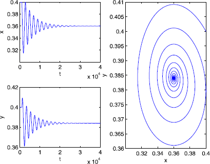
The trajectories of system ( 4.1 ) with \(\pmb{\tau=0}\) . The positive equilibrium \(E^{*}_{3}\) is asymptotically stable.

Since \(-\frac{p}{2}\), \(q<0\), from Theorem 2.1, it is obvious that the positive equilibrium \(E^{*}_{3}\) of equation (4.1) is stable for \(\tau\in[0,\tau_{*}^{(0)})\).
Now, we will choose two appropriate values of τ to verify.
From the discussion of Section 2, we get
-
(2)
When \(\tau=0.2\), it is obvious that \(E^{*}_{3}(0.36,0.384)\) is asymptotically stable (see Figure 2).
Figure 2 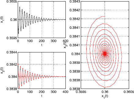
The trajectories of system ( 4.1 ) with \(\pmb{\tau =0.2}\) . The positive equilibrium \(E^{*}_{3}\) is asymptotically stable.
-
(3)
When \(\tau=0.44\), a periodic solution bifurcates from the equilibrium \(E^{*}_{3}(0.36,0.384)\) in Figure 3.
Figure 3 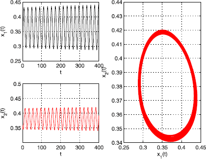
The trajectories of system ( 4.1 ) with \(\pmb{\tau =0.44}\) . A periodic solution bifurcates from the equilibrium \(E^{*}_{3}\).


From the discussion of Section 3, we also get a series of data:
Since \(\mu_{2}>0\), \(\beta_{2}<0\), the bifurcating periodic solution from the positive equilibrium \(E^{*}_{3}\) is supercritical and asymptotically stable at \(\tau=\tau_{*}^{(0)}\).
5 Conclusion
In this paper, a predator-prey model with a time delay and square root response function is considered. Taking the time delay as bifurcating parameter, the stability of the equilibria and the existence of Hopf bifurcation is discussed. It is shown that the stability of \(E^{*}_{1}=(0,0)\) and \(E^{*}_{2}=(1,0)\) have not changed as the delay τ increases. We have also obtained the conditions at which system (1.2) undergoes a Hopf bifurcation at the positive equilibrium \(E^{*}_{3}\). By using the center manifold theory and normal form method, the direction and stability of the Hopf bifurcation are determined. The results of our numerical simulations are in agreement with the theoretical findings.
References
Zhao, HT, Lin, YP, Dai, YX: Bifurcation analysis and control of chaos for a hybrid ratio-dependent three species food chain. Appl. Math. Comput. 218, 1533-1546 (2011)
Song, Y, Xiao, W, Qi, XY: Stability and Hopf bifurcation of a predator-prey model with stage structure and time delay for the prey. Nonlinear Dyn. 83, 1409-1418 (2016)
Zhang, CQ, Liu, LP, Yan, P, Zhang, LZ: Stability and Hopf bifurcation analysis of a predator-prey model with time delayed incomplete trophic transfer. Acta Math. Appl. Sin. Engl. Ser. 31(1), 235-246 (2015)
Wang, WY, Pei, LJ: Stability and Hopf bifurcation of a delayed ratio-dependent predator-prey system. Acta Mech. Sin. 27(2), 285-296 (2011)
Wang, LS, Feng, GH: Stability and Hopf bifurcation for a ratio-dependent predator-prey system with stage structure and time delay. Adv. Differ. Equ. 2015, Article ID 255 (2015)
Yang, RZ: Bifurcation analysis of a diffusive predator-prey system with Crowley-Martin functional response and delay. Chaos Solitons Fractals 95, 131-139 (2017)
Yang, RZ, Zhang, CR: Dynamics in a diffusive modified Leslie-Gower predator-prey model with time delay and prey harvesting. Nonlinear Dyn. 87, 863-878 (2016)
Yang, RZ, Zhang, CR: Dynamics in a diffusive predator-prey system with a constant prey refuge and delay. Nonlinear Anal., Real World Appl. 31, 1-22 (2016)
Yang, RZ, Liu, M, Zhang, CR: A diffusive toxin producing phytoplankton model with maturation delay and three-dimensional patch. Comput. Math. Appl. 73, 824-837 (2017)
Salman, SM, Yousef, AM, Elsadany, AA: Stability, bifurcation analysis and chaos control of a discrete predator-prey system with square root functional response. Chaos Solitons Fractals 93, 20-31 (2016)
Braza, PA: Predator-prey dynamics with square root functional responses. Nonlinear Anal., Real World Appl. 13, 1837-1843 (2012)
Moreno, M, Platania, F: A cyclical square-root model for the term structure of interest rates. Eur. J. Oper. Res. 241, 109-121 (2015)
Ajraldi, V, Pittavino, M, Venturino, E: Modeling herd behavior in population systems. Nonlinear Anal., Real World Appl. 12, 2319-2338 (2011)
Ruan, SG, Wei, JJ: On the zeros of transcendental function with applications to stability of delay differential equations with two delays. Dyn. Contin. Discrete Impuls. Syst., Ser. A Math. Anal. 10, 863-874 (2003)
Hassard, BD, Kazarinoff, ND, Wan, Y: Applications of Hopf Bifurcation. Cambridge University Press, Cambridge (1981)
Acknowledgements
We are grateful to the editors and the anonymous referees for their careful reading and constructive suggestions which lead to truly significant improvement of the manuscript. This research is supported by the National Natural Science Foundation of China (No. 11061016 and No. 11561034).
Author information
Authors and Affiliations
Corresponding author
Additional information
Competing interests
The authors declare that they have no competing interests.
Authors’ contributions
All authors contributed equally to the writing of this paper. All authors read and approved the final manuscript.
Publisher’s Note
Springer Nature remains neutral with regard to jurisdictional claims in published maps and institutional affiliations.
Rights and permissions
Open Access This article is distributed under the terms of the Creative Commons Attribution 4.0 International License (http://creativecommons.org/licenses/by/4.0/), which permits unrestricted use, distribution, and reproduction in any medium, provided you give appropriate credit to the original author(s) and the source, provide a link to the Creative Commons license, and indicate if changes were made.
About this article

Cite this article
Zhu, X., Dai, Y., Li, Q. et al. Stability and Hopf bifurcation of a modified predator-prey model with a time delay and square root response function. Adv Differ Equ 2017, 235 (2017). https://doi.org/10.1186/s13662-017-1292-1
Received:
Accepted:
Published:
DOI: https://doi.org/10.1186/s13662-017-1292-1