
Abstract
Even though the effect of release frequency of green lacewings in controlling the spread of mealybugs in a cassava field was investigated by Promrak and Rattanakul in 2015, the effect of increased global temperature was not taken into account. In this work, cellular automata and Monte Carlo simulation are employed in order to study the effect of an increased global temperature on the life cycles of mealybugs and green lacewings which in turn effects the efficacy of the biological control of the spread of mealybugs. Computer simulations are carried out at different temperatures so that an efficient biological control of the spread of mealybugs in a cassava field is obtained.
1 Introduction
The term ‘global warming’ refers to an increase in the average temperature of Earth’s atmosphere and oceans. According to the report from Goddard Institute for Space Studies (GISS) and Climatic Research Unit (CRU), the temperature has been increasing almost every year since 1880 and has climbed up fast in the last few decades. The Intergovernmental Panel on Climate Change (IPCC) forecasts that, for the next two decades, a further warming trend will occur at the rate 0.1-0.2∘C per decade. Global warming may cause several severe problems such as the increase in the spread of insect-borne diseases, heavier rainfall and flooding, food and water deficiency, season changing and migration [1]. On crops and insect pests, the increase in the global temperature may lead to the change in the life cycle of insect pests at any stage and the rate of pest development might be higher while the host plants are more attractive to insect pests in drought areas [2, 3]. As a result, the loss of crop yields will then increases.
Under the global increased temperature condition, crops which can thrive in hot and dry climates such as cassava is considered as a key for food security. Cassava (Manihot esculenta Crantz) is also known as yuca, manioc, tapioca, mandioc, etc. Its root and tuber are the main source of food for Africans and are popular in the tropics [4]. Since it requires little skill to cultivate with moderate soil nutrient and water, this crop is very attractive to agriculturists worldwide [5]. In 2005, the top importers of cassava are East Asia (US$460,070,000), EU25 (US$59,534,000), and NAFTA (US$48,725,000) while the primary exporters are South East Asia (US$533,926,000), Central America (US$66,173,000), and EU25 (US$ 7,853,000) [6]. For Thailand, the cassava export of the year 2015 has been reported as 79.56% of the global market share [7]. Therefore, cassava is considered as an economic plant of Thailand.
The major crop loss of cassava is due to its insect pests, especially cassava mealybug (Phenacoccus manihoti Matile-Ferrero) which was first detected in Zaire and Congo in the early 1970s and quickly became the most severe pest on cassava [8]. To control the spread of mealybugs, biological control using their natural enemies has proved experimentally to be successful [9–14]. One of the natural enemies of mealybugs that has been used popularly is green lacewings. It has been used in a mealybug controlling project in Thailand [15, 16] as well. However, various instructions are recommended to farmers in Thailand when the spread of mealybugs is detected. Moreover, the effect of an increased global temperature on the life cycles of both mealybugs and green lacewings has not been taken into account yet.
In our previous work [17], a cellular automata (CA) model together with the Monte Carlo simulation technique has been employed to study the effect of the release frequency of green lacewings in controlling the spread of mealybugs in a cassava field [17]. Since the effect of an increased global temperature on the life cycles of mealybugs and green lacewings should be investigated so that we can appropriately modify the usual practices in the control of the spread of mealybugs in response to those changes, we investigate the effect of an increased temperature on the controlling of the spread of mealybugs in a cassava field using green lacewings in this paper.
2 Cellular automata model
We assume that cassava is planted in the field based on the recommended instructions of the Department of Agricultural Extension, Ministry of Agriculture and Cooperatives, Thailand. Cassava is then planted at the beginning of the rainy season and the stem cuttings are soaked by the recommended chemical reactants before they are planted in the cassava field. Hence, the major factor of the spread of mealybugs in the field that we will take into account is the wind. Note that only mealybugs of the instar stage can be blown by the wind. Moreover, the recommended planting distance between two cassava plants is 1 m and the planting period of cassava is 1 year. We also assume further that the survey for the spread of mealybugs will be conducted every 2 weeks after a month of planting in the recommended manner by many agricultural technical officers from the Thai Tapioca Development Institute and the Department of Agriculture, Ministry of Agriculture and Cooperatives, Thailand [18].
A cellular automaton with Moore’s neighborhood of a square lattice with the size \(80\times80\) is used to represent a cassava field of the area 4 rai (or 0.64 ha) as shown in Figure 1. The possible states of each cell in the lattice are susceptible cassava (S), infested cassava (I) and removed cassava (E) representing a cassava plant that is free from mealybugs, a cassava plant that is infested with mealybugs and a cassava plant that is removed from the field, respectively.

A lattice representing a cassava field.
At each time step (1 time step \(\Delta t=1\) day), a number r, \(0\leq r\leq1\) is randomized and each cell will be updated at random according to the following rules:
-
(a)
If the randomized cell is a removed cassava (E), then it remains the removed cassava.
-
(b)
If the randomized cell is a susceptible cassava (S), then there are possibilities that the randomized cell may become an infested cassava (I) due to the following reasons:
-
(i)
Mealybugs of the instar stage from outside of the cassava field might be blown through the wind to the randomized cell. If the randomized cell belongs to the first two rows next to each of the four borders of the lattice then the cell may become an infested cell with the probability \(w_{1}\), \(0\leq w_{1}\leq1\) or else the randomized cell may become an infested cell with the probability \(w_{2}\), \(0\leq w_{2} < w_{1}\leq1\).
-
(ii)
Mealybugs of the instar stage from the neighborhood of the randomized might be blown through the wind to the randomized cells. Here, we consider only three levels of neighborhood of the randomized cell which are the immediate neighborhood, the distant neighborhood and the far distant neighborhood as shown in Figure 2. The probabilities that mealybugs of the instar stage from the immediate neighborhood, distant neighborhood and far distant neighborhood might be blown through the wind to the randomized cells are \(n_{1}\), \(n_{2}\) and \(n_{3}\), respectively, where \(0\leq n_{3} < n_{2} < n_{1}\leq1\).
Figure 2 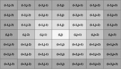
Neighborhoods of the updating cell \(\pmb{(i,j)}\) . The light gray, gray and dark gray areas represent immediate neighborhood, distant neighborhood and far distant neighborhood, respectively.
-
(i)
-
(c)
If the randomized cell is an infested cassava (I), then the following rules will be used.
-
(i)
It may become a removed cassava (E) if it is subjected to a survey during the first 4 months or the last 5 months of planting or the number of mealybugs on the randomized cell is greater than \(m_{1}\).
-
(ii)
It may become a susceptible cassava (S) if green lacewings feed on mealybugs on the cassava plant in the randomized cell successfully and there is no mealybug on the cassava plant in the randomized cell.
-
(i)

When a month has passed after cassava planting, if there is an infested cassava plant among the surveyed cassava plants, green lacewings are to be released every 2 months if there still are mealybugs on the surveyed cassava plants in the field. If the number of surveyed infested cassava plants is less than a half of the total number of surveyed cassava plants in the field, the number of green lacewings to be released in the field is \(R_{1}\) per rai (or \(R_{1}/0.16\) per ha) or else the number of green lacewings to be released in the field is \(R_{2}\) per rai (or \(R_{2}/0.16\) per ha).
In what follows, we let \(P^{i}_{t}\), \(P^{m}_{t}\), \(P^{e}_{t}\) be the number of instar mealybugs, adult mealybugs and mealybug’s eggs, respectively, at time t. Let \(M^{i}_{t}\), \(M^{d}_{t}\), \(M^{m}_{t}\) and \(M^{e}_{t}\) be the number of larva green lacewings, pupa green lacewings, adult green lacewings and green lacewings’ egg, respectively, at time t. The numbers of mealybugs and green lacewings at each stage on the cassava plant in each cell of the lattice are also updated according to the life cycles of mealybugs and green lacewings using a system of difference equations as follows.
- Instar mealybug: :
-
$$\begin{aligned} P^{i}_{t+\Delta t} =&P^{i}_{t}+r_{1} \alpha_{1} P^{e}_{t}-\alpha_{2} P^{i}_{t}-\beta _{1}\bigl(P^{i}_{t},M^{i}_{t} \bigr)M^{i}_{t} . \end{aligned}$$(1)
Equation (1) represents the number of instar mealybugs at the time step \(t+\Delta t\). The first term on the right hand side represents the number of instar mealybugs at the time step t. The second term on the right hand side represents the number of instar mealybugs developed from mealybug’s egg of the time step t. The third term on the right hand side represents the number of instar mealybugs of the time step t that develop into adult mealybugs in the time step \(t+\Delta t\). The last term on the right hand side represents the number of instar mealybugs eaten by green lacewings of the larva stage in the time step t.
- Adult mealybug: :
-
$$\begin{aligned} P^{m}_{t+\Delta t} =&P^{m}_{t}+r_{2} \alpha_{2} P^{i}_{t}-\alpha_{3} P^{m}_{t}-\beta _{2}\bigl(P^{m}_{t},M^{i}_{t} \bigr)M^{i}_{t}. \end{aligned}$$(2)
Equation (2) represents the number of adult mealybugs at the time step \(t+\Delta t\). The first term on right hand side represents the number of adult mealybugs at the time step t. The second term on the right hand side represents the number of adult mealybugs developed from instar mealybug of the time step t. The third term on the right hand side represents the number of adult mealybugs of the time step t that die in the time step \(t+1\) due to mealybug’s life cycle. The last term on the right hand side represents the number of adult mealybugs eaten by green lacewings of the larva stage in the time step t.
- Mealybug’s egg: :
-
$$\begin{aligned} P^{e}_{t+\Delta t} =&P^{e}_{t}+r_{3} \alpha_{4} v_{1} P^{m}_{t}- \alpha_{1} P^{e}_{t}-\beta _{3} \bigl(P^{e}_{t},M^{i}_{t} \bigr)M^{i}_{t}. \end{aligned}$$(3)
Equation (3) represents the number of mealybug’s eggs at the time step \(t+\Delta t\). The first term on the right hand side represents the number of mealybug’s eggs at the time step t. The second term on the right hand side represents the number of mealybug’s eggs laid by adult mealybugs of the time step t. The third term on the right hand side represents the number of mealybug’s eggs in the time step t that develop into instar mealybugs in the time step \(t+\Delta t\). The last term on the right hand side represents the number of mealybug’s eggs eaten by green lacewings of the larva stage in the time step t.
- Larva green lacewing: :
-
$$\begin{aligned} M^{i}_{t+\Delta t} =&M^{i}_{t}+s_{1} \gamma_{1} M^{e}_{t}-\gamma_{2} M^{i}_{t} . \end{aligned}$$(4)
Equation (4) represents the number of larva green lacewings at the time step \(t+\Delta t\). The first term on the right hand side represents the number of larva green lacewings at the time step t. The second term on the right hand side represents the number of larva green lacewings developed from green lacewing’s eggs of the time step t. The last term on the right hand side represents the number of larva green lacewings in the time step t that develop into pupa green lacewings in the time step \(t+\Delta t\).
- Pupa green lacewing: :
-
$$\begin{aligned} M^{d}_{t+\Delta t} =&M^{d}_{t}+s_{2} \gamma_{2} \delta_{1}\bigl(P^{i}_{t},P^{m}_{t},P^{e}_{t},M^{i}_{t} \bigr) M^{i}_{t}-\gamma_{3} M^{d}_{t} . \end{aligned}$$(5)
Equation (5) represents the number of pupa green lacewings at the time step \(t+\Delta t\). The first term on the right hand side represents the number of pupa green lacewings at the time step t. The second term on the right hand side represents the number of pupa green lacewings developed from larva green lacewings of the time step t depending on the number of consumed mealybugs. The last term on the right hand side represents the number of pupa green lacewings in the time step t that develop into adult green lacewings in the time step \(t+\Delta t\).
- Adult green lacewing: :
-
$$\begin{aligned} M^{m}_{t+\Delta t} =&M^{m}_{t}+s_{3} \gamma_{3} M^{d}_{t}-\delta_{2} M^{m}_{t} . \end{aligned}$$(6)
Equation (6) represents the number of adult green lacewings at the time step \(t+\Delta t\). The first term on the right hand side represents the number of adult green lacewings at the time step t. The second term on the right hand side represents the number of adult green lacewings developed from pupa green lacewings of the time step t. The last term on the right hand side represents the number of adult green lacewings of the time step t that die in the time step \(t+\Delta t\) due to green lacewing’s life cycle.
- Green lacewing’s eggs: :
-
$$\begin{aligned} M^{e}_{t+\Delta t} =&M^{e}_{t}+s_{4} v_{2} M^{m}_{t}-\gamma_{1} M^{e}_{t}. \end{aligned}$$(7)
Equation (7) represents the number of green lacewing’s eggs at the time step \(t+\Delta t\). The first term on the right hand side represents the number of green lacewing’s eggs at the time step t. The second term on the right hand side represents the number of green lacewing’s eggs laid by adult green lacewings of the time step t. The last term on the right hand side represents the number of green lacewing’s eggs in the time step t that develop into larva green lacewings in the time step \(t+\Delta t\).
\(\beta_{1} (P^{i}_{t}, M^{i}_{t} )\), \(\beta_{2} (P^{m}_{t}, M^{i}_{t} )\) and \(\beta_{3} (P^{e}_{t}, M^{i}_{t} )\) are the numbers of instar mealybugs, adult mealybugs and mealybug’s eggs eaten by green lacewings of the larva stage, respectively, in one time step and \(\delta_{1} (P^{i}_{t},P^{m}_{t},P^{e}_{t},M^{i}_{t} )\) is the efficiency of converting larva green lacewing to pupa green lacewing. The definitions of other parameters in the model are given in Table 1 together with their approximated values calculated from the literature [19–21] at three different temperatures.
Furthermore, the approximated total crop yield is also monitored. We also assume that the estimated crop yield is a kilograms per cassava plant if there is no mealybug in the cassava field. The estimated crop yield will be reduced by 100%, 30% and 10%, approximately, if mealybugs spread on the cassava plants during the first 4 months, during the 5th and the 7th month, and during the 8th and the 12th month, respectively, according to the surveys of the Thai Tapioca Development Institute in 2007-2010. Hence, the estimated crop yield at each time step, \(Y(t)\), is then assumed to be represented by the following equation:
where \(C_{1}\) is the total number of susceptible cassava at the time step t, \(C_{2}\) is the total number of cassava infested by mealybugs during the 8th and the 12th month at the time step t and \(C_{3}\) is the total number of cassava infested by mealybugs during the 5th and the 7th month at the time step t.
3 Simulation results
In this section, numerical simulations at the three different temperatures 25∘C, 27∘C and 30∘C are carried out in order to investigate the effect of increased temperatures on the control of mealybugs.
When biological control is applied, we assume that the survey for the spread of mealybugs will be done every two weeks beginning one month after planting as recommended by many agricultural technical officers from the Thai Tapioca Development Institute and the Department of Agriculture, Ministry of Agriculture and Cooperatives, Thailand. According to the recommendation of the Department of Agricultural Extension, Ministry of Agriculture and Cooperatives, Thailand, the cassava field will be surveyed by collecting the numbers of mealybugs at all stages on the cassava plants that are not planted on the two rows next to the four borders of the cassava field. The survey will be conducted on every two rows of plants, and every 11 plants. On the cassava field of the size 80 m × 80 m with 1 m between two cassava plants, a cassava plant might be surveyed with the probability
Flow charts of the simulations are given in Figures 3-9. The results shown in Figures 10-15 are the averaged values of the 100 runs using MATLAB software. In the simulations, the parameters in the system of difference equations (1)-(7) are as in Table 1 where \(n_{1}=0.05\), \(n_{2}=0.005\), \(n_{3}=0.0005\), \(w_{1}=0.001\), \(w_{2}=0.0001\), \(a=2.25\), \(R_{1}=800\), \(R_{2}=1{,}000\) and

The main loop of CA.

The main susceptible cassava updating loop.

The neighborhood checking loop of the susceptible cassava updating loop.

The main infested cassava updating loop.

The number of mealybugs updating loop (incorporating wind effect) of infested cassava.

The neighborhood checking loop of the number of mealybugs updating loop (incorporating wind effect) of the infested cassava.

The green lacewings releasing loop.

The average number of susceptible cassava at \(\pmb{25^{\circ}\mbox{C}}\) , \(\pmb{27^{\circ}\mbox{C}}\) and \(\pmb{30^{\circ}\mbox{C}}\) . (a) No biological control is applied, (b) larva green lacewings are released in the cassava field, (c) adult green lacewings are released in the cassava field.
First, we investigate the spread of mealybugs when there is no biological control, when larva green lacewings are released to control the spread of mealybugs and when adult green lacewings are released to control the spread of mealybugs. The number of susceptible cassava plants, the number of infested cassava plants, the number of removed cassava plants and the estimated crop yield at 25∘C, 27∘C and 30∘C are as shown in Figures 10, 11, 12 and 13.

The average number of infested cassava at \(\pmb{25^{\circ}\mbox{C}}\) , \(\pmb{27^{\circ}\mbox{C}}\) and \(\pmb{30^{\circ}\mbox{C}}\) . (a) No biological control is applied, (b) larva green lacewings are released in the cassava field, (c) adult green lacewings are released in the cassava field.

The average number of removed cassava at \(\pmb{25^{\circ}\mbox{C}}\) , \(\pmb{27^{\circ}\mbox{C}}\) and \(\pmb{30^{\circ}\mbox{C}}\) . (a) No biological control is applied, (b) larva green lacewings are released in the cassava field, (c) adult green lacewings are released in the cassava field.

The average estimated cassava’s crop yield at \(\pmb{25^{\circ}\mbox{C}}\) , \(\pmb{27^{\circ}\mbox{C}}\) and \(\pmb{30^{\circ}\mbox{C}}\) . (a) No biological control is applied, (b) when larva green lacewings are released in the cassava field, (c) adult green lacewings are released in the cassava field.
Next, the total numbers of larva and adult green lacewings that are released to control the spread of mealybugs in a cassava field at 25∘C, 27∘C and 30∘C are presented in comparison as shown in Figure 14. Moreover, the number of instar mealybugs when there is no biological control, when larva green lacewings are released to control the spread of mealybugs and when adult green lacewings are released to control the spread of mealybugs at 25∘C, 27∘C and 30∘C are also shown in Figure 15.

The total numbers of green lacewings that are released to control the spread of mealybugs in a cassava field at \(\pmb{25^{\circ}\mbox{C}}\) , \(\pmb{27^{\circ}\mbox{C}}\) and \(\pmb{30^{\circ}\mbox{C}}\) . (a) Larva green lacewings are released in the cassava field, (b) adult green lacewings are released in the cassava field.

The average numbers of instar mealybugs at \(\pmb{25^{\circ}\mbox{C}}\) , \(\pmb{27^{\circ}\mbox{C}}\) and \(\pmb{30^{\circ}\mbox{C}}\) . (a) No biological control is applied, (b) larva green lacewings are released in the cassava field, (c) adult green lacewings are released in the cassava field.
We can see from the simulation results that even though the average numbers of instar mealybugs is very high when a biological control is applied, the number of the infested cassava plants is not that high. This means that the spread of mealybugs can be controlled to be located on only a small number of cassava plants although the number of mealybugs might be high on those cassava plants. Here, snapshots showing the distribution of susceptible cassava, infested cassava and removed cassava in the cassava field of a simulation at 30∘C are also given in Figures 16 and 17 for a better understanding.

Snapshots showing the distribution of susceptible cassava, infested cassava and removed cassava in the cassava field of a simulation at \(\pmb{30^{\circ}\mbox{C}}\) on the 125th day of planting. (a) No biological control is applied, (b) larva green lacewings are released in the cassava field, (c) adult green lacewings are released in the cassava field.

Snapshots showing the distribution of susceptible cassava, infested cassava and removed cassava in the cassava field of a simulation at \(\pmb{30^{\circ}\mbox{C}}\) on the 285th day of planting. (a) No biological control is applied, (b) larva green lacewings are released in the cassava field, (c) adult green lacewings are released in the cassava field.
4 Discussion and conclusion
The increase in global temperatures affects the sex ratio, survival rate, reproduction rate and life cycle of both mealybugs and green lacewings. Simulations of the spread of mealybugs in a cassava field at 25∘C, 27∘C and 30∘C have been carried out.
Without biological control, the estimated crop yield decreases dramatically and tends to zero at 25∘C, and at 27∘C approximately 4 months after planting. At 30∘C, the estimated crop yield decreases and tends to a constant level which is lower than 30% of the maximum estimated crop yield.
With biological control, green lacewings at the larva stage or adult stage may be released in the cassava field to control the spread of mealybugs. Hence, we study both manners of biological control. We can see that the number of infested cassava plants decreases whereas the number of susceptible cassava plants increases when the temperature increases which might be the results of shorter life cycle, lower survival rate, lower fecundity and shorter adult longevity of mealybugs. We can also see that the release of green lacewing larva gives a better result when there is a spread of mealybugs even though the lower amount of larva green lacewing is released compared to adult green lacewings. The reasons for this might be the shorter life span, lower survival rate, lower fecundity or shorter adult longevity of green lacewings because only green lacewings at the larva stage behave like a predator of mealybugs and if we release adult green lacewings it will take a period of time before they will lay eggs which develop into green lacewing larva, finally behaving like a predator of mealybugs. With the increase of temperature, the survival rate and the fecundity rate are even lower and hence the greater amount of adult green lacewings should be released in the cassava field to control the spread of mealybugs. On the other hand, the estimated crop yield also increases when the temperature increases with the same level of released green lacewings. This implies that if farmers are satisfied with the estimated crop yield at the end of planting period when the temperature is 25∘C, they might reduce the number of green lacewings released in the cassava field so that the cost for biological control will be decreased and the farmers then earn more profit. On the other hand, if the farmers would like to gain more estimated crop yield at the end of planting period, they might keep the released amount of green lacewings at the same level as they use when the temperature is 25∘C. However, the cost for a green lacewings is approximately 0.50 baht (US$0.015) while the selling price for cassava is quite low, approximately 2.50 baht (US$0.072) per kilogram. Hence, the cost of biological control and the increase in crop yield should be calculated in order to obtain the most efficient biological control that maximizes profit.
References
Union of Concerned Scientists: Global warming impacts. http://www.ucsusa.org/our-work/global-warming/science-and-impacts/global-warming-impacts#.WS6Pe-Hfw-U
Sharma, HC, Prabhakar, CS: Impact of climate change on pest management and food security. In: Integrated Pest Management, pp. 23-36. Elsevier, Amsterdam (2014). http://www.sciencedirect.com/science/article/pii/B9780123985293000038
Fuhrer, J: Agroecosystem responses to combinations of elevated CO2, ozone, and global climate change. Agric. Ecosyst. Environ. 97, 1-20 (2003)
Deutsche, GTZ, Stumpf, E: Postharvest loss due to pests in dried cassava chips and comparative methods for its assessment: a case study on small-scale farm households in Ghana. Dissertation (1998). http://www.fao.org/wairdocs/x5426E/x5426e02.htm#1.%20introduction
Economic importance of cassava. http://plantbiostudy.blogspot.com/2013/09/economic-importance-of-cassava.html
Trade and Industrial Policy Strategies (TIPS), Australian Agency for International Development (AUSAID): Trade information brief - cassava. http://www.sadctrade.org/files/Cassava-Trade-Information-Brief.pdf
The situation of cassava trade in the world. http://thaitribune.org/contents/detail/340?content_id=16778&rand=1452192136
Neuenschwander, P: Control of the cassava mealybug in Africa: lessons from a biological control project. Afr. Crop Sci. J. 2(4), 369-383 (1994)
Chakupurakal, J, Markham, RH, Neuenschwander, P, Sakala, M, Malambo, C, Mulwanda, D, Banda, E, Chalabesa, A, Bird, T, Haug, T: Biological control of the cassava mealybug, Phenacoccus manihoti (Homoptera: Pseudococcidae), in Zambia. Biol. Control 4(3), 254-262 (1994)
Sarkar, MA, Suasa-Ard, W, Uraichuen, S: Host stage preference and suitability of Allotropa suasaardi Sarkar & Polaszek (Hymenoptera: Platygasteridae), a newly identified parasitoid of pink cassava mealybug, Phenacoccus manihoti (Homoptera: Pseudococcidae). Songklanakarin J. Sci. Technol. 37(4), 381-387 (2015)
Fernandes, MHA, Oliveira, JEM, Costa, VA, De Menezes, KO: Coccidoxenoides perminutus parasitizing Planococcus citri on vine in Brazil. Ciênc. Rural 46(7), 1130-1133 (2016)
Erkilic, LB, Demirbas, H, Güven, B: Citrus mealybug, biological control strategies and large scale implementation on citrus in Turkey. Acta Hortic. 1065, 1157-1164 (2015)
Marras, PM, Cocco, A, Muscas, E, Lentini, A: Laboratory evaluation of the suitability of vine mealybug, Planococcus ficus, as a host for Leptomastix dactylopii. Biol. Control 95, 57-65 (2016)
Beltrà, A, Soto, A, Tena, A: How a slow-ovipositing parasitoid can succeed as a biological control agent of the invasive mealybug Phenacoccus peruvianus: implications for future classical and conservation biological control programs. BioControl 60(4), 473-484 (2015)
Choeikamhaeng, P, Vinothai, A, Sahaya, S: Utilization of green lacewing Plesiochrysa ramburi for control cassava mealybugs in field. Department of Agricultures research database, Thailand (2011)
Suasa-ard, W: Natural enemies of important insect pests of field crops and utilization as biological control agents in Thailand. In: Proceedings of International Seminar on Enhancement of Functional Biodiversity Relevant to Sustainable Food Production in ASPAC, pp. 9-11 (2010)
Promrak, J, Rattanakul, C: Simultion study of the spread of mealybugs in a cassava field: effect of release frequency of a biological control agent. Kasetsart J. Natur. Sci. 49, 963-970 (2015)
Field Crops Research Institute, Department of Agricultural Extension, Ministry of Agriculture and Cooperatives, Thailand: Cassava producing technique…to stand up to cassava disaster (2014). agrimedia.agritech.doae.go.th/book/book-rice/RB%20043.pdf
Chong, JH, Roda, AL, Mannion, CM: Life history of the mealybug, Maconellicoccus hirsutus (Hemiptera: Pseudococcidae), at constant temperatures. Environ. Entomol. 37, 323-332 (2008)
Pappas, ML, Broufas, GD, Koveos, DS: Effect of prey availability on development and reproduction of the predatory lacewing Dichochrysa prasina (Neuroptera: Chrysopidae). Ann. Entomol. Soc. Am. 102, 437-444 (2009)
Pappas, ML, Koveos, DS: Life-history traits of the predatory lacewing Dichochrysa prasina (Neuroptera: Chrysopidae): temperature-dependent effects when larvae feed on nymphs of Myzus persicae (Hemiptera: Aphididae). Ann. Entomol. Soc. Am. 104, 43-49 (2011)
Acknowledgements
This work was supported by the Development and Promotion of Science and Technology Talents Project (DPST), the Centre of Excellence in Mathematics, Thailand, The Thailand Research Fund and Mahidol University, Thailand (contract number RSA5880004).
Author information
Authors and Affiliations
Corresponding author
Additional information
Competing interests
The authors declare that they have no competing interests.
Authors’ contributions
The first author carried out a numerical investigation of the developed model and the second author developed the model and carried out numerical investigations. All authors read and approved the final manuscript.
Publisher’s Note
Springer Nature remains neutral with regard to jurisdictional claims in published maps and institutional affiliations.
Rights and permissions
Open Access This article is distributed under the terms of the Creative Commons Attribution 4.0 International License (http://creativecommons.org/licenses/by/4.0/), which permits unrestricted use, distribution, and reproduction in any medium, provided you give appropriate credit to the original author(s) and the source, provide a link to the Creative Commons license, and indicate if changes were made.
About this article

Cite this article
Promrak, J., Rattanakul, C. Effect of increased global temperatures on biological control of green lacewings on the spread of mealybugs in a cassava field: a simulation study. Adv Differ Equ 2017, 161 (2017). https://doi.org/10.1186/s13662-017-1218-y
Received:
Accepted:
Published:
DOI: https://doi.org/10.1186/s13662-017-1218-y