
Abstract
We consider the geometric inverse problem of determining an immersed obstacle in a two-dimensional non-stationary Stokes fluid flow. We use the topological gradient method to solve this problem. The unknown obstacle is located and reconstructed using the leading term of the Khon–Vogelius shape function variation. We propose a simple and fast detection algorithm. The efficiency and accuracy of the proposed approach are illustrated by some numerical examples.
1 Introduction
In this work, we study the problem of detecting submerged obstacles in a viscous fluid in the case where the movement of the fluid is governed by the unsteady Stokes equations. Here we want to detect the position and reconstruct the shape of an unknown obstacle (can be defined by multiple components) from boundary measurements. The unknown obstacle \(\mathcal{Q}^{*}\) is assumed to be located in a larger area in which a viscous, incompressible, and non-stationary fluid flows. We then perform a measurement on \(\varGamma_{a}\) a part of the boundary ∂Ω (i.e., on the surface of the fluid Ω) (see Fig. 1).

Study case
To reconstruct the obstacle, we define a cost form functional allowing the error between the real solution (through the measurement) and the approximate solution to be evaluated. We are working here with the Kohn–Vogelius type functional [1] which rephrases the geometric inverse problem into a shape optimization one. The objective is to minimize these functionals using an optimization algorithm in order to get closer to the real solution. For the minimization procedure, we use the topological asymptotic analysis technique [2–7].
This problem has been studied in the case of stationary Stokes flow [8–10]. This work corresponds to the time dependent case. We begin by describing the used technique in Sect. 2. The theoretical result associated with the topological asymptotic expansion is presented in Sect. 3. In the last section, we propose a numerical investigation. A numerical algorithm is presented and used for different cases in order to illustrate the efficiency of the proposed method.
2 Problem formulation
Let Ω be a bounded domain of \(\mathbb{R}^{2}\) containing an obstacle \(\mathcal{Q}^{*}\) and \(\partial\varOmega=\varGamma_{i}\cup\varGamma_{a}\) be its boundary.
This paper is concerned with the following geometric inverse problem:
Knowing Neumann and Dirichlet data on an accessible part \(\varGamma_{a}\) of the boundary; an imposed force F and a measured velocity field \(\mathcal{U}_{m}\) on \(\varGamma_{a}\) such that \(\varGamma_{a} \subset\partial\varOmega\) and \(\operatorname{mes}(\varGamma _{a} )\neq0\).
Detect the location and the shape of the unknown obstacles \(\mathcal{Q}^{*}\) such that the solution \(({\mathbf{u}}_{\mathcal{Q}^{*}}, p_{\mathcal{Q}^{*}})\) of the non-stationary Stokes equations satisfies the following over-determined boundary value problem:
$$ \textstyle\begin{cases} \frac{\partial{\mathbf{u}}_{\mathcal{Q}^{*}}}{\partial t}-\nu \Delta{\mathbf{u}}_{\mathcal{Q}^{*}}+\nabla p_{\mathcal{Q}^{*}} = \mathbf{G} & \mbox{in } \varOmega \setminus \overline{{\mathcal{Q}^{*}}}\times\,]0,T[, \\ \operatorname{div} {\mathbf{u}}_{\mathcal{Q}^{*}} = 0 & \mbox{in } \varOmega \setminus \overline{{\mathcal{Q}^{*}}}\times\,]0,T[, \\ \sigma({\mathbf{u}}_{\mathcal{Q}^{*}}, p_{\mathcal{Q}^{*}}) . \mathbf{n} = \mathbf{F} & \mbox{on } \varGamma_{a}\times\,]0,T[, \\ {\mathbf{u}}_{\mathcal{Q}^{*}} = \mathcal{U}_{m} & \mbox{on } \varGamma_{a}\times\,]0,T[, \\ {\mathbf{u}}_{\mathcal{Q}^{*}} = 0 & \mbox{on } \varGamma_{i} \times\,]0,T[, \\ {\mathbf{u}}_{\mathcal{Q}^{*}} = 0 & \mbox{on } \partial \mathcal{Q}\times\,]0,T[, \\ {\mathbf{u}}_{\mathcal{Q}^{*}}(\cdot,0) = {\mathbf{u}}^{0}& \mbox{in } \varOmega \setminus \overline{{\mathcal{Q}^{*}}}, \end{cases} $$where ν is the kinematic viscosity coefficient of the fluid, G is the gravitational force, \({\mathbf{u}}^{0}\) is the initial fluid flow velocity, \(\sigma({\mathbf{u}}_{\mathcal{Q}^{*}}, p_{\mathcal{Q}^{*}}):=( \nabla\mathbf{u}_{\mathcal{Q}^{*}} + \nabla\mathbf{u}_{ \mathcal{Q}^{*}} ^{T} ) -p_{\mathcal{Q}^{*}} \mathbf{I}\), and n is the outside unit normal vector at ∂Ω.
In this work, we propose a reconstruction approach based on the Kohn–Vogelius formulation and the topological gradient method.
Let \(\mathcal{Q}\subset\varOmega\) be an arbitrary obstacle. The Kohn–Vogelius function is defined by
where \({\mathbf{u}}_{\mathcal{Q}}^{N}\) and \({\mathbf{u}}_{\mathcal{Q}}^{D}\) are respectively solutions of the following unsteady Stokes problems:
and
One can observe that if \(\mathcal{Q}\) coincides with the exact obstacle \(\mathcal{Q}^{*}\), then \({\mathbf{u}}_{\mathcal{Q}}^{D}={\mathbf{u}}_{\mathcal{Q}}^{N}\). Starting from this observation, the inverse problem can be formulated as follows:
where \(\mathcal{D}_{\mathrm{ad}}\) is a given set of admissible domains.
To solve problem (4) and detect the location of the unknown obstacle \(\mathcal{Q}^{*}\), we use the topological sensitivity analysis method [11–15]. It consists in determining the asymptotic development of the solution of the considered non-stationary Stokes problem when we add a small obstacle inside the domain Ω. We deduce a characterization of the topological derivative of the Kohn–Vogelius functional \(\mathcal{K}\). We can then minimize it to solve our initial inverse problem using a gradient optimization algorithm. The use of this notion of topological gradient makes it possible to determine the number of objects present and their approximate positions.
The idea of using the topological derivative is as follows. We consider the Kohn–Vogelius functional \(\mathcal{K}\) in the case of unsteady Stokes equations presented above (see (1)). For a small parameter \(\varepsilon>0\) and a point \(\mathbf{z} \in\varOmega\), we consider a perturbed domain \(\varOmega\setminus\overline{\mathcal{Q}_{\mathbf{z}, \varepsilon}}\) created by inserting a small obstacle (will be modeled by a small hole) inside the initial domain Ω near the point z such that \(\mathcal{Q}_{\mathbf{z}, \varepsilon}=\mathbf{z} +\varepsilon \mathcal{Q}\), where \(\mathcal{Q}\) is a given, fixed, and bounded domain of \(\mathbb{R}^{2}\) containing the origin.
We then begin by studying the influence of the modification of the topology on the variations of \(\mathcal{K}\). One can usually obtain an asymptotic development of the functional \(\mathcal{K}\) of the following form:
where ρ is a positive scalar function tending to 0 with ε and \(\delta \mathcal{K}\) is called the topological gradient (or topological derivative). It provides information on the insertion of a small hole at point z which corresponds to the point where \(\mathcal{K}\) reaches its minimum.
3 Asymptotic development
In this work, we extend the sensitivity analysis approach to the non-stationary regime, and we derive a topological asymptotic expansion for the considered Kohn–Vogelius shape function.
In the presence of a small obstacle \(\mathcal{Q}_{\mathbf{z}, \varepsilon}=\mathbf{z}+\varepsilon \mathcal{Q}\), the function \(\mathcal{K}\) is defined by
with
\(({\mathbf{u}}_{\varepsilon}^{N}, p_{\varepsilon}^{N})\) is the solution to the perturbed Neumann problem
$$ \bigl(\mathcal{P}^{N}_{\varepsilon}\bigr) \textstyle\begin{cases} \frac{\partial{\mathbf{u}}_{\varepsilon}^{N} }{\partial t}-\nu \Delta{\mathbf{u}}_{\varepsilon}^{N}+\nabla p_{\varepsilon}^{N} = \mathbf{G} & \mbox{in } \varOmega \setminus \overline{\mathcal{Q}_{\mathbf{z}, \varepsilon}}\times\,]0,T[, \\ \operatorname{div} {\mathbf{u}}_{\varepsilon}^{N} = 0 & \mbox{in } \varOmega \setminus \overline{\mathcal{Q}_{\mathbf{z}, \varepsilon}}\times\,]0,T[, \\ \sigma({\mathbf{u}}_{\varepsilon}^{N},p_{\varepsilon}^{N}) .\mathbf {n} = \mathbf{F} & \mbox{on } \varGamma_{a}\times\,]0,T[, \\ {\mathbf{u}}_{\varepsilon}^{N} = 0 & \mbox{on } \varGamma _{i}\times\,]0,T[, \\ {\mathbf{u}}_{\varepsilon}^{N} = 0 & \mbox{on } \partial \mathcal{Q}_{\mathbf{z}, \varepsilon}\times\,]0,T[, \\ {\mathbf{u}}_{\varepsilon}^{N}(\cdot,0) = {\mathbf{u}}^{0} & \mbox{in } \varOmega \setminus \overline{\mathcal{Q}_{\mathbf{z}, \varepsilon}}. \end{cases} $$\(({\mathbf{u}}_{\varepsilon}^{D}, p_{\varepsilon}^{D})\) is the solution to the perturbed Dirichlet problem
$$ \bigl(\mathcal{P}^{D}_{\varepsilon}\bigr) \textstyle\begin{cases} \frac{\partial{\mathbf{u}}_{\varepsilon}^{D} }{\partial t}-\nu \Delta{\mathbf{u}}_{\varepsilon}^{D}+\nabla p_{\varepsilon}^{D} = \mathbf{G} & \mbox{in } \varOmega \setminus \overline{\mathcal{Q}_{\mathbf{z}, \varepsilon}}\times\,]0,T[, \\ \operatorname{div} {\mathbf{u}}_{\varepsilon}^{D} = 0 & \mbox{in } \varOmega \setminus \overline{\mathcal{Q}_{\mathbf{z}, \varepsilon}}\times\,]0,T[, \\ {\mathbf{u}}_{\varepsilon}^{D} = \mathcal{U}_{m} & \mbox{on } \varGamma_{a}\times\,]0,T[, \\ {\mathbf{u}}_{\varepsilon}^{D} = 0 & \mbox{on } \varGamma _{i}\times\,]0,T[, \\ {\mathbf{u}}_{\varepsilon}^{D} = 0 & \mbox{on } \partial \mathcal{Q}_{\mathbf{z}, \varepsilon}\times\,]0,T[, \\ {\mathbf{u}}_{\varepsilon}^{D}(\cdot,0) = {\mathbf{u}}^{0} & \mbox{in } \varOmega \setminus \overline{\mathcal{Q}_{\mathbf{z}, \varepsilon}}. \end{cases} $$
The Kohn–Vogelius functional \(\mathcal{K}\) satisfies the following theorem (see [16] for the proof).
Theorem 1
Let\(\mathcal{Q}_{\mathbf{z}, \varepsilon}\)be a small obstacle inserted in the fluid flow domainΩ. Then the Kohn–Vogelius functional\(\mathcal{K}\)admits the following topological asymptotic expansion:
where\(\delta \mathcal{K}\)is the topological gradient defined by
In the last expression
\(\mathbf{ u}^{D}_{0}\) and \(\mathbf{u}^{N}_{0}\) are respectively solutions of problems \((\mathcal{P}^{D}_{\varepsilon})\) and \((\mathcal{P}^{N}_{\varepsilon})\) for \(\varepsilon=0\).
\(\varPhi_{0}^{N}\) is the Neumann adjoint state, solution to
$$ \bigl(\mathcal{A}^{N}\bigr) \textstyle\begin{cases} - \frac{\partial\varPhi_{0}^{N} }{\partial t}-\nu \Delta\varPhi_{0}^{N}+\nabla\pi_{0}^{N} =- D\mathcal{F}({ \mathbf{u}}^{N}_{0}-{\mathbf{u}}^{D}_{0}) & \mbox{in } \varOmega\times\,]0,T[, \\ \operatorname{div} \varPhi_{0}^{N} = 0 & \mbox{in } \varOmega\times\,]0,T[, \\ \sigma(\varPhi_{0}^{N},\pi_{0}^{N}) n = 0 & \mbox{on } \varGamma_{a} \times\,]0,T[, \\ \varPhi_{0}^{N} = 0 & \mbox{on } \varGamma_{i}\times\,]0,T[, \\ \varPhi_{0}^{N}(\cdot,T) = 0 & \mbox{in } \varOmega. \end{cases} $$\(\varPhi_{0}^{D}\) is the Dirichlet adjoint state, solves
$$ \bigl(\mathcal{A}^{D}\bigr) \textstyle\begin{cases} - \frac{\partial\varPhi_{0}^{D} }{\partial t}-\nu \Delta\varPhi_{0}^{D}+\nabla\pi_{0}^{D} =- D\mathcal{F}({ \mathbf{u}}^{D}_{0}-{\mathbf{u}}^{N}_{0}) & \mbox{in } \varOmega\times\,]0,T[, \\ \operatorname{div} \varPhi_{0}^{D} = 0 & \mbox{in } \varOmega\times\,]0,T[, \\ \varPhi_{0}^{D} = 0 & \mbox{on } \varGamma_{a}\times\,]0,T[, \\ \varPhi_{0}^{D} = 0 & \mbox{on } \varGamma_{i}\times\,]0,T[, \\ \varPhi_{0}^{D}(\cdot,T) = 0 & \mbox{in } \varOmega. \end{cases} $$Here, \(\mathcal{F}\) is the cost function defined on \(H^{1}(\varOmega)^{2}\) by
$$ \mathcal{F}(w)= \int_{\varOmega} \bigl\vert \nabla w(\mathbf{x}) \bigr\vert ^{2}\, d \mathbf{x} . $$
4 Numerical results
In this section, we reconstruct numerically one (or more) small submerged obstacle in a non-stationary fluid when the movement of the fluid is governed by the incompressible non-stationary Stokes equations. We use the topological derivative of the Kohn–Vogelius functional presented in Theorem 1 to solve the minimization problem (4). We begin by validating the asymptotic behavior established in Theorem 1. Then, we present a numerical algorithm to detect the unknown obstacles with different forms from over-determined boundary data. The numerical simulations presented here are made in two dimensions using the finite elements library Freefem++ [17].
4.1 Numerical validation of the asymptotic expansion
To validate the theoretical asymptotic expansion established in Theorem 1, we introduce the function \(\Delta_{\mathbf{z}}( \varepsilon)\) defined by
We study the variation of this function with respect to ε for different locations of obstacles \(\mathcal{Q}_{\mathbf{z}_{i}, \varepsilon}= \mathbf{z}_{i} + \varepsilon B(0,1) \), \(i=1, \ldots, 4\). The coordinates \(\mathbf{z}_{i}= (x_{i}, y_{i})\) of considered obstacles are described in Table 1. We expect to prove numerically that \(\Delta_{\mathbf{z}_{i}}(\varepsilon)\) satisfies the obtained theoretical estimate \(\Delta_{\mathbf{z}_{i}}(\varepsilon)= o ( \frac{-1}{ \log( \varepsilon)} ) \).
Let \(\alpha_{i}\) be such that \(\Delta_{\mathbf{z}_{i}}(\varepsilon)= O ((- \log(\varepsilon) )^{ \alpha_{i}} )\). In Fig. 2, we illustrate the variation of the function \(\log( | \Delta_{\mathbf{z}_{i}}(\varepsilon) | )\) with respect to \(\log( - \log(\varepsilon))\). Then \(\alpha_{i}\) is the slope of the line approximating the variation \(\varepsilon\mapsto\log( | \Delta_{\mathbf{z}_{i}}(\varepsilon) | )\) with respect to \(\log( - \log(\varepsilon))\).

Variation of \(\log ( \vert \Delta_{\mathbf{z}_{i}}(\varepsilon) \vert )\) with respect to \(\log (-\log(\varepsilon) )\)
The obtained slopes are presented in Table 2. They confirm the behavior predicted by the theoretical estimate.
4.2 Reconstruction procedure from boundary measurement
We present in this section a numerical algorithm for detecting the unknown obstacle \(\mathcal{Q}\) inserted inside the fluid flow domain Ω from over-determined data on Γ. Next, we present some reconstruction results obtained in one iteration, showing the efficiency and accuracy of our approach.
4.2.1 Identification procedure
The used numerical procedure is based on the asymptotic formula described by Theorem 1. The unknown object \(\mathcal{Q}\) is likely to be located at the zone where the topological gradient \(\delta \mathcal{K}\) is most negative. The obstacle shape will be reconstructed using a level set curve of a scalar function.
Let \(\delta_{\mathrm{min}}\) be the most negative value of the function \(\delta \mathcal{K}\) in the domain Ω, i.e.,
For each \(\beta\in[0, 1]\), we denote by \(\mathcal{Q}_{\beta}\) the subset of Ω defined by
The proposed numerical algorithm is based on the following steps.
Reconstruction algorithm
-
Solve the two problems (\(\mathcal{P}_{0}^{N}\)) and (\(\mathcal{P}_{0}^{D}\)).
-
Solve the two adjoint problems \((\mathcal{A}^{N})\) and \((\mathcal{A}^{D})\).
-
Compute the topological gradient \(\delta \mathcal{K}\).
-
Reconstruct the unknown obstacle \(\mathcal{\mathcal{Q}}^{*}\):
find \(\beta^{*}\in[0, 1]\) such that \(\mathcal{K}(\varOmega\setminus\overline{\mathcal{\mathcal{Q}}_{\beta^{*}}}) \leq \mathcal{K}(\varOmega\setminus\overline{\mathcal{\mathcal{Q}}_{\beta}})\), \(\forall \beta\in[0, 1]\);
set \(\mathcal{\mathcal{Q}}^{*} = \{ \mathbf{x}\in\varOmega; \mbox{such that } \delta \mathcal{K}(\mathbf{x}) \leq\beta^{*} \delta _{\mathrm{min}} \} \).
This one-iteration procedure has already been illustrated in [18] for the identification of cracks from over-determined boundary data and in [11, 19] for the detection of small gas bubbles in stationary Stokes flow. Next, we will apply this reconstruction algorithm for the non-stationary Stokes case.
In the following, we describe some reconstruction results obtained by the presented numerical algorithm for different test cases. The considered fluid domain Ω is defined by the square \([0,1]\times[0,1]\).
4.2.2 Influence of the shape of the obstacle
First, we suppose that the true obstacle is centered at \((0.5,0.5)\). We study the influence of the shape of the obstacle immersed inside the fluid flow domain on the efficiency of the detection.
- (a)
Elliptical shape
In Fig. 3, we present the reconstruction results for circular and elliptical shaped unknown obstacles. The exact geometry (to be reconstructed) is described by a black line. As one can see, the unknown obstacle is located at the negative zone and well approximated by a level set curve of the topological gradient \(\delta \mathcal{K}\). In the circular case, we have \(\delta_{\mathrm{min}} = -0.015\) and the reconstructed obstacle is obtained using \(\beta^{*}=0.96\). For the elliptical case, we have used \(\delta_{\mathrm{min}} = -0.08\) and \(\beta^{*}=0.977\).
Figure 3 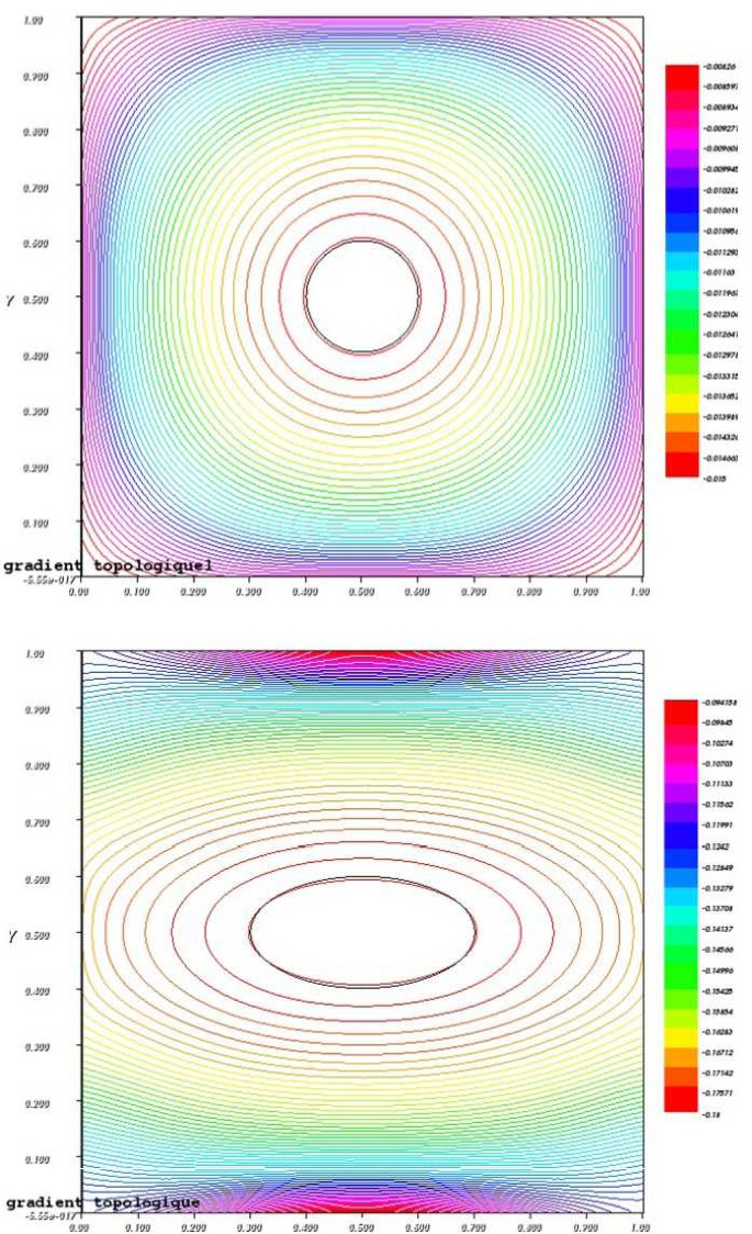
Reconstruction of circle and ellipse shapes
- (b)
Shape with corners
In the case of an obstacle with irregular boundary (with corners), our one-iteration algorithm can identify efficiently the location of this unknown obstacle but not its exact shape (see Fig. 4).
Figure 4 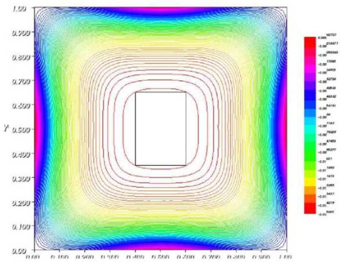
Reconstruction of shape with corners
- (c)
Nontrivial shape
In Fig. 5, we illustrate the case of a complex regular geometry. As one can observe, the reconstruction result for this nontrivial shape is quite good. In fact, we detect the location of the unknown obstacle but not its shape. The obtained result can serve as a good initial guess for an iterative optimization process based on the shape derivative.
Figure 5 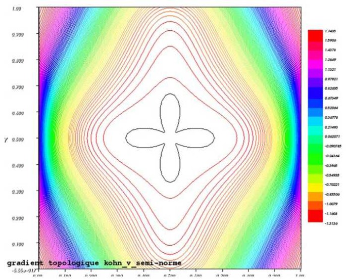
Reconstruction of a complex shape


In conclusion of these first simulations, as we expected, our one-iteration algorithm permits to reconstruct the location of the unknown obstacle that we have to determine and its rough shape in the case of elliptical shapes. Moreover, the location detection is efficient for different types of shapes, including shapes with corners.
4.2.3 Effect of the location of the obstacle
We consider a circular obstacle \(\mathcal{Q}=B(\mathbf{z}^{*},r^{*})\) centered at \(\mathbf{z}^{*}\) and having a fixed radius \(r^{*}=0.1\). The aim of this numerical experiment is to study the effect of the obstacle location on the reconstruction results.
We remark that the detection of obstacle location is efficient (see Fig. 6). For the shape, the result is good when the obstacle is not close enough to the boundary of the domain.

Reconstruction of a circular shape: effect of the location
4.2.4 Effect of the size of the obstacle
Here we consider two cases: The first one is a circular obstacle \(\mathcal{Q}=B(z^{*},r^{*})\) centered at \(\mathbf{z}^{*}=(0.4,0.4)\) and having variable radius \(r_{i}^{*}\), \(i=1,\ldots,6\) (see Fig. 7). The aim here is to discuss the effect of the size of the obstacle on the reconstruction results. These simulations show that if the characteristic size of the object becomes too large, the method becomes not precise enough. These results are not surprising since the smallness assumption is an essential argument to obtain the asymptotic expansion result presented in Theorem 1 and used in the numerical algorithm.

Reconstruction of a circular shaped obstacle: effect of the size
4.2.5 Sensitivity to the relative position of two obstacles
We consider two circular obstacles \(\mathcal{Q}_{1}=B(\mathbf{z}^{*}_{1},r^{*})\) and \(\mathcal{Q}_{2}=B(\mathbf{z}^{*}_{2},r^{*})\) having the same size \(r^{*}=0.05\) and separated by a variable distance d. Our aim here is to study the effect of the parameter \(\rho=d/r^{*}\).
We remark that the two obstacles are accurately detected when they are well-separated (see Fig. 8(a)). When the obstacles are close enough, the algorithm detects only a single area containing the two obstacles (see Fig. 8(c)).

Isovalues of the topological gradient showing the obtained obstacle locations
4.2.6 Effect of the relative size of two obstacles
This test is devoted to studying the relative size effect of two obstacles. We consider here two circular obstacles \(\mathcal{Q}^{*}_{1}=B(\mathbf{z}^{*}_{1},r^{*}_{1})\) and \(\mathcal{Q}^{*}_{2}=B(\mathbf{z}^{*}_{2},r^{*}_{2})\) separated by a fixed distance and having a different radius \(r^{*}_{1}\) and \(r^{*}_{2}\) with \(r^{*}_{1}=0.05 \leq r^{*}_{2}\). Here we study the effects of the parameter \(\mathcal{R}=r^{*}_{2}/r^{*}_{1}\) on the detection result.
We observe in Fig. 9 that the bigger obstacle is much better located than the small one; however, the identification process is sensitive to the relative size of the two obstacles. When the ratio \(\mathcal{R}\) decreases the information seems to be “captured” only by the biggest one as it can be viewed in Fig. 9(d).

Effect of the size of the two unknown obstacles
5 Conclusion
The numerical study of the obstacle detection in a non-stationary fluid flow has been performed. The used technique consists in studying the asymptotic expansion of the Khon–Vogelius function with respect to small perturbations of the domain. A fast and accurate algorithm is proposed and used for different configuration cases. The presented numerical simulations show the efficiency of the suggested approach.
References
Caubet, F., Dambrine, M., Kateb, D., Timimoun, Z.: Formulation to detect an obstacle immersed in a fluid. Inverse Probl. Imaging 7(1), 123–157 (2013)
Masmoud, M.: The topological asymptotic. In: Kawarada, H., Périaux, J. (eds.) Computational Method for Control Applications. International Series GAKUTO (2002)
Garreau, S., Guillaume, P., Masmoudi, M.: The topological asymptotic for PDE systems: the elasticity case. SIAM J. Control Optim. 39(6), 1756–1778 (2001)
Guillaume, P., Idris, K.S.: The topological asymptotic expansion for the Dirichlet problem. SIAM J. Control Optim. 41(4), 1042–1072 (2002)
Guillaume, P., Idris, K.S.: Topological sensitivity and shape optimization for the Stokes equations. SIAM J. Control Optim. 43(1), 1–31 (2004)
Abdelwahed, M., Al Salam, A., Chorfi, N.: Topological sensitivity analysis of a time-dependent nonlinear problem. Bound. Value Probl. 2019, 23 (2019)
Abdelwahed, M., Chorfi, N., Malek, R.: Reconstruction of Tesla micro-valve using topological sensitivity analysis. Adv. Nonlinear Anal. 9(1), 567–590 (2020)
Hassine, M.: Shape optimization for the Stokes equations using topological sensitivity analysis. ARIMA 5, 216–229 (2006)
Caubet, F., Dambrine, M.: Localization of small obstacles in Stokes flow. Inverse Probl. 28(10), 105007 (2012)
Antontsev, S., Shmarev, S.: On a class of fully nonlinear parabolic equations. Adv. Nonlinear Anal. 8(1), 79–100 (2019)
Badra, M., Caubet, F., Dambrine, M.: Detecting an obstacle immersed in a fluid by shape optimization methods. Math. Models Methods Appl. Sci. 21(10), 2069–2101 (2011)
Amstutz, S.: The topological asymptotic for the Navier–Stokes equations. ESAIM Control Optim. Calc. Var. 11(3), 401–425 (2005)
Abdelwahed, M., Hassine, M.: Topological optimization method for a geometric control problem in Stokes flow. Appl. Numer. Math. 23, 1–12 (2009)
Hassine, M., Masmoudi, M.: The topological asymptotic expansion for the quasi-Stokes problem. ESAIM Control Optim. Calc. Var. 10(4), 478–504 (2004)
Sokolowski, J., Zochowski, A.: On the topological derivative in shape optimization. SIAM J. Control Optim. 37, 1241–1272 (1999)
Malek, R., Abdelwahed, M., Chorfi, N., Hassine, M.: Geometric inverse problem for the non-stationary Stokes equations using topological sensitivity analysis. Math. Models Methods Appl. Sci. (2020, to appear)
Hecht, F.: Finite element library freefem++. http://www.freefem.org/ff++/
Andrieux, S., Baranger, T.N., Ben Abda, A.: Solving Cauchy problems by minimizing an energy-like functional. Inverse Probl. 22, 115–134 (2006)
Ben Abda, A., Hassine, M., Jaoua, M., Masmoudi, M.: Topological sensitivity analysis for the location of small cavities in Stokes flow. SIAM J. Control Optim. 48(5), 2871–2900 (2009)
Acknowledgements
The authors would like to extend their sincere appreciation to the Deanship of Scientific Research at King Saud University for funding this Research group No. (RG-1440-061).
Availability of data and materials
Not applicable.
Funding
Not applicable.
Author information
Authors and Affiliations
Contributions
The authors declare that the study was realized in collaboration with equal responsibility. All authors read and approved the final manuscript.
Corresponding author
Ethics declarations
Competing interests
The authors declare that they have no competing interests.
Additional information
Publisher’s Note
Springer Nature remains neutral with regard to jurisdictional claims in published maps and institutional affiliations.
Rights and permissions
Open Access This article is licensed under a Creative Commons Attribution 4.0 International License, which permits use, sharing, adaptation, distribution and reproduction in any medium or format, as long as you give appropriate credit to the original author(s) and the source, provide a link to the Creative Commons licence, and indicate if changes were made. The images or other third party material in this article are included in the article’s Creative Commons licence, unless indicated otherwise in a credit line to the material. If material is not included in the article’s Creative Commons licence and your intended use is not permitted by statutory regulation or exceeds the permitted use, you will need to obtain permission directly from the copyright holder. To view a copy of this licence, visit http://creativecommons.org/licenses/by/4.0/.
About this article

Cite this article
Malek, R., Abdelwahed, M., Chorfi, N. et al. Obstacle detection in fluid flow using asymptotic analysis technique. Bound Value Probl 2020, 45 (2020). https://doi.org/10.1186/s13661-020-01347-y
Received:
Accepted:
Published:
DOI: https://doi.org/10.1186/s13661-020-01347-y