
Abstract
Background
The aim was to develop statistical shape models of the main human tarsal bones that would result in novel representations of cuboid, navicular and talus.
Methods
Fifteen right and 15 left retrospectively collected computed tomography data sets from male individuals, aged from 17 to 63 years, with no known foot pathology were collected. Data were gathered from 30 different subjects. A process of model building includes image segmentation, unifying feature position, mathematical shape description and obtaining statistical shape geometry.
Results
Orthogonal decomposition of bone shapes utilising spherical harmonics was employed providing means for unique parametric representation of each bone. Cross-validated classification results based on parametric spherical harmonics representation showed high sensitivity and high specificity greater than 0.98 for all considered bones.
Conclusions
The statistical shape models of cuboid, navicular and talus created in this work correspond to anatomically accurate atlases that have not been previously considered. The study indicates high clinical potential of statistical shape modelling in the characterisation of tarsal bones. Those novel models can be applied in medical image analysis, orthopaedics and biomechanics in order to provide support for preoperative planning, better diagnosis or implant design.
Background
The statistical shape model (SSM) has been established as a powerful tool for medical image analysis [1–6]. The goal of constructing a statistical shape model is to obtain a mean shape and description of variation from a collection of samples [7–10]. The methods employed strongly depend on the chosen shape representation, which can be landmarks and meshes, medial models, Fourier surfaces, spherical harmonics, deformable models, wavelets description, non-uniform rational B-Splines and others [11, 12]. The choice of the shape representation influences further processing and calculation and in that context landmark-based point distribution models have become popular and commonly used methods. Statistical shape models are usually used for the task of segmentation [13, 14], but they could also be considered for finite element (FE) modelling [15, 16] and automatic detection of shape and feature correspondences [17, 18]. The SSM based techniques of medical image analysis have been applied to segmentation of bones [19–22] but only few studies considered statistical shape of the calcaneus, cuboid, navicular and talus that constitute the four largest tarsal bones [23–26]. There have been many studies considering modelling of foot bones. For example, Camancho et al. [27] generated an anatomically detailed, three-dimensional reconstruction of a human foot from computed tomography (CT) images. They proposed an accurate representation of bone and soft tissues of foot. The presented method became a base for further development of a FE model of the human foot that could be used in quantifying morphometric characteristics between different foot types [28]. Also, Liu et al. [29] described rigid model-based 3D segmentation of joints imaged using magnetic resonance (MR) and CT images in order to examine their kinematics. Of all tarsal bones, talus has received most of attention. Leardini et al. [30] proposed a geometric two-dimensional model of the ankle joint, which allows examining ankle stability. The presented model showed the path of calcaneus, ligament orientations, instantaneous axis of rotation, and conjugate talus surface profile as observed in the experiments. In their following work, [31] they aimed at developing a model of the intact human ankle complex. The goal was to design the total ankle replacement which would better reproduce the physiological function of the joint. Such a model was used for FE analysis of total ankle replacement during the stance phase of gait [32]. Contrarily, cuboid, and navicular were only broadly considered [33].
All of the works mentioned above did not employ the SSM analysis. Recently, a SSM for calcaneus has been described, where an accurate SSM of calcaneus was proposed [24]. The aim of this work was to extend that methodology to the case of the other three tarsal bones, namely cuboid, navicular, and talus. Additionally, it was of interest to ascertain whether SSM parametric characterisation can be used for classifying the particular tarsal bones.
Methods
A method for automatically building a morphometric and anatomically accurate model of calcaneus was described in our previous work [24]. We follow that methodology aiming at developing SSMs for cuboid, navicular and talus. Retrospective volume data of 15 left and 15 right feet of male subjects were used. Scans were gathered from 30 different subjects. All subject records were anonymised and de-identified prior to processing according to the standard data release procedures. The Review Board of the Department of Radiology, Wroclaw Medical University, Wroclaw has approved the study. The study has been conducted according to the principles of the Declaration of Helsinki.
The particular steps of building the SSMs are: bones segmentation, land-marking, unifying feature position and orientation and SSM calculation. They consist of:
-
Image pre-processing: The volume CT registered image is decomposed in order to prepare a series of 2D images in sagittal plane. For each 2D image the contrast is enhanced.
-
Contour extraction: The region growing algorithm is applied to extract the contour [34]. A starting point was manually marked by an experienced operator.
-
3D point cloud to surface: In order to obtain a surface from contours points the oriented normals are calculated. This is followed by Poisson surface reconstruction method for which the mesh is generated. Meshlab (Pisa, Italy) software was used to generate meshes [35, 36].
-
Land-marking: For each bone, three anatomical landmarks were automatically marked on bone surface mesh. However, expert validation was still maintained to ensure that all points were correctly marked. In few cases an expert operator intervention was needed to correctly assign the points. The marked points are (see Fig. 1):
Fig. 1 
Anatomical landmarks for cuboid, navicular and talus Bone drawings adapted from [60]
For cuboid: the lowest point of the surface for the fourth metatarsal (Point a C ), the highest point of the surface for the fourth metatarsal (Point b C ) and the most posterior point of the cuboid tuberosity which was the same as the lowest point of calcaneocuboid joint (Point c C ).
For navicular: the highest point on the superior edge of the navicular tuberosity (Point a N ), the most posterior point of the navicular tuberosity articulating to medial cuneiform (point b N ) and the most posterior point of the navicular tuberosity articulating to lateral cuneiform (point c N ).
For talus: the highest point of the trochlea (Point a T ), the most posterior point of the head for navicular bone (Point b T ) and the most posterior point of the posterior calcaneal articular surface (Point c T ).
-
Averaging feature position and orientation: Unification of models was prerequisite to further shape description. The subjects were scanned in the same feet-first, supine (FFS) position, but feet placement for each subject was slightly different. To unify the position of each bone the following steps are applied (see Fig. 2):
-
1.
Rotation of the model by an angle α between the plane π 0:z=0 and the plane π abc that includes points a, b, c of each considered bone.
-
2.
Translation of the model by the vector \(\overrightarrow {C} = [x_{c}, y_{c}, z_{c}]\) to set the selected point (point c for all bones) in the origin.
-
3.
Rotation of the model about the x axis by the angle β which is between x axis and vector \(\overrightarrow {A} = [x_{a}, y_{a}, z_{a}]\).
Fig. 2 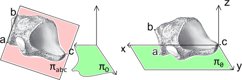
Averaging feature position and orientation. The illustration of the concept for averaging feature position and orientation, showed on cuboid example (bone drawings adapted from [60])
-
1.
-
Spherical harmonics (SPHARM) decomposition: The calculation of shape description is obtained by the SPHARM application [37–39].
-
Model and model order selection: To estimate the optimal model order for SPHARM decomposition, the Minimum Distance Length (MDL) criterion [40] was used. The product of SPHARM decomposition, i.e., the set of coefficients estimated in the SPHARM expansion characterises the shape of bone. For the SSM descriptive statistics of SPHARM coefficients were calculated.


Two-way parametric ANOVA was used to test for changes between tarsal bones in SPHARM coefficients [41]. This was followed by an application of a machine learning technique, the Random Forest [42], to the 4-class recognition problem of tarsal bones. For that, the total of 120 samples of either left or right tarsal bone models (15 individuals × 4 bones × 2 left/right) were used. 10-fold cross-validation method [43] was used to assess the misclassification error. Sensitivity and specificity for each classified group was also calculated.
Results
Figure 3 shows the box-plots for the first 25 SPHARM coefficients for left and right bones while Fig. 4 shows the first, second, and the third quartile as well as the mean of the 25 considered SPHARM coefficients. A 3D model of bones (see Fig. 5) is generated based on the mean estimate of coefficients for the right foot. Note that models shown in the figure are parted in order to exhibit the articular facets.

SPHARM estimates. The statistics of SPHARM estimates (box-plots) of the first 25 coefficients for the group of 15 left and 15 right models. Crosses indicate outliers

Descriptive statistics of SPHARM coefficients. The statistics of SPHARM estimates (the first, second, third quartile and mean) of the first 25 coefficients for the group of 15 left and 15 right models

Reconstruction of models. An example of reconstructed SSM of cuboid, navicular, talus and calcaneus for the right foot (blue - calcaneus, green - cuboid, magenta - navicular, cyan -talus)
Figure 6 presents the results of correlation between mean values of SPHARM coefficients for the right and left foot. The asymmetrical nature of bone can be assessed through examining the distribution of coefficients. The right/left foot correlation of estimated shapes is as follow: for cuboid (r 2=0.88), for navicular (r 2=0.99), for talus (r 2=0.98), for calcaneus (r 2=0.94), and statistically significant (p≪0.001) for all bones. Those correlations remain moderate when the highest coefficient is omitted, amounting to: for cuboid (r 2=0.72), for navicular (r 2=0.92), for talus (r 2=0.84), for calcaneus (r 2=0.54), and statistically significant (p≪0.001) for all bones (see Fig. 6 zoom).

Correlation between the SPHARM coefficients. Correlation between the SPHARM coefficients of the left and the right models of cuboid, navicular, talus and calcaneus
Two-way ANOVA showed statistically significant differences between considered bones, coefficients, and interactions between the bones and coefficients (all p≪0.001). Two tests were considered. One for all coefficients and the other one in which the third SPHARM coefficient was excluded (see Fig. 3), as it was substantially greater than the other coefficients and could influence the test. Nevertheless, similar statistically significant results (all p≪0.001) were obtained for the reduced set of SPHARM coefficients. The distribution of SPHARM coefficients was found to uniquely characterise each bone and so this distribution could be used for bone classification.
Further, the random forest algorithm was applied to develop a tarsal bone classifier. Considering data cross validation, the optimal number of decision trees was 40 and for that the misclassification rate was 1.02%. Sensitivity and specificity was estimated: for calcaneus 0.9600 and 0.9953, for cuboid 0.9960 and 0.9878, for navicular 1 and 0.9996, and for talus 0.9793 and 0.9958, respectively.
Discussion
Statistical shape modelling is a useful tool for feature extraction in medical imaging [12, 44]. The goal is to provide efficient information about the shape of an object of interest and its variability, often to build the so-called statistical atlas of particular body part, including bones [19, 45, 46]. Quantitative and accurate evaluation requires an appropriate representation used in shape modelling. The choice of the particular descriptors used in shape representation is important for further processing and analysis. The SPHARM description, used in this paper, provides quantitative information about the shape directly [47–49]. This paper contributes to this area by providing, for the first time, statistical anatomically accurate shape models for cuboid, navicular and talus.
Describing a shape using orthogonal polynomials, an inherent feature of SPHARM representation, allows for easy comparison of shapes through analysis of model coefficients. Further, it provides basis for classification of shapes based on testing for differences in the representative SPHARM coefficients. Using this methodology, our study shows that all considered tarsal bones can be uniquely represented by SPHARM.
Automated anatomical shape detection and classification have been considered in several applications of volumetric medical image analysis [32, 50–52]. Automated shape detection explores and applies the construction of algorithms that can learn from and make predictions on data. They are known as machine learning techniques and could assist in providing representative shape models as recently demonstrated by Cootes et al. [53], who used random forest regression voting for robust and accurate shape modelling. Among the many possible machine learning techniques we also employed the random forest algorithm but for the purpose of classification, which in our case showed high sensitivity and high specificity (both greater than 0.98) for all considered bones. The random forest technique is characterised by good accuracy for a relatively small number of samples (120 in our case) and containing a relatively high number of features (49 coefficients in the studied case). Also, it is robust to outliers in the input space and can rank the importance of variables considered in classification.
Another interesting aspect of statistical shape modelling is reconstruction [54–56]. The advantage of applying SPHARM to the shape reconstruction problem is their low complexity. Using estimated SPHARM coefficients it is possible to reconstruct one particular bone shape as well as create descriptive statistics for the examined group, say mean or median shape (see Fig. 5). It is worth noting that sexual dimorphism [57–59] was not considered in the study. The goal of the study was to develop anatomically accurate statistical models of tarsal bones and at that stage of research the size of bones was of concern. In other words, the statistical shape models of male bones are not necessarily scaled versions of their female equivalents.
Conclusions
Summarising, the SSMs of cuboid, navicular and talus created in this work correspond to anatomically accurate morphometric atlases (SSM which includes morphological characteristics and provides mathematical representation of the shape) that have not been previously considered. They extend the considerable amount of 3D SSMs that are already employed in medical imaging. The new models of the considered tarsal bones are of interest in medical image analysis, orthopaedics and biomechanics and could provide additional information for automated identification of pathologies, better diagnostics and treatment, preoperative planning, as well as for implant design and procedures.
References
Loncaric S. A survey of shape analysis techniques. Pattern Recogn. 1998; 31(8):983–1001.
Cootes TF, Taylor CJ, et al. Statistical models of appearance for computer vision. Technical report. Menchester: University of Manchester; 2004.
Cremers D, Rousson M, Deriche R. A review of statistical approaches to level set segmentation: integrating color, texture, motion and shape. Int J Comput Vision. 2007; 72(2):195–215.
Dryden IL, Mardia KV, Vol. 4. Statistical Shape Analysis. Chichester: John Wiley and Sons; 1998.
Bookstein FL. Morphometric Tools for Landmark Data: Geometry and Biology. Cambridge: Cambridge University Press; 1997.
O’Higgins P, Jones N. Facial growth in cercocebus torquatus: an application of three-dimensional geometric morphometric techniques to the study of morphological variation. J Anat. 1998; 193(2):251–72.
Fu G, Berg A, Das K, Li J, Li R, Wu R. A statistical model for mapping morphological shape. Theor Biol Med Model. 2010; 7(1):28.
Bruse JL, McLeod K, Biglino G, Ntsinjana HN, Capelli C, Hsia TY, Sermesant M, Pennec X, Taylor AM, Schievano S. A statistical shape modelling framework to extract 3d shape biomarkers from medical imaging data: assessing arch morphology of repaired coarctation of the aorta. BMC Med Imaging. 2016; 16(1):1.
Kendall DG, Barden D, Carne TK, Le H, Vol. 500. Shape and Shape Theory. Chichester: John Wiley & Sons; 2009.
Lele SR, Richtsmeier JT. An Invariant Approach to Statistical Analysis of Shapes. Boca Ralton, Florida: CRC Press; 2001.
Zhang D, Lu G. Review of shape representation and description techniques. Pattern Recogn. 2004; 37(1):1–19.
Heimann T, Meinzer HP. Statistical shape models for 3d medical image segmentation: a review. Med Image Anal. 2009; 13(4):543–63.
Pham DL, Xu C, Prince JL. Current methods in medical image segmentation 1. Annu Rev Biomed Eng. 2000; 2(1):315–37.
Peng B, Zhang L, Zhang D. A survey of graph theoretical approaches to image segmentation. Pattern Recogn. 2013; 46(3):1020–38.
Cootes TF, Taylor CJ, Cooper DH, Graham J. Active shape models-their training and application. Comput Vis Image Und. 1995; 61(1):38–59.
Lu YC, Untaroiu CD. Statistical shape analysis of clavicular cortical bone with applications to the development of mean and boundary shape models. Comput Meth Prog Bio. 2013; 111(3):613–28.
Berg AC, Berg TL, Malik J. Shape matching and object recognition using low distortion correspondences In: Schmid C, Soatto S, Tomasi C, editors. IEEE Computer Society Conference on Computer Vision and Pattern Recognition. USA: IEEE: 2005. p. 26–33.
Davies RH, Twining CJ, Cootes TF, Waterton JC, Taylor CJ. A minimum description length approach to statistical shape modeling. IEEE Trans Med Imaging. 2002; 21(5):525–37.
Seim H, Kainmueller D, Heller M, Lamecker H, Zachow S, Hege HC. Automatic Segmentation of the Pelvic Bones from CT Data Based on a Statistical Shape Model In: Botha CP, Kindlmann G, Niessen WJ, Preim B, editors. Eurographics Workshop on Visual Computing for Biomedicine. Netherlands: The Eurographics Association: 2008. p. 93–100.
Schmid J, Kim J, Magnenat-Thalmann N. Robust statistical shape models for mri bone segmentation in presence of small field of view. Med Image Anal. 2011; 15(1):155–68.
Kainmueller D, Lamecker H, Zachow S, Hege HC. An articulated statistical shape model for accurate hip joint segmentation In: Frangi A, editor. Engineering in Medicine and Biology Society, Annual International Conference of the IEEE. IEEE: 2009. p. 6345–351.
Yokota F, Okada T, Takao M, Sugano N, Tada Y, Tomiyama N, Sato Y. Automated ct segmentation of diseased hip using hierarchical and conditional statistical shape models. In: Medical Image Computing and Computer-Assisted Intervention. Berlin, Heidelberg: Springer: 2013. p. 190–7.
Stindel E, Udupa JK, Hirsch BE, Odhner D, Couture C. 3d mr image analysis of the morphology of the rear foot: application to classification of bones. Comput Med Imag Grap. 1999; 23(2):75–83.
Melinska AU, Romaszkiewicz P, Wagel J, Sasiadek M, Iskander DR. Statistical, morphometric, anatomical shape model (atlas) of calcaneus. PLOS ONE. 2015; 10(8):e0134603. Public Library of Science, doi:http://dx.doi.org/10.1371/journal.pone.0134603.
Chichka D, Stephenson J, Paulic A, Sheehan F. Bearing surface modeling of the talus and calcaneus. J Foot Ankle Res. 2008; 1(1):1.
Qiang M, Chen Y, Zhang K, Li H, Dai H. Measurement of three-dimensional morphological characteristics of the calcaneus using ct image post-processing. J Foot Ankle Res. 2014; 7(1):1.
Camacho DL, Ledoux WR, Rohr ES, Sangeorzan BJ, Ching RP. A three-dimensional, anatomically detailed foot model: a foundation for a finite element simulation and means of quantifying foot-bone position. J Rehabil Res Dev. 2002; 39(3):401–10.
Ledoux W, Camacho D, Ching R, Sangeorzan B. The development and validation of a computational foot and ankle model In: Enderle JD, editor. Engineering in Medicine and Biology Society, 2000. Proceedings of the 22nd Annual International Conference of the IEEE, vol. 4. USA: IEEE: 2000. p. 2899–902.
Liu J, Udupa JK, Saha PK, Odhner D, Hirsch BE, Siegler S, Simon S, Winkelstein BA. Rigid model-based 3d segmentation of the bones of joints in mr and ct images for motion analysis. Med Phys. 2008; 35(8):3637–49.
Leardini A, O’connor J, Catani F, Giannini S. A geometric model of the human ankle joint. J Biomech. 1999; 32(6):585–91.
Leardini A. Geometry and mechanics of the human ankle complex and ankle prosthesis design. Clin Biomech. 2001; 16(8):706–9.
Reggiani B, Leardini A, Corazza F, Taylor M. Finite element analysis of a total ankle replacement during the stance phase of gait. J Biomech. 2006; 39(8):1435–43.
Ito K, Hosoda K, Shimizu M, Ikemoto S, Kume S, Nagura T, Imanishi N, Aiso S, Jinzaki M, Ogihara N. Direct assessment of 3d foot bone kinematics using biplanar x-ray fluoroscopy and an automatic model registration method. J Foot Ankle Res. 2015; 8(1):21.
Pohle R, Toennies KD. Segmentation of medical images using adaptive region growing In: Sonka M, Hanson KM, editors. Medical Imaging 2001. San Diego, CA: International Society for Optics and Photonics: 2001. p. 1337–1346.
Kazhdan M, Hoppe H. Screened poisson surface reconstruction. ACM T Graphic (TOG). 2013; 32(3):29.
MeshLab. http://meshlab.sourceforge.net/, Accessed 5 Jan 2017.
Iskander DR. Modeling videokeratoscopic height data with spherical harmonics. Optom Vision Sci. 2009; 86(5):542–7.
Hobson EW. The theory of spherical and ellipsoidal harmonics. Cambridge: CUP Archive; 1931, pp. 40–82.
Vranić DV, Saupe D, Richter J. Tools for 3D-object retrieval: Karhunen-Loeve transform and spherical harmonics In: Dugelay JL, Rose K, editors. IEEE Fourth Workshop on Multimedia Signal Processing. IEEE: 2001. p. 293–8.
Rissanen J. Modeling by shortest data description. Automatica. 1978; 14(5):465–71.
Riffenburgh RH. Statistics in medicine. Amsterdam: Elsevier, Academic Press; 2012.
Breiman L. Random forests. Mach Learn. 2001; 45(1):5–32.
Mosteller F, Tukey JW. Data analysis, including statistics In: Jones LV, editor. The Collected Works of John W Tukey. Monterey, California: Wadswoorth & Brooks/Cole: 1968. p. 601–94.
Cootes TF, Taylor CJ. Anatomical statistical models and their role in feature extraction. Brit J Radiol. 2004; 77(2):133–39. British Institute of Radiology.
Chintalapani G, Ellingsen LM, Sadowsky O, Prince JL, Taylor RH. Statistical atlases of bone anatomy: construction, iterative improvement and validation In: Ayache N, Ourselin S, Maeder AJ, editors. Medical Image Computing and Computer-Assisted Intervention. Berlin Heidelberg: Springer: 2007. p. 499–506.
Dworzak J, Lamecker H, von Berg J, Klinder T, Lorenz C, Kainmüller D, Seim H, Hege HC, Zachow S. 3d reconstruction of the human rib cage from 2d projection images using a statistical shape model. Int J CARS. 2010; 5(2):111–24.
Styner MA, Rajamani KT, Nolte LP, Zsemlye G, Székely G, Taylor CJ, Davies RH. Evaluation of 3D correspondence methods for model building. In: Information processing in medical imaging. Berlin Heidelberg: Springer: 2003. p. 63–75.
Davies R, Taylor C, et al. Statistical models of shape: Optimisation and evaluation. London: Springer; 2008, pp. 9–45.
Davies RH, Twining CJ, Cootes TF, Taylor CJ. Building 3-d statistical shape models by direct optimization. IEEE T Med Imaging. 2010; 29(4):961–81.
Perperidis D, Mohiaddin R, Rueckert D. Construction of a 4D statistical atlas of the cardiac anatomy and its use in classification In: Duncan JS, Gerig G, editors. Medical Image Computing and Computer-Assisted Intervention. Berlin Heidelberg: Springer: 2005. p. 402–10.
Rodriguez A, Ehlenberger DB, Dickstein DL, Hof PR, Wearne SL. Automated three-dimensional detection and shape classification of dendritic spines from fluorescence microscopy images. PLOS ONE. 2008; 3(4):e1997. Public Library of Science, doi:http://dx.doi.org/10.1371/journal.pone.0001997.
Neubert A, Fripp J, Engstrom C, Schwarz R, Lauer L, Salvado O, Crozier S. Automated detection, 3d segmentation and analysis of high resolution spine mr images using statistical shape models. Phys Med Biol. 2012; 57(24):8357.
Cootes TF, Ionita MC, Lindner C, Sauer P. Robust and accurate shape model fitting using random forest regression voting In: Duncan JS, Gerig G, editors. Computer Vision-ECCV 2012. Berlin Heidelberg: Springer: 2012. p. 278–91.
Zheng G, Gollmer S, Schumann S, Dong X, Feilkas T, Ballester MAG. A 2d/3d correspondence building method for reconstruction of a patient-specific 3d bone surface model using point distribution models and calibrated x-ray images. Med Image Anal. 2009; 13(6):883–99.
Neubert A, Fripp J, Engstrom C, Schwarz D, Weber MA, Crozier S. Statistical shape model reconstruction with sparse anomalous deformations: Application to intervertebral disc herniation. Comput Med Imaging Graph. 2015; 46:11–9.
Zachow S, Lamecker H, Elsholtz B, Stiller M. Reconstruction of mandibular dysplasia using a statistical 3D shape model In: Schmidt DC, editor. International Congress Series, vol. 1281. Berlin: Elsevier: 2005. p. 1238–1243.
Bidmos MA, Dayal MR. Sex determination from the talus of south african whites by discriminant function analysis. Am J Foren Med Path. 2003; 24(4):322–8.
Bidmos MA, Asala SA. Sexual dimorphism of the calcaneus of south african blacks. J Forensic Sci. 2004; 49(3):JFS2003254–5.
Rosing FW, Graw M, Marre B, Ritz-Timme S, Rothschild MA, Rotzscher K, Schmeling A, Schroder I, Geserick G. Recommendations for the forensic diagnosis of sex and age from skeletons. HOMO-Journal of Comparative Human Biology. 2007; 58(1):75–89. Elsevier.
Gray H. Anatomy of the human body. Philadelphia: Lea & Febiger; 1918.
Acknowledgements
Authors would like to thank Aleksandra Habowska, Weronika Poszwa and Malgorzata Socha for gathering and preparing data for the analysis.
Funding
The research was supported by Polish National Centre of Science, under grant Preludium UMO-2013/09/N/ST7/03418.
Availability of data and materials
All data generated during this study are included in this published article. This is the full data set for coefficients for calcaneus, cuboid, navicular and talus. We attach text file containing Spherical Harmonics coefficients. Please contact us if you need more information how to prepare models using attached data. (Additional file 1).
Authors’ contributions
AM designed and carried out the experiments, analysed the data, and drafted the manuscript. PR gathered and prepared data to analysis, as well as validated models. JW gathered and prepared data to analysis, as well as validated models. BA analysed the data and drafted part of the manuscript. MS detailed research protocol to meet ethics approval and consent to participate as well as critically revised the manuscript and contributed to the evaluation part. DRI designed experiments and analysed the data as well as drafted the manuscript. All authors read and approved the final manuscript.
Competing interests
The authors declare that they have no competing interests.
Consent for publication
Not applicable.
Ethics approval and consent to participate
All subject records were anonymised and de-identified prior to processing according to the standard data release procedures. The Review Board of the Department of Radiology, Wroclaw Medical University, Wroclaw has approved the study. The study has been conducted according to the principles of the Declaration of Helsinki.
Author information
Authors and Affiliations
Corresponding author
Additional file
Additional file 1
SPHARM coefficients for calcaneus, cuboid, navicular and talus bones. (XLS 127 KB)
Rights and permissions
Open Access This article is distributed under the terms of the Creative Commons Attribution 4.0 International License(http://creativecommons.org/licenses/by/4.0/), which permits unrestricted use, distribution, and reproduction in any medium, provided you give appropriate credit to the original author(s) and the source, provide a link to the Creative Commons license, and indicate if changes were made. The Creative Commons Public Domain Dedication waiver(http://creativecommons.org/publicdomain/zero/1.0/) applies to the data made available in this article, unless otherwise stated.
About this article

Cite this article
Melinska, A.U., Romaszkiewicz, P., Wagel, J. et al. Statistical shape models of cuboid, navicular and talus bones. J Foot Ankle Res 10, 6 (2017). https://doi.org/10.1186/s13047-016-0178-x
Received:
Accepted:
Published:
DOI: https://doi.org/10.1186/s13047-016-0178-x