
Abstract
Background
The future of medicine is moving towards the phase of precision medicine, with the goal to prevent and treat diseases by taking inter-individual variability into account. A large part of the variability lies in our genetic makeup. With the fast paced improvement of high-throughput methods for genome sequencing, a tremendous amount of genetics data have already been generated. The next hurdle for precision medicine is to have sufficient computational tools for analyzing large sets of data. Genome-Wide Association Studies (GWAS) have been the primary method to assess the relationship between single nucleotide polymorphisms (SNPs) and disease traits. While GWAS is sufficient in finding individual SNPs with strong main effects, it does not capture potential interactions among multiple SNPs. In many traits, a large proportion of variation remain unexplained by using main effects alone, leaving the door open for exploring the role of genetic interactions. However, identifying genetic interactions in large-scale genomics data poses a challenge even for modern computing.
Results
For this study, we present a new algorithm, Grammatical Evolution Bayesian Network (GEBN) that utilizes Bayesian Networks to identify interactions in the data, and at the same time, uses an evolutionary algorithm to reduce the computational cost associated with network optimization. GEBN excelled in simulation studies where the data contained main effects and interaction effects. We also applied GEBN to a Type 2 diabetes (T2D) dataset obtained from the Marshfield Personalized Medicine Research Project (PMRP). We were able to identify genetic interactions for T2D cases and controls and use information from those interactions to classify T2D samples. We obtained an average testing area under the curve (AUC) of 86.8 %. We also identified several interacting genes such as INADL and LPP that are known to be associated with T2D.
Conclusions
Developing the computational tools to explore genetic associations beyond main effects remains a critically important challenge in human genetics. Methods, such as GEBN, demonstrate the utility of considering genetic interactions, as they likely explain some of the missing heritability.
Background
Over the past decade, development in large-scale, high-throughput methods to characterize the human genome has dramatically improved our ability to assess the relationship between an individuals’ genome and diseases [1]. With the ever-increasing generation of genomic data, development of computational methods necessary to analyze the vast amount of data are becoming increasingly important [2]. The genome-wide association study (GWAS) was the pioneering method to interrogate the genotypic and phenotypic relationship and is still being widely used today [3, 4]. However, despite GWAS’ wide success in finding associated SNPs in many common diseases, it lacks the power to detect more complex genetic architectures such as genetic interactions [5]. Therefore, a more comprehensive analysis method that can detect both main effects as well as genetic interactions is needed.
Much variability in human diseases and traits remain unexplained by using GWAS alone [5]. It is hypothesized that some of the missing variability could stem from complex genetic interactions that are unexplored by traditional association analysis. Furthermore, studies that do explore genetic interactions are often limited to two-way interactions due to the exponential increase of computational burden associated with higher-way interactions [6]. A number of analytic methods have been proposed and implemented to explore interactions using statistical and data mining strategies. For example, MDR [7, 8] can exhaustively evaluate all possible n-way interactions for a given n and selects the best model based on cross validations. Network based methods such as Neural Networks [9, 10] and Bayesian Networks [11] use their respective network structures to model interactions. Other notably machine learning methods including random forest [12] and SURF [13] use variable importance score to select potential interacting variables that are predictive of the outcome. However, strategies that employ exhaustive search are difficult to scale up due to the exponentially increasing search space. Machine learning methods are more flexible but they often suffer in model interpretability. Typically, the underlying pattern in data is not known a priori, thus it is important to develop a flexible method to model different types of genetic architecture.
To capture main effects of genetic variants as well as complex genetic interactions, we created the Grammatical Evolution Bayesian Network (GEBN) algorithm. The algorithm can simultaneously identify marginal effects as well as interaction effects without exponentially increasing the search time. GEBN can also identify interactions that occur between different sets of genetic variants in different groups (i.e. cases and controls). This flexibility allows discovery of non-overlapping genetic architectures in multiple groups. Previous Bayesian Networks methods to detect genetic interactions [11, 14] have been limited to a small set of input SNPs. Here, we specifically chose to implement an evolutionary computation strategy to evolve the structure of the Bayesian Network because it allows us to model a larger number of SNPs while controlling for the computational time.
We implemented GEBN algorithm in the software package ATHENA. We tested the algorithm on various simulation datasets. We also applied GEBN to a case–control dataset for type 2 diabetes obtained from the Marshfield Personalized Medicine Research Project Biobank (Marshfield PMRP) [15]. The network models identified novel interaction networks for type 2 diabetes cases and healthy individuals, respectively. Using the interaction networks for the two groups, we built prediction models that have an average AUC of 86 %. In the following sections, we describe the GEBN algorithm, data simulations and the application in type 2 diabetes. Our results demonstrate the promise of methods like GEBN.
Methods
Grammatical Evolution Bayesian Network (GEBN)
Bayesian Network is a multivariate modeling method that expresses the relationship of variables through a series of conditional distributions. The use of Bayesian Networks is becoming very important in biology because of their ability to infer biological networks [16], model signaling pathways [17], and classifications [18, 19]. The current obstacle for the application of Bayesian Networks in large-scale genomics data is the exponentially increase of search space with the increase of input variables. Thus, we used a grammatical evolution (GE) algorithm to evolve Bayesian Networks in order to reduce computational time. GE is a type of genetic programming [20, 21] that uses Backus-Naur Form (BNF) grammar to create a model based on a genetic algorithm. The advantage of GE algorithm lies in its guided random search so that the search space is greatly reduced. The steps of the GE algorithm is the following:
-
1.
Divide the data into five equal parts for cross-validations
For each cross validation:
-
2.
Populations of binary string are randomly generated and translated into functional Bayesian Networks by the grammar. For each individual genome, the binary string is divided into consecutive codons. The codons are then translated according to the grammar (Fig. 1).
Fig. 1 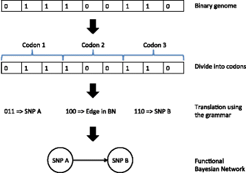
Generation of BN using the grammar
-
3.
Calculate the fitness of the Bayesian Networks using the K2 scoring function [22].
\( P\left({B}_s,D\right)=P\left({B}_s\right)\prod_{i=l}^n\prod_{j-1}^{q_i}\frac{r_i=1!}{\left({N}_{ij}+{r}_i-1\right)}{N}_{ij}\prod_{k=1}^{r_i}{N}_{ijk}! \)
Where D is the dataset, B is Bayesian Network, n is total number of variables, qi is the number of different values of Xi’s parents, ri is the number of values of Xi. The score calculates the probability of observing the network given the data.
-
4.
Select the Bayesian Networks that have the highest fitness, which will then undergo crossover and mutations. During crossover and mutation, parts of the different Bayesian Networks are exchanged or mutated to create new networks.
-
5.
Repeat 3–4 for a set number of generations
-
6.
Save the best model in the final generation and evaluate it on testing data

The final Bayesian Network is composed of connected and unconnected variables. Variables that are connected in the network are directly dependent with each other, while unconnected variables are conditionally independent. The advantage of GEBN over the more traditional network construction is that it can explore a wider search space, thus more suitable for large-scale genomics data. In addition, using an evolutionary search strategy removes the dependency on human trial and error to create optimal network structures and instead relies on the data and computation along with evolutionary learning to find optimal structures.
Discriminant analysis
The above GEBN method is applied to the case group and the control group independently. To prevent over-fitting, we used Bayesian Information Criteria (BIC) [23] to control the model complexity. The BIC is calculated as:
Where L is the maximum likelihood of data given a network, k is the number of free parameters, and n is the sample size. We iteratively removed each edge in the case or control network and calculated BIC for the reduced model. If the reduced model had higher BIC value, the edge was retained, and vice versa.
Finally, we used the discriminant analysis to assign an individual into either the case group or the control group. Using Bayes theorem, the probability of the sample belonging to a case group is calculated by:
Where \( P\left(Y= Case\right) \) and \( P\left(Y= Control\right) \) are given by their proportions in the total sample and \( P\left( Data\Big|Y= Case\right) \) is calculated as:
p = total number of variables. \( P\left( Data\Big|Y= Control\right) \) was calculated in the same fashion.
Genetic data simulation
To test our approach, we simulated data that contains functional SNP variables with main effects and interaction effects. For main effect simulation, we simulated data that consist of different numbers of functional SNPs with varying degrees of association to a binary outcome. For interaction effects, we separately simulated a number of interaction effects in case and control groups. We purposely made the interaction effects different in case and control groups to mimic different genetic architectures in two groups (Fig. 2).

Schematic of data simulation. Main effect models have different allele frequencies in case and control datasets at the simulated SNPs. In interaction effect models, cases and control datasets have different simulated interacting SNPs without main effects
To simulate different degrees of main effect, for a functional SNP, we altered the allele frequencies in the case data (Fcase) using a weighted average of allele frequencies in the control data (Fcontrol) and the extreme allele frequencies (Feffect) that were defined as (AA = 100 %, Aa = 0 %, aa = 0 %). Thus, the allele frequencies of the functional SNP in the case data is obtained by Fcase = w*Feffect + (1-w)*Fcontrol, where w is the weight index – larger w indicating more discrepancy between the case frequencies and control frequencies.
The interaction effects were simulated as follows: Let Find denotes the joint frequencies of a pair of uncorrelated SNPs, which is calculated as the product of marginal frequencies between SNPs. The correlation can be increased by relocating the frequencies from the off-diagonal to the diagonal in the frequency table, and an extreme case is that only the diagonal have non-zero frequencies, which is denoted by Fdiag. Different strength of interactions can be simulated by w*Fdiag + (1-w)* Find.
For each dataset, we used the simulated frequency tables with sampling with replacement to determine the genotype of the functional SNPs. Then, we embedded the functional SNPs into a dataset with random SNPs to make it comparable to real biological datasets. Details of simulation parameters are shown in Table 1.
Marshfield PMRP type 2 diabetes dataset
The Marshfield PMRP is a biobank that has collected ~20,000 adult subjects’ biological samples and electronic health records [15]. We obtained SNPs data of type 2 diabetes cases and controls who were genotyped on Illumina Human660W-Quad BeadChip. We only retained individuals who are European Americans because they account for over 95 % of samples and we also removed related samples. For SNP quality control (QC), we kept SNPs that have 100 % call rate and minor allele frequency > 5 %. The cleaned data consists of 267, 209 SNPs in 800 cases and 2465 controls. We then performed a GWAS using logistic regression to identify a set of candidate SNPs with main effects for GEBN analysis (this is a main effects filtering step [24]). Association analysis was performed while adjusting for sex, median BMI, and birth decade. Case–control status for T2D was determined using Mount Sinai’s diabetes algorithm [25] from the Diabetes HTN CKD algorithm [26].
Results and discussion
Simulation results
In the simulation study, we compared the performance of GEBN to that of the traditional GWAS approach based on logistic regression and another widely used method for detecting interactions, grammatical evolution neural network (GENN) [27, 28]. The prediction performance is summarized by the respective receiver operating characteristic (ROC) curves and the area under the curve (AUC). For each setting, we show the prediction performance averaged over 10 simulations. Regression models that include the exact simulated model (MAX) are also used to show the upper bound of prediction performance.
For main effect models, GEBN achieved close to maximum prediction performance in datasets with 100 SNPs. Logistic regression showed similar power, while GENN showed lower power. With 500 SNPs, the performance advantage of GEBN is even more visible (Fig. 3a-d). The performance of all methods were improved by increasing the number of functional SNPs and increasing the effect size.

Simulation results for additive and interaction models using grammatical evolution Bayesian Network (GEBN), grammatical evolution neural network (GENN), logistic regression, and logistic regression with the exact simulated model (MAX). The colors represent different weight indexes (red = 0.9, blue = 0.5, green = 0.1). These weight indices correspond to strength of the simulated effects. a. Main effect model: SNP A (100) b. Main effect model: SNP A (500) c. Main effect model: SNP A, B, C, D (100) d. Main effect model: SNP A, B, C, D (500) e. Interaction model: SNP A < − > B (100) f. Interaction: SNP A < − > B (500) g. Interaction model: SNP A < − > B, C < − > D, W < − > X, Y < − > Z (100) h. Interaction model: SNP A < − > B, C < − > D, W < − > X, Y < − > Z (500)
When case data and control data only differ by SNP interactions, logistic regression failed to separate two types with ROC curve fluctuating along the 45° line which corresponds to random guesses. GENN showed some power in detect interactions. However, GEBN showed improved ROC especially when the effect size is large (Fig. 3e-h). The execution time for GEBN depends on the parameter settings. With the current settings of population size of 3000 and 300 generations of evolution, the average running time is 1.5 ± 0.07 h for 100 SNPs and 0.97 ± 0.1 h for 500 SNPs and the running time is not dependent on the underlying model. The average AUC for all the models are listed in Table 2.
Type 2 diabetes results
We first performed association analysis using logistic regression for 267,209 SNPs associations with type 2 diabetes, using p < 0.001 as threshold, we identified 259 SNPs associated with type 2 diabetes. The top associated SNP was rs7903146 (p = 2.997e–06), which maps to TCF7L2 gene. To remove SNPs that are correlated, we used PLINK software [29] to prune the associated SNPs based on linkage disequilibrium (−−indep 50 5 2). 202 SNPs remained after LD pruning. We applied GEBN on the 202 SNPs, together with sex, median BMI, and birth decade, to separately build interaction networks for type 2 diabetes cases and controls. We then used the final network from cases and controls to perform discriminate analysis on the independent testing data. The average prediction AUC of 5-fold cross validation was 86.8 % (Fig. 4).

Testing ROC curve for type 2 diabetes. Each color represents a single cross-validation
Figure 5 shows the best Bayesian Network models for cases and controls. The AUC for the best model was 88.7 %. The networks also include the rest of the SNPs as marginal variables, but for clarity, they were not shown. The cases and controls share there common interactions: rs13127347 and rs2333452, rs9851100 and rs710563 (both in P3H2 gene), rs2666504 and rs1475563 (INADL gene). There was also one unique interaction for cases, which is rs10065876 and rs11741322 and two for controls, which are rs4477348 and rs6480213 (both in CTNNA3 gene), and rs11707430 and rs6444295 (both in LPP gene).

Best Bayesian Network models for cases and controls. Left panel shows network structure before BIC pruning. Right panel shows network structure after BIC pruning, and the red edges indicate interactions only found in the case data or the control data, but not both cases and controls. a. Case data network, b. Control data network
Conclusions
In this study, we presented a novel algorithm that can efficiently capture marginal and interaction effects present in the genetic data. We demonstrated in simulation data that GEBN performed equal or better than the standard GWAS analysis method using logistic regression as well as GENN on data with only main effect functional SNPs. In data with interacting SNPs, logistic regression failed to capture the true model which is shown by the ~50 % AUC (Fig. 2). GENN was able to capture simulated interactions, however, the predictive power were significantly lower than the MAX models, which gives the upper bound of prediction performance. On the other hand, GEBN were able to separately identify the unique interactions in cases and controls and use that information to distinguish the two groups. The performance of GEBN was close to the maximum prediction power in data with 100 and 500 SNPs. One concern was that GEBN can potentially over fit the data because networks were trained separately for each group. However, our testing AUCs showed that we did not over fit the model.
Using main effect filtering followed by GEBN analysis, we replicated canonical associations and also identified novel genetic interactions for type 2 diabetes. The most significant association was rs7903146, which is located in the TCF7L2 gene. We also identified rs12255372, which is in LD with rs7903146, as a significant association. TCF7L2 gene has been implicated for type 2 diabetes in many studies [30, 31]. We limited the network analysis to the top 202 associated SNPs because it is a comparable size to our simulation study. It is interesting that the top case and control networks have common as well as unique edges. The common edges include two non-coding SNPs on chromosome 4, two SNPs within P3H2 gene and one SNP in INADL gene and one SNP in the non-coding region of chromosome 1. The INADL gene is part of the hippo signaling pathway [32]. The pathway has been shown to regulate pancreas development [33] and adipocyte development [34]. Interestingly, a prior study has found that INADL was associated with children’s weight [35]. It is difficult to interpret the unique interaction for case group because both of the SNPs are located in non-coding regions. These could be further analyzed by looking into the ENCODE and GTEx regulatory data for possible functions. For controls, CTNNA3 were found to be associated with Alzheimer [36] and heart disease [37]. LPP gene has shown a robust association with type 2 diabetes in multiple ethnicities as well as combined meta-analysis [38]. Taken together, we have shown that GEBN have identified several known genes associated with type 2 diabetes. Using logistic regression, we also obtained a similar prediction AUC of 86.5 %. The similar performance was mostly due to the candidate SNPs were selected using a main effect filtering. Despite the similarity in the AUCs, GEBN was able to identify more complex genetic structures in diabetes cases and controls than logistic regression.
This paper presents the first step of the algorithm development that aims to address the pressing need for tools to identify complex relationships within the genetics data. Due to the flexibility of the Bayesian networks, the algorithm could be applied to datasets with more than two outcomes. For example, drug response phenotypes might be categorized as high responder, low responder, and non-responder. This would be possible to analyze with GEBN.
The utility of GEBN will be even greater in those settings because traditional statistical approaches are generally limited to binary outcomes. We also plan to integrate other –omics data such as transcriptomic and methylomic data into the network. The potential interactions between factors from different data types could reveal novel biological insights not seen at any individual data alone. The ultimate goal of individually identifying networks for different groups or subtypes of disease is to more precisely understand the disease so that we can improve detection and treatment of the disease. The method presented in this paper will help further elucidate the complex biological relationship present in the genetics data.
References
Mardis ER. Next-generation DNA sequencing methods. Annu Rev Genomics Hum Genet. 2008;9:387–402.
Ritchie MD, Holzinger ER, Li R, Pendergrass SA, Kim D. Methods of integrating data to uncover genotype–phenotype interactions. Nat Rev Genet. 2015;16(2):85–97.
Ritchie MD, Denny JC, Zuvich RL, Crawford DC, Schildcrout JS, Bastarache L, Ramirez AH, Mosley JD, Pulley JM, Basford MA, Bradford Y, Rasmussen LV, Pathak J, Chute CG, Kullo IJ, McCarty CA, Chisholm RL, Kho AN, Carlson CS, Larson EB, Jarvik GP, Sotoodehnia N, Manolio TA, Li R, Masys DR, Haines JL, Roden DM. Genome- and phenome-wide analyses of cardiac conduction identifies markers of arrhythmia risk. Circulation. 2013;127(13):1377–85.
Hindorff LA, Sethupathy P, Junkins HA, Ramos EM, Mehta JP, Collins FS, Manolio TA. Potential etiologic and functional implications of genome-wide association loci for human diseases and traits. Proc Natl Acad Sci U S A. 2009;106(23):9362–7.
Maher B. Personal genomes: the case of the missing heritability. Nature. 2008;456(7218):18–21.
Hall MA, Verma SS, Wallace J, Lucas A, Berg RL, Connolly J, Crawford DC, Crosslin DR, de Andrade M, Doheny KF, Haines JL, Harley JB, Jarvik GP, Kitchner T, Kuivaniemi H, Larson EB, Carrell DS, Tromp G, Vrabec TR, Pendergrass SA, McCarty CA, Ritchie MD. Biology-driven gene-gene interaction analysis of Age-related cataract in the eMERGE network. Genet Epidemiol. 2015;39(5):376–84.
Ritchie MD, Hahn LW, Roodi N, Bailey LR, Dupont WD, Parl FF, Moore JH. Multifactor-dimensionality reduction reveals high-order interactions among estrogen-metabolism genes in sporadic breast cancer. Am J Hum Genet. 2001;69(1):138–47.
Hahn LW, Ritchie MD, Moore JH. Multifactor dimensionality reduction software for detecting gene-gene and gene-environment interactions. Bioinformatics. 2003;19(3):376–82.
Holzinger ER, Dudek SM, Frase AT, Pendergrass SA, Ritchie MD. ATHENA: the analysis tool for heritable and environmental network associations. Bioinformatics. 2013;30:1–9.
Beam AL, Motsinger-Reif A, Doyle J. Bayesian neural networks for detecting epistasis in genetic association studies. BMC Bioinformatics. 2014;15(1):368.
Jiang X, Barmada MM, Visweswaran S. Identifying genetic interactions in genome-wide data using Bayesian networks. Genet Epidemiol. 2010;34(6):575–81.
Winham SJ, Colby CL, Freimuth RR, Wang X, de Andrade M, Huebner M, Biernacka JM. SNP interaction detection with random forests in high-dimensional genetic data. BMC Bioinformatics. 2012;13(1):164.
Greene CS, Penrod NM, Kiralis J, Moore JH. Spatially uniform relieff (SURF) for computationally-efficient filtering of gene-gene interactions. BioData Min. 2009;2(1):5.
Han B, Park M, Chen X. A Markov blanket-based method for detecting causal SNPs in GWAS. BMC Bioinformatics. 2010;11(3):S5.
McCarty CA, Wilke RA, Giampietro PF, Wesbrook SD, Caldwell MD. Marshfield clinic Personalized Medicine Research Project (PMRP): design, methods and recruitment for a large population-based biobank. Per Med. 2005;2(1):49–79.
Friedman N. Inferring cellular networks using probabilistic graphical models. Science. 2004;303(5659):799–805.
Sachs K, Perez O, Pe’er D, Lauffenburger DA, Nolan GP. Causal protein-signaling networks derived from multiparameter single-cell data. Science. 2005;308(5721):523–9.
Bradford JR, Needham CJ, Bulpitt AJ, Westhead DR. Insights into protein-protein interfaces using a Bayesian network prediction method. J Mol Biol. 2006;362(2):365–86.
Cooper GF, Hennings-yeomans P, Visweswaran S, Barmada M. An efficient bayesian method for predicting. Clinical Outcomes from Genome-Wide Data. 2010;13:127–31.
O’Neill M, Ryan C. Grammatical Evolution: Evolutionary Automatic Programming in an Arbitrary Language. Springer; 2003 edition, 2003.
O’Neill M, Ryan C. Grammatical evolution. IEEE Trans Evol Comput. 2001;5(4):349–58.
Cooper GF, Herskovits E. A Bayesian method for the induction of probabilistic networks from data. Mach Learn. 1992;9(4):309–47.
Schwarz G. Estimating the dimension of a model. Ann Stat. 1978;6(2):461–4.
Sun X, Lu Q, Mukherjee S, Mukheerjee S, Crane PK, Elston R, Ritchie MD. Analysis pipeline for the epistasis search - statistical versus biological filtering. Front Genet. 2014;5:106.
Kho AN, Hayes MG, Rasmussen-Torvik L, Pacheco JA, Thompson WK, Armstrong LL, Denny JC, Peissig PL, Miller AW, Wei W-Q, Bielinski SJ, Chute CG, Leibson CL, Jarvik GP, Crosslin DR, Carlson CS, Newton KM, Wolf WA, Chisholm RL, Lowe WL. Use of diverse electronic medical record systems to identify genetic risk for type 2 diabetes within a genome-wide association study. J Am Med Inform Assoc. 2012;19(2):212–8.
Nadkarni GN, Gottesman O, Linneman JG, Chase H, Berg RL, Farouk S, Nadukuru R, Lotay V, Ellis S, Hripcsak G, Peissig P, Weng C, Bottinger EP. Development and validation of an electronic phenotyping algorithm for chronic kidney disease. AMIA Annu Symp Proc. 2014;2014:907–16.
Holzinger ER, Dudek SM, Frase AT, Krauss RM, Medina MW, Ritchie MD. ATHENA: a tool for meta-dimensional analysis applied to genotypes and gene expression data to predict HDL cholesterol levels. Pac Symp Biocomput. 2013:385–96.
Holzinger ER, Dudek SM, Frase AT, Pendergrass SA, Ritchie MD. ATHENA: the analysis tool for heritable and environmental network associations. Bioinformatics. 2014;30(5):698–705.
Purcell S, Neale B, Todd-Brown K, Thomas L, Ferreira MAR, Bender D, Maller J, Sklar P, de Bakker PIW, Daly MJ, Sham PC. PLINK: a tool set for whole-genome association and population-based linkage analyses. Am J Hum Genet. 2007;81(3):559–75.
Chandak GR, Janipalli CS, Bhaskar S, Kulkarni SR, Mohankrishna P, Hattersley AT, Frayling TM, Yajnik CS. Common variants in the TCF7L2 gene are strongly associated with type 2 diabetes mellitus in the Indian population. Diabetologia. 2007;50(1):63–7.
Gloyn AL, Braun M, Rorsman P. Type 2 diabetes susceptibility gene TCF7L2 and its role in beta-cell function. Diabetes. 2009;58(4):800–2.
Kanehisa M, Goto S. KEGG: kyoto encyclopedia of genes and genomes. Nucleic Acids Res. 2000;28(1):27–30.
George NM, Day CE, Boerner BP, Johnson RL, Sarvetnick NE. Hippo signaling regulates pancreas development through inactivation of Yap. Mol Cell Biol. 2012;32(24):5116–28.
An Y, Kang Q, Zhao Y, Hu X, Li N. Lats2 modulates adipocyte proliferation and differentiation via hippo signaling. PLoS One. 2013;8(8):e72042.
Comuzzie AG, Cole SA, Laston SL, Voruganti VS, Haack K, Gibbs RA, Butte NF. Novel genetic loci identified for the pathophysiology of childhood obesity in the Hispanic population. PLoS One. 2012;7(12):e51954.
Miyashita A, Arai H, Asada T, Imagawa M, Matsubara E, Shoji M, Higuchi S, Urakami K, Kakita A, Takahashi H, Toyabe S, Akazawa K, Kanazawa I, Ihara Y, Kuwano R. Genetic association of CTNNA3 with late-onset Alzheimer’s disease in females. Hum Mol Genet. 2007;16(23):2854–69.
van Hengel J, Calore M, Bauce B, Dazzo E, Mazzotti E, De Bortoli M, Lorenzon A, Li Mura IEA, Beffagna G, Rigato I, Vleeschouwers M, Tyberghein K, Hulpiau P, van Hamme E, Zaglia T, Corrado D, Basso C, Thiene G, Daliento L, Nava A, van Roy F, Rampazzo A. Mutations in the area composita protein αT-catenin are associated with arrhythmogenic right ventricular cardiomyopathy. Eur Heart J. 2013;34(3):201–10.
Mahajan A, Go MJ, Zhang W, Below JE, Gaulton KJ, Ferreira T, Horikoshi M, Johnson AD, Ng MCY, Prokopenko I, Saleheen D, Wang X, Zeggini E, Abecasis GR, Adair LS, Almgren P, Atalay M, Aung T, Baldassarre D, Balkau B, Bao Y, Barnett AH, Barroso I, Basit A, Been LF, Beilby J, Bell GI, Benediktsson R, Bergman RN, Boehm BO, Boerwinkle E, Bonnycastle LL, Burtt N, Cai Q, Campbell H, Carey J, Cauchi S, Caulfield M, Chan JCN, Chang L-C, Chang T-J, Chang Y-C, Charpentier G, Chen C-H, Chen H, Chen Y-T, Chia K-S, Chidambaram M, Chines PS, Cho NH, Cho YM, Chuang L-M, Collins FS, Cornelis MC, Couper DJ, Crenshaw AT, van Dam RM, Danesh J, Das D, de Faire U, Dedoussis G, Deloukas P, Dimas AS, Dina C, Doney AS, Donnelly PJ, Dorkhan M, van Duijn C, Dupuis J, Edkins S, Elliott P, Emilsson V, Erbel R, Eriksson JG, Escobedo J, Esko T, Eury E, Florez JC, Fontanillas P, Forouhi NG, Forsen T, Fox C, Fraser RM, Frayling TM, Froguel P, Frossard P, Gao Y, Gertow K, Gieger C, Gigante B, Grallert H, Grant GB, Grrop LC, Groves CJ, Grundberg E, Guiducci C, Hamsten A, Han B-G, Hara K, Hassanali N, Hattersley AT, Hayward C, Hedman AK, Herder C, Hofman A, Holmen OL, Hovingh K, Hreidarsson AB, Hu C, Hu FB, Hui J, Humphries SE, Hunt SE, Hunter DJ, Hveem K, Hydrie ZI, Ikegami H, Illig T, Ingelsson E, Islam M, Isomaa B, Jackson AU, Jafar T, James A, Jia W, Jöckel K-H, Jonsson A, Jowett JBM, Kadowaki T, Kang HM, Kanoni S, Kao WHL, Kathiresan S, Kato N, Katulanda P, Keinanen-Kiukaanniemi KM, Kelly AM, Khan H, Khaw K-T, Khor C-C, Kim H-L, Kim S, Kim YJ, Kinnunen L, Klopp N, Kong A, Korpi-Hyövälti E, Kowlessur S, Kraft P, Kravic J, Kristensen MM, Krithika S, Kumar A, Kumate J, Kuusisto J, Kwak SH, Laakso M, Lagou V, Lakka TA, Langenberg C, Langford C, Lawrence R, Leander K, Lee J-M, Lee NR, Li M, Li X, Li Y, Liang J, Liju S, Lim W-Y, Lind L, Lindgren CM, Lindholm E, Liu C-T, Liu JJ, Lobbens S, Long J, Loos RJF, Lu W, Luan J, Lyssenko V, Ma RCW, Maeda S, Mägi R, Männisto S, Matthews DR, Meigs JB, Melander O, Metspalu A, Meyer J, Mirza G, Mihailov E, Moebus S, Mohan V, Mohlke KL, Morris AD, Mühleisen TW, Müller-Nurasyid M, Musk B, Nakamura J, Nakashima E, Navarro P, Ng P-K, Nica AC, Nilsson PM, Njølstad I, Nöthen MM, Ohnaka K, Ong TH, Owen KR, Palmer CNA, Pankow JS, Park KS, Parkin M, Pechlivanis S, Pedersen NL, Peltonen L, Perry JRB, Peters A, Pinidiyapathirage JM, Platou CG, Potter S, Price JF, Qi L, Radha V, Rallidis L, Rasheed A, Rathman W, Rauramaa R, Raychaudhuri S, Rayner NW, Rees SD, Rehnberg E, Ripatti S, Robertson N, Roden M, Rossin EJ, Rudan I, Rybin D, Saaristo TE, Salomaa V, Saltevo J, Samuel M, Sanghera DK, Saramies J, Scott J, Scott LJ, Scott RA, Segrè AV, Sehmi J, Sennblad B, Shah N, Shah S, Shera AS, Shu XO, Shuldiner AR, Sigurđsson G, Sijbrands E, Silveira A, Sim X, Sivapalaratnam S, Small KS, So WY, Stančáková A, Stefansson K, Steinbach G, Steinthorsdottir V, Stirrups K, Strawbridge RJ, Stringham HM, Sun Q, Suo C, Syvänen A-C, Takayanagi R, Takeuchi F, Tay WT, Teslovich TM, Thorand B, Thorleifsson G, Thorsteinsdottir U, Tikkanen E, Trakalo J, Tremoli E, Trip MD, Tsai FJ, Tuomi T, Tuomilehto J, Uitterlinden AG, Valladares-Salgado A, Vedantam S, Veglia F, Voight BF, Wang C, Wareham NJ, Wennauer R, Wickremasinghe AR, Wilsgaard T, Wilson JF, Wiltshire S, Winckler W, Wong TY, Wood AR, Wu J-Y, Wu Y, Yamamoto K, Yamauchi T, Yang M, Yengo L, Yokota M, Young R, Zabaneh D, Zhang F, Zhang R, Zheng W, Zimmet PZ, Altshuler D, Bowden DW, Cho YS, Cox NJ, Cruz M, Hanis CL, Kooner J, Lee J-Y, Seielstad M, Teo YY, Boehnke M, Parra EJ, Chambers JC, Tai ES, McCarthy MI, Morris AP, 2014. Genome-wide trans-ancestry meta-analysis provides insight into the genetic architecture of type 2 diabetes susceptibility. Nat Genet 46(3), 234–44.
Acknowledgement
This work was supported by the NSF graduate fellowship (DGE1255832). Any opinions, findings, and conclusions or recommendations expressed in this material are those of the author(s) and do not necessarily reflect the views of the National Science Foundation.
Funds were also contributed by NIH grants HG006389, P50GM115318 and F31 HG008588.
Author information
Authors and Affiliations
Corresponding authors
Additional information
Competing interests
The authors declare that they have no competing interests.
Authors’ contributions
RL conceived the problem, developed the solution, analyzed the data, and led the drafting of the manuscript. SD implemented the GEBN algorithm. DK helped developed the solution. MA and YB helped preparing the data. PP, MB, JL, and CM provided the SNP data and provided revisions. LB developed the solution, designed the study, and helped the drafting of the manuscript. MR conceived the problem, designed the study, and revised the manuscript. All authors read and approved the final manuscript.
Rights and permissions
Open Access This article is distributed under the terms of the Creative Commons Attribution 4.0 International License (http://creativecommons.org/licenses/by/4.0/), which permits unrestricted use, distribution, and reproduction in any medium, provided you give appropriate credit to the original author(s) and the source, provide a link to the Creative Commons license, and indicate if changes were made. The Creative Commons Public Domain Dedication waiver (http://creativecommons.org/publicdomain/zero/1.0/) applies to the data made available in this article, unless otherwise stated.
About this article

Cite this article
Li, R., Dudek, S.M., Kim, D. et al. Identification of genetic interaction networks via an evolutionary algorithm evolved Bayesian network. BioData Mining 9, 18 (2016). https://doi.org/10.1186/s13040-016-0094-4
Received:
Accepted:
Published:
DOI: https://doi.org/10.1186/s13040-016-0094-4