
Abstract
Modern urban-transport planning requires evidence-based insights into current transport flows to better understand the needs and impacts of policymaking. Urban transport includes passenger and freight vehicles, which have different behavior, and the need for such a separation is often ignored in research and practice [1]. New digital data sources provide an opportunity to better understand urban transport and identify where policy interventions are required. We review the literature on digital counting techniques to monitor transport flows, including loops, Automatic-Number Plate Recognition (ANPR) cameras and floating car data. We further investigate the potential of ANPR cameras, which are widely deployed, and which can be augmented with vehicle category information. This article presents the methodology that we follow for transforming raw augmented ANPR camera data into practical knowledge for city planners. Our is aim is to provide a better understanding of passenger and freight vehicle movements and stops, identifying similarities and differences between vehicle categories. We demonstrate our methodology on a case study for the Mechelen-Willebroek district in Belgium, encompassing augmented data from 122 ANPR cameras for a period of two weeks. Additionally, we also look at the car-reduced zone and how time restrictions affect the different vehicle categories’ actions. The findings are validated with GPS data from heavy-good vehicles in the same period. The potential of augmented ANPR camera data and promising themes and applications of this data source are illustrated through the case study.
1 Introduction
Information and communication technologies (ICTs) have been transforming traditional methods of urban management and infrastructure planning for the past two decades [2]. In order to manage daily operations, urban-policy makers are increasingly using real-time analytics [2], for example, analyzing movement of vehicles in cities in order to monitor traffic and adjust traffic lights and speed limits [3].
In a complex environment such as the urban transportation, understanding travel behavior is a critical requirement of any attempt to foresee the impacts of change and to respond through policy. Several techniques can be used to collect urban transport data: traffic counts (loops or manual counts), vehicle observations, stakeholder surveys, driver interviews, vehicle trip diaries, Floating-Car Data (FCD), etc. [4–7]. Data from ANPR cameras has already been analyzed for traffic management, to estimate travel time and to understand vehicles travel behavior. A more detailed discussion on literature analyzing ANPR cameras data is provided in Section 2. In this research, we add to the state-of-the-art by focusing on analyzing augmented ANPR camera data to analyze different vehicle categories, i.e light-goods vehicles, heavy-goods vehicles and passenger vehicles, separately, and understand similarity and differences among these categories. Although increasingly called for, not many studies to date use a data source to compare different vehicle categories movement. Furthermore, we provide a comprehensive view on potentials of ANPR camera data in providing insights on movements of vehicles in a region, while most research concentrate on one aspect of transport. We guide ourselves by extracting knowledge for city planners that is relevant but missing. We provide visualizations on locations where vehicles have visited more frequently, and their frequent trajectories. Moreover, we demonstrate the number of vehicles during different hours of the day. Finally, we also focus on detecting stops (often called stay-point [8]) using ANPR cameras data, and we identify the location of the stops as well.
Many of the data sources do not differentiate vehicle categories and measure the flows of all vehicles at once. Manual counting and doing surveys can differentiate between vehicle categories, but this is cost and time intensive. Using technology to collect data can overcome the challenges of data collection, by providing large quantities of urban data at a much lower cost than traditional surveys [4, 5]. Data from induction loops can separate different vehicle categories [9], but detailed flows can not be derived as vehicles can not be easily tracked from one counting loop to the other. On the other hand, GPS data are typically collected within a single vehicle category, e.g. taxis [10–13], public transport vehicles [14, 15], passenger cars [16–19] (e.g. as part of an insurance or fleet plan) or freight vehicles [20–23].
What is missing are data sources that can measure both and separate passenger and freight flows. Passenger vehicles are the majority of observations, and freight vehicles count for 10 to 18% of all vehicles on urban roads [1]. On the other hand, these vehicles are responsible for 16% to 50% of transport-related emission of air pollutants in cities (depending on the pollutant considered) [1, 24]. Passenger and freight vehicles have different behavior, and it is essential to separate them to establish policies for each category accordingly.
Collecting data on urban-goods movement is specifically challenging as there are many economic agents who are reluctant to share information on their operations [25]. Yet decision makers need a solid understanding of patterns in urban freight operations and advanced forecasting tools to come to effective policies [26–28]. And ideally, this would include data from both freight and passenger flows, such that the effect of one on the other can be taken into account.
In this study we take a deeper look at data generated by Automatic Number Plate Recognition (ANPR) cameras, and their advantage for urban authorities to understand urban transport in their city. From a practical point of view, using data from ANPR cameras reduces cost and data ownership issues. First, because the cameras are mainly used for law enforcement purposes and electronic toll collections, there is often a dense network of cameras. Moreover, unlike loops, the cameras are installed for a specific purpose, and their use for transport monitoring requires no additional investment. Second, the cameras are often owned by authorities, or operated on their behalf, which gives them access to the data and overcomes ownership issues and costs linked to buying data from private operators (e.g. FCD data). The objective of the present paper is to demonstrate how ANPR camera data can contribute to a better contextual understanding of urban transport, by investigating movement of passenger vehicles and freight vehicles.
For the specific challenge of differentiating passenger and freight vehicles, we assume the possibility to augment the data with vehicle category information, e.g. by matching the number plates to “Vehicle Registration Service” records. This provides the opportunity to group the vehicles into different categories, e.g. passenger vehicles, light-goods vehicles and heavy-goods vehicles [29, 30]. We adapt a methodology for analysing such data, based on the generic CRISP-DM framework [31].
We provide a case study of the analysis of such a data source, with augmented ANPR camera data for the police district of Mechelen-Willebroek in Belgium. There are 122 ANPR cameras in this police district of 92,6 square kilometres1. Moreover, Mechelen-Willebroek district has recently implemented a car-reduced zone of 0.27 square kilometres. We analyze vehicles movements in this zone, to understand the effect of such policies in the region. The dataset was anonymized by the “Belgian Vehicle Registration Service”, removing the number plates but adding further information on the vehicles categories. In order to validate the results from the ANPR analysis, we have analyzed data from On-Board Units (OBU) of Heavy-Goods Vehicles (HGVs) and compared our findings from the two dataset.
In this research we start by reviewing the use of data from ANPR cameras and other sensors for understanding urban transport flows in Section 2. Afterwards, in Section 3, we describe our methodology, inspired by CRISP-DM [31], for processing and analyzing ANPR camera data to observe passenger and freight vehicles movements. In Section 4, in a case study we analyze augmented ANPR camera data, for the Mechelen-Willebroek police district. By exploring the methodology’s outputs, we describe the observed similarities and differences between different vehicle categories. Furthermore, we monitor the effect of the introduced car-reduced zone of the city of Mechelen in vehicles movements. Finally, in Section 5, we validate results from the ANPR analysis by analyzing GPS data from on-board units of HGVs. We investigate the observed similarity and differences. The paper is finalized by a conclusion in Section 6, and a discussion on limitations and future work in Section 7.
2 Literature review
Inductive loops, Bluetooth detectors, Floating Car Data (FCD), and ANPR cameras are the most common data sources that provide information on location of vehicles in real-time. In the following, we highlight the use of these digital data sources with a special focus on the latter.
Inductive loop traffic detectors Inductive loops are devices which are installed under the pavement to detect when a vehicle passes over it, while roughly classifying what category of vehicle it is [32]. They can hence be used to measure lane occupancy and volume of traffic at a certain point. Furthermore, two consecutive detectors can be placed with some distance apart to estimate average speed [33, 34].
Loops can be used for travel time estimation as they record velocities of vehicles at each point [35–37]. Furthermore, [38] proposes a single loop system that enables monitoring truck volume data based on weight of the truck. By comparing GPS and loop detectors data for estimating velocity and travel times, [39, 40] find out that using each data set alone gives an error rate of below 10% and combing both is better. Furthermore, [41] compare two techniques for predicting traffic state by estimating vehicles velocities using GPS data and loops detectors.
Bluetooth recognition systems Such a system records unique MAC-Addresses (Media-Access-Control-Address) of devices that pass it, e.g. from the smartphone of a driver, or the hands-free sets of a vehicle [42].
[42] survey the evolution and application of these systems. For example, they have been used to estimate travel time [43, 44]. [45] use GPS data from buses and Bluetooth detectors data for other vehicles and studies the travel patterns, and detects communities based on these patterns. [46] studies route choice modeling of vehicles, even though he reports that 30% of node sequences are effected by errors of the road side Bluetooth systems. Bluetooth recognition systems have lower detection rates than loops and ANPR cameras because not every vehicle has a bluetooth device, furthermore, the category of vehicle can not be derived from it.
Floating-Car Data (FCD) Locating vehicles in real time is the principle of floating-car data [47]. There are two main types of FCD, namely GPS and cellular-based systems. Global Positioning System (GPS), or more generally a Global Navigation Satellite System (GNSS) is a navigation system that provides geo-spatial information to any GPS receiver, e.g. a mobile phone or a vehicle’s navigation system. When locations of the receiver of a vehicle are stored at a certain interval, a trajectory of the vehicle is obtained. Because the receiver is on the driving vehicle, it is a form of FCD. In cellular-based system a mobile phone’s position is transmitted to the network [47]. This approach provides a high coverage as the mobile phones need to be turned on, but not necessarily in use.
Clearly, databases of GPS trajectories are a rich data source for analyzing transport behavior of vehicles. Alike other mentioned data sources, GPS data have been used for travel time estimation [48–51]. Other performance measures such as duration, distances, number of activities and origin-destination have been investigated using GPS trajectories data [20–23].
Additionally, in order to understand travel behavior in vehicles and humans, [16, 17, 52] group users into behavioral categories based on their travel patterns, and researchers in [53, 54] derive mobility measures and profiles for the users. While analyzing GPS trajectories data of freight vehicles, [55–57] discuss their method and challenges for identifying a stop.
Based on cellular-phone data, [58] measures traffic speeds and travel times, and compares those with findings from dual loop detectors. [59] also investigates vehicles velocities. Trip distributions and densities are studied by [60] and [61]. Finally, researchers in [62, 63] estimate travel demands in the form of origin-destination (OD) matrices.
Automatic Number (or License) Plate Recognition cameras These camera’s are installed in fixed locations and can read a vehicle’s registration plate with high accuracy. Recognizing the number plates is a difficult as factors such as illumination conditions, vehicle shadow and non-uniform size of license plate characters, different font and background color affect the performance of ANPR. This makes it hard to achieve 100% overall accuracy [64, 65]. ANPR cameras are widely employed around the world, mainly for law enforcement purposes and electronic toll collections. [66] report on use of ANPR cameras in London, Melbourne, Sydney and Seattle, which are among the smartest cities according to their bench marking. Governments do not always report on the number of cameras that have been installed, but records show that in the Netherlands close to 300 ANPR cameras have been installed [67], and in Denmark 24 at fixed locations and 48 on police cars [68]. In Australia and Belgium more than 1000 cameras have been installed [69, 70], and in Belgium this number is rising to three times more [70].
We review different uses of ANPR camera that have been studied:
Travel time Travel time on roads is a common indicator that can be estimated from the data received from these cameras [71–73], furthermore the effect of events on travel time can also be determined [74, 75]. In order to filter out the travel time errors, [76] use the “overtaking” method, which compares the travel time to the travel time of consecutive vehicles. In a further step, [77] have combined the estimated travel time with historic data to predict travel time in near future, and [78] propose to use ANPR camera data for predicting arrival time of trucks to their freight centers. [79] compare travel time estimation using ANPR camera data and GPS data, and do not detect any statistical differences. Moreover, in [5, 80] Hargrove compares different data sources for travel time estimation, using ANPR as the ground truth. [81] investigate travel time and traffic volume using ANPR camera data. Furthermore, vehicles are classified based on their emission standard, and finally their origin and destination is predicted based on origin of their number plate [81].
Traffic management In order to further plan traffic-management actions, [82] study effectiveness of a recently installed traffic management system which has boards for conveying messages, using ANPR in combination with weather data. In London [75], data from ANPR and CCTV cameras are used to understand the traffic composition of different vehicle groups based on number of vehicles and kilometers. Furthermore, they investigated the average speed, and the effect of events on that. Furthermore, [83] estimate speed profile and emission of vehicle, and [84] propose a model for real-time queue length calculations on freeways.
Origin-Destination [85] provide counts at each camera point and a matrix of origin-destination between camera pairs, that were the first and last camera observing a vehicle. [86] estimate the path flows and origin-destination. Thereafter, in [87] they optimize the use of ANPR cameras by minimizing the number of cameras needed for path estimation. Furthermore, [88] propose a trajectory reconstruction method based on ANPR camera data.
Travel behavior Matching the number plates with some socioeconomic factors of vehicle owners, [89] investigate effect of household size and household median income, on transport behavior of vehicles. [90] study the potential of carpooling using the traffic demand estimated from ANPR camera data. Furthermore, [91] explore regularity of arrival times in different individual vehicles. Researchers in [92–95] investigate activity patterns of vehicles based on their spatio-temporal features.
Cameras other than ANPR cameras have also been used to get an insight into transport. [96] estimate travel time from surveillance cameras and [4] review current applications of video and image processing cameras for ITS. There have been concerns about privacy regarding the use of cameras and the potential for mass surveillance. [97] investigate privacy risks and best practices of ANPR camera data use. Succeeding the establishment of a platform that respects the privacy of individuals, ANPR camera data can provide useful insights into urban transport.
We contribute to both literature and practice in two ways. First, as opposed to current research that has mostly concentrated on one aspect of transport e.g. travel time or origin-destination, we offer a more holistic and comprehensive approach on the potential of ANPR camera data. We investigate what performance measures can be derived from ANPR camera data for better understanding of vehicles movements. Thereafter, we propose a generic step-by-step approach to analyze ANPR data and derive these performance measures. We also showcase our methodology and discuss our findings on a few weeks’ data. For example, we investigate the vehicles movements in the region by looking into observation pairs, and we do not only look at vehicle movements but also at stops, e.g. where and how frequently vehicles stops. Second, using augmented ANPR camera data we explicitly differentiate between vehicle categories, i.e light-goods vehicles, heavy-goods vehicles and passenger vehicles, and accentuate differences among these categories. Although increasingly called for, no study to date has reported on a similar endeavor.
3 Methodology
To analyze the data, we follow a methodology that is inspired by CRISP-DM (CRoss-Industry Standard Process for Data Mining) [31]. CRISP-DM is a standard process that describes the different stages in a data analytics approach. These stages are “1. Business Understanding” where the business objectives are identified, “2. Data Understanding” where the data are described and explored, “3. Data Preparation” where data are selected, cleaned, and constructed, “4. Data Modeling” where the actual analysis is carried out and “5. Evaluation” where the results are interpreted, and finally “6. Deployment” where the process is operationalised.
We map these different stages to the analysis of raw augmented ANPR camera data to get insights into urban transport. This is non-trivial, as ANPR camera data are raw and noisy big data, which must be carefully treated and analysed before conclusions can be drawn from it. Figure 1 shows the different stages, which map to the CRISP-DM stages, and the kinds of data transformations that are applied in each. In the following, the steps are described in more details, highlighting our approach in this study.

Our methodology for analyzing observations of ANPR cameras
3.1 Business understanding: understanding urban transport
Concrete and up-to-date numbers on urban transport are often lacking for decision makers. The aim of this analysis is to analyze raw ANPR camera data, and provide insights into movement of different vehicle categories, e.g. passenger, light-goods and heavy-goods vehicles. The number of vehicles, common locations, entry-exit behavior, stopping locations and trajectories of different vehicle categories can be compared to each other. This should lead to a better understanding of urban transport and hence to better and more informed decision making.
3.2 Data understanding
Data is collected by the ANPR cameras. Each observation has a unique identifier and three attributes: timestamp, camera identifier and vehicle number plate. Data was enriched by adding GPS coordinates of cameras and their description, which briefly describes street and location of the camera. We received this data together with the ANPR cameras observations.
Furthermore, the dataset is anonymized. In order to anonymize the data, scanned number plates are replaced by pseudo-identifiers, as well as a field indicating the country code of the license plate. Each vehicle receives a new pseudo-identifier every week.
Moreover, the dataset has been enriched by matching to the records of the national “Vehicle Registration Service”. Note that these records only include national vehicles, and not foreign vehicles. For each observation of a national vehicle, the vehicle kind, vehicle category and European emission norm of the engine (Euro 0 to 6) have been added.
As a conclusion, as shown in Fig. 2 each row of the data consists of the observation ID, timestamp, camera id, longitude, latitude, camera description, vehicle pseudo-id, vehicle’s country code, vehicle kind, vehicle category and vehicle euronorm.

Attributes of the augmented ANPR camera data
3.3 Data preparation
-
Cameras: Figure 3 shows the estimated vehicles velocities. Having many observations with low velocity is due to vehicles stopping for a while, parking for a long time or leaving the region and coming back after some time. On other hand, the extremely high velocities are physically impossible, and hence indicate noise in the data. Further analysis revealed that it is caused by a misalignment of clocks of some cameras, e.g. their timestamps are not synchronized. This can effect our analysis greatly as the order of cameras that we observe may not be the true order. Because only a few, older, cameras had this issue, we removed those 5 cameras with the highest velocity observations. To avoid this in the future, ANPR camera operators should ensure that a clock synchronization system such as NTP is in place.
Fig. 3 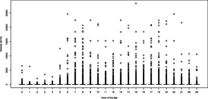
Estimated velocities of the full data
-
Vehicles: Matching the national license plates to the records of the “Vehicle Registration Service” provides additional information on these vehicles, namely vehicle kind, vehicle category and its engine’s Euronorm.
This augmented data contain 59 different vehicle kinds and 99 different vehicle categories, which is too extensive for our purpose. Instead, we group them into the following widely-used classification [29, 30]:
-
Passenger Vehicles
-
Light-Goods Vehicles (LGV): Vehicles for transporting goods with a capacity up to 3.5 tons.
-
Heavy-Goods Vehicles (HGV): Vehicles for transporting goods with a capacity above 3.5 tons.
There are some vehicles that do not match any of the above groups such as agriculture vehicles. Moreover, we do not have vehicle registration information for foreign vehicles, which account for 4% of our data. These vehicles are removed from the data in our analysis.
-
-
Zones of interest: The cameras encompass the Mechelen-Willebroek police district. It covers all the entry and exit roads of the district and more. Additionally, the city of Mechelen has a car-reduced zone. All entry and exit roads to the car-reduced zone are also covered by cameras, and it is of specific interest to the transport planners, so it is a second zone of interest. Figure 4 shows the Mechelen-Willebroek district, the car-reduced zone and the 122 ANPR camera locations.
Fig. 4 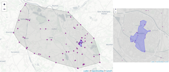
Map of Mechelen-Willebroek district, Car-reduced zone and 122 ANPR cameras


3.4 Data modeling
Our first step in modeling the data is to sort the data according to the date, vehicle identifier and time. Thereafter, we continue our modeling by data expansion as explained in the following.
-
General: For each of our observations (apart from the last observation of each vehicle), we add the next camera they go to. Thereafter, we add the time it took to get that next camera, and the distance to that camera. There can be multiple trajectories possible between two camera points. Uncertain of the road the vehicle has taken, we use the straight-line distance between the cameras. When a vehicle stops, it comes out in our analysis as vehicles with low velocities, which are identified as trip splitting points (explained in the next section). Hence, while this is an under approximation, we show in Section 5 that the speed profiles that we get are highly correlated with those from more accurate GPS data, which shows that it is a reasonable approximation. Using these measures, we can estimate the velocity of the car, which is an underestimation of the average speed it drove on the roads in between.
-
Trip identification: As we see on Fig. 3, there are many observations with low velocities. We identify three reasons for this: some vehicles leave the Mechelen-Willebroek district and come back after some time within the same day, some vehicles park for a long time, and some stop for a short time for example for a delivery or visit to a shop.
[92] and [95] define a minimum and maximum travel time between consecutive observations. If trips take longer than this maximum, they are identified as a new trip. The minimums and maximums are defined as a function of the distance between the two cameras and the distribution of travel times. We take three steps, to define the threshold to split a trip. We first determine how much time on average a vehicle takes to drive between each camera pair. The average time between each camera pair can vary according to the hour of the day. We get the average time between each camera pair per hour of working days. Thereafter, we compare the time a vehicle take to drive between the camera pair in comparison to the average time. We add to each observation what is the difference in time between the expected time and the time that it actually takes the vehicle to get there, showed in Fig. 5 (for below 120 minutes). We establish a stop according to the differences between trip duration and expected duration:
-
Stops: To determine when a vehicle stopped, we look at the difference between the actual time driven and the expected driving time between these cameras at that time of the day. Figure 5 shows the time differences over all cameras. Based on this figure, we define a stop rather conservatively as having a time difference that is more than 15 minutes, but less then 5 hours with the expected time. We have chosen these limits according to the lost time frequencies that we have been recorded, and investigating some individual movements. This can be researched further in future work.
Fig. 5 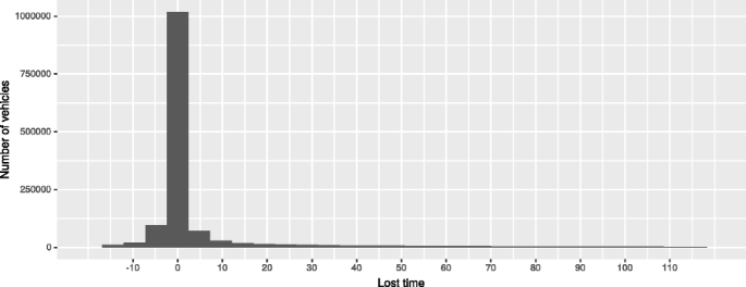
Time difference in minutes, between actual trip duration and expected duration
-
Parking or out of Region: A long stop, that is, observations where the vehicle has parked or went out of the district for a long time, are marked as such if the time that the vehicle took to get to the next camera is more than 5 hours on top of the expected time.
-

Points where a “stop” or a “long stop” have occurred are used to split the trajectories into smaller, coherent trips and our calculations are over these trips. We do not make a separation between stops that are shorter than 15 minutes.
3.5 Evaluation: visualization
In order to demonstrate the counts where e.g. number of vehicles and number of stops, and vehicles’ velocities, we have used multi-line graphs. Multi-line graphs are used to compare numbers from different vehicle categories.
For looking at the number of observations at each camera, we have used maps, where each camera is shown with a circle and the radius is related to the number of observations. Color of the circles also indicate the density of observations. A similar map has been used to show the trajectories of the vehicles, where lines thickness and colors show the trajectories taken. Finally, to display the entry-exit heat matrices are used, which use heat colors to indicate correlations between entry and exit points.
3.6 Deployment
The framework described could be deployed to provide periodic reports on the vehicle behavior, which allow to study and compare how it is evolving over time. However this paper is an exploratory study where we analyse the results of a case study of two weeks.
4 Case study on the Mechelen-Willebroek region
In this case study, we analyze data from 2 weeks, Monday 8/1/2018 to Saturday 13/1/2018 and Monday 5/2/2018 to Saturday 10/2/2018Footnote 1. The data have been analyzed for the police district of Mechelen-Willebroek in Belgium. Mechelen and Willebroek are the largest cities in the district and have 86.137 and 26.230 inhabitants respectively (2018)Footnote 2. There are 122 ANPR cameras in this police district of 92,6 square kilometres2.
All major approach roads in this district have trajectory controls with ANPR cameras [98]. Furthermore, Mechelen city has the largest car-reduced zone in Belgium, where vehicles above 10 tons are not allowed, and from 11h to 18h motorized traffic can not enter these streets without a permit. The ANPR cameras are used to enforce these regulations [98], thus essentially all approach roads have ANPR cameras.
4.1 Data quality
We provide an overview on the number of vehicles in different days of our analysis period. Figures 6 and 7 show the number of vehicles in the region and car-reduced zone respectively. We observe a similar behavior between the working days, except on "2018-01-10" where data are missing, and this day has been removed from further analysis.

Number of vehicles in the district

Number of vehicles in the car-reduced zone
Determining the number of unique vehicles in a region each day is one of the measures provided with ANPR camera data, which cannot be achieved through traditional data sources such as loops or manual counts, as they can only count on a certain point, and do not observe when the vehicle leaves the region.
We observe that the number of passenger vehicles is much larger than the number of freight vehicles. Furthermore, in the Mechelen-Willebroek district, the number of LGVs (9% of all vehicles) are around twice the number of HGVs (3.5% of all vehicles). This difference is higher in the car-reduced zone, where LGVs are 14.3% of all vehicles while HGVs are 2.7% of all vehicles. This is due to the restriction on larger vehicles in this region (no vehicles about 10 ton). We can see that freight vehicles behavior changes greatly between working days and weekends. On Saturdays, the number of HGVs decreases to a great extent. While the number of LGVs decrease as well, the difference is smaller. Finally, there are also less passengers’ vehicles on Saturdays, but the difference is not as big.
4.2 Trajectories
Insights in vehicles’ trajectories can help to locate areas that are most frequented, and hence most exposed to nuisances such as wear-and-tear of infrastructure, air pollution and noise. Depending on the area, this would indicates where policy interventions of different kinds may be desirable e.g. road maintenance, planting trees and safety measures. Especially non-primary roads, where many freight vehicles pass, deserve further attention [99].
Figures 8, 9 and 10 show the number of observations of passenger vehicles, LGVs and HGVs at different cameras respectively. The frequency in these visualizations is the average number of observations per working day.

Passengers observations

LGVs observations

HGVs observations
In addition to single-camera counts, ANPR camera data enable us to see the flow of vehicles from one camera to the other. This gives us the opportunity to look into the trajectories that are taken more often. Figures 11, 12 and 13 show the trajectories between camera pairs by passenger vehicles, LGVs and HGVs. Frequencies in these visualizations shows how many times on average working days, vehicles have driven these trajectories.

Passengers trajectories

LGVs trajectories

HGVs trajectories
We observe in both setups that the east-west road in the region is the main passage through the region. Through these figures, it is highlighted that HGVs use the secondary roads relatively less than LGVs and Passengers vehicles. LGVs are used often for smaller deliveries, e-commerce and as service vehicles such as electricians and maintenance services. Hence, this can explain their similar behavior to passenger vehicles and frequent visits to residential areas.
4.3 Entry-Exit
In Figs. 11, 12 and 13, we observed the trajectories of vehicles, monitoring frequency of vehicles traveling between each camera pair. The direction of movement is implicit. Hence, we do a complementary analysis of entry/exit flows in the region. We can observe where vehicles enter and exit the region, which provides information on the main entry and exit points and the ratio of trips from origin (row) to the destination (column). Such analysis can be done for each of the vehicle categories separately, but here we are demonstrating it for all vehicles together.
Figure 14 shows the cameras and their labels (add that A/B (former In Out) refers to different road direction), and Fig. 15 shows the entry-exit matrix with heat colors. Figure 15 shows which entry exit points are used together. In our analysis, most vehicles use the same entry point as their exit points. Furthermore, we can see that vehicles that enter from the primary roads on the west side of the district and exit from the same point as they entered, have the highest frequencies. These serve as the main gates to the district. Vehicles that enter from these points, also often exit from points that are further on the same road, which indicated the through-traffic roads. Vehicles that use three cameras on the north-west side to enter, use one point as an exit. This is the industrial zone, and vehicles entering and leaving from these points are mostly destination traffic.

Map of top cameras in Entry-Exit matrix

Entry-Exit Matrix
4.4 Hourly behavior
Transportation flows change considerably throughout the day. Looking at the number of vehicles per hour of the day allows to see this in more detail. Particularly, in light of enforced time windows such as in the car-reduced zone, analyzing hourly vehicle behavior indicates the extent to which such restrictions have effect.
Figures 16 and 17, demonstrate the number of vehicles on different hours of the days, on average working days in the Mechelen-Willebroek district and the car-reduced zone respectively.

Average number of vehicles in the region per hour

Average number of vehicles in the car-reduced zone per hour
At the district level, passenger vehicles and LGVs have two peaks, one in the morning and one in the afternoon. HGVs reach their peak between 10h and 11h, while they have a relatively consistent number during the day. HGVs start and stop driving the earliest, followed by LGVs. Passenger vehicles have the latest peak in the mornings and evenings, and their peak are the highest as well.
In the car-reduced zone, almost all freight vehicles visit before 11h, and both LGVs and HGVs barely move after that, due to the restrictions. Passenger vehicles, have the two morning and evening peaks, and their evening peak (18h-19h) is stronger.
4.5 Stops
Vehicles’ stops information provides cities insights on movements of vehicles goods, and enables adequate localization of infrastructure, e.g. parking, loading and unloading areas. As explained in Section 3.4, if a vehicle has a delay of more than 15 minutes to get to the next camera, we estimate that the vehicle has stopped during their journey. If this delay is above 5 hours, we do not consider this as a stop, but as a long stop meaning the vehicle has made a parking at their destination or has left the region during this period. The delay is the difference between the time a vehicle takes to drive between a camera pair in comparison to the average time vehicles take between the camera pairs at that hour.
Figures 18 and 19 present the number of stops estimated per hour in region and car-reduced zone. We observe that HGVs peak is earlier than LGVs, and that the peak of freight vehicles stops in the car-reduced zone is between 10 and 11h.

Average number of stops in the region per hour

Average number of stops in the car-reduced zone per hour
When we detect that there are stops between camera pairs, we associate the location of the stop to the camera, after which the stops has occurred. Figures 20, 21 and 22 show for passenger vehicles, LGVs and HGVs the cameras around which the stops have taken place. Frequencies in these visualizations show the averages on working days.

Passengers Stops

LGVs Stops

HGVs Stops
For passenger and LGVs, a camera on the south is the main point after which the vehicles are stopping. Around this camera, a retail park, distribution center of one of the chain supermarkets and the south industrial park are the main attractions. On the other hand, for the HGVs, a camera on the north-west side is the main point after which the vehicles are stopping. This region is the industrial zone in the district.
4.6 Emission standards
Based on the emission standards of the engine, each vehicle in Europe has a euro level associated with it, euro 6 being the best and euro 0 the worst. In line with cities’ efforts to control and reduce air pollution, such information indicates whether local intervention, e.g. low emission zone, is required and which vehicle categories should be targeted. Figure 23 show a comparison between the Euronorms associated with average number of LGVs vs HGVs that drive in Mechelen-Willebroek district per working day. We see that the larger vehicles have better Euronorms proportionally.

Euronorm of HGVs
4.7 Velocities
Cities are actively trying to lower vehicle speed, to decrease number of accidents. Investigating velocities, we can investigate if users respond to restrictions. Moreover, this analysis can be focused on certain sensitive roads by looking at the velocity profiles of individual cameras. Based on distances between camera pairs, and the time that vehicles take to drive between them, we estimate velocities of vehicles. Figure 24 shows the average velocity of different vehicle categories at various hours of the day. We can see that during the night there is fewer traffic (and fewer stopping), and that the morning congestion peak is worse than evening. Furthermore, there is no significant difference between vehicle categories, while HGVs have a slightly higher estimated velocity in most hours. This can be explained by the observation that HGVs drive mostly on primary road, and they go to secondary roads, where the speed limit is lower, only if they are stopping.

Velocity of Vehicles
5 Validation with gPS data
To validate accuracy and level of details in our finding from ANPR camera data, GPS data from HGVs have been used as a secondary dataset to validate the results. GPS trajectories data are a rich data source, and through this validation we compare the quality of ANPR camera data to GPS data.
As part of a dynamic road-pricing scheme in Belgium, HGVs have been equipped with On-Board Units (OBU), that submit location of the vehicle every 30 seconds to a server. Time stamp, GPS coordinates, current driving speed and direction, as measured by the GPS devices, are recorded every 30 seconds. Regarding the vehicles, the dataset contains the country code of the license plate, the European emission norm and a pseudo-identifier that changes every day at 2:00 UTC. The data have been analyzed by the methodology introduced in [55] as validation for ANPR camera data analysis. Results achieved using this methodology to analyse OBU data have been used by cities, e.g. Brussels local government.
Both ANPR cameras and OBU data, have trajectories of HGVs, which are vehicles that transport goods above 3.5 tons. On the other hand, in the ANPR camera dataset, HGVs have been categorized based on vehicle kind and category, and we may not have been able to identify all the HGVs, as sometimes the vehicle kind and category descriptions are too general. Furthermore, in the ANPR camera dataset we do not have information on vehicle kind and category of foreign vehicles, while in the OBU dataset foreign vehicles that drive in Belgium also should have an OBU. The analysis has been done for the same region as the ANPR camera data, given the convex-hull of the ANPR cameras.
In Fig. 25, we compare the number of HGVs observed with OBU and ANPR. We observe a very similar pattern but there are more unique vehicle observations with OBU. There are a number of differences between the ANPR and OBU analysis that contribute to the absolute differences: OBU data also contain foreign vehicles, ANPR data does not and also does not contain vehicles that could not be matched by the vehicle registrar (e.g. ANPR errors) or whose vehicle category is not known. The definition of heavy-good vehicle is also different for both data sources, and the OBU data are much more fine-grained and also captures vehicles that drive inbetween cameras or on highway ramps. However, with OBU there is also a danger of over-counting when vehicles start their car and drive a very short distance within a distribution center, which we have tried to detect as much as possible. The main finding is that even though there are some differences in the counts, the trends in the two datasets are the same, and can be used to monitor patterns of behavior.

Number of HGVs
Figure 26 compares the velocities calculated from ANPR cameras en OBU data. Velocities are calculated based on straight distances between observations versus time taken, and are an underestimation, as discussed before, and not the actual speed of the vehicles. OBU velocity estimates are higher, but the same trends at the peak hours, and night versus day are viewed. This confirms the validity of using straight line for velocities, as we have a small underestimation, but the rest of the information shows similar behavior and patterns. Additionally, in Fig. 27 and 28 we can observe similar trajectories when using mapmatched OBU trajectories or ANPR camera pairs. This indicates that ANPR camera data, even though much less fine-grained can reveal trajectory patterns in a region.

HGVs Velocity

OBU: HGVs Trajectories (per lane)

ANPR: HGVs trajectories (per pair counting both directions)
Finally, in Fig. 29, we see the density of stop locations from the OBU data. In Fig. 22 we also make the estimation of where HGVs stop using the ANPR camera data. While, GPS data have a higher resolution, our estimation with ANPR largely indicates the same regions as we observe with OBU. On the north-west, which is the industrial zone, we have the highest density of stops, and the other regions detected by analyzing OBU data match the observations with ANPR camera data.

OBU: HGVs Stops
We conclude from this analysis of HGV data that even though ANPR cameras have a lower coverage than GPS data, which leads to incomplete trajectories, we can still analyze and observe the main movement patterns from analyzing ANPR data. The insight such as number of vehicles, number of stops, estimated velocities, trajectories and even location of stops are all valid. The insights into number of vehicles, stops, estimated velocities, trajectories and even location of stops (albeit at a higher spatial granualarity) show the same trends, though we do observe a systematic over/under-counting for OBU/ANPR.
6 Conclusion
In the case study, we explored the potential of analyzing ANPR data for better understanding of vehicles’ movements, with a focus not just on one aspect such as travel times or stop detection, but a comprehensive approach to derive data-driven insights for city planners. We explored the vehicles movements in the region by looking at the frequency of vehicle observations by each camera, and we further analyzed that by looking into frequency of travels between each camera pair. To complement this, we investigated the entry-exit matrix, to identify the main entry and exit gates that are used together in vehicles’ trips. Furthermore, hourly behavior of vehicles in the region and specifically in the car-reduced zone was studied. In a novel approach, we also inspected frequency and location of vehicles’ stops. Finally, vehicles velocity and emission standard were also studied. In all of these analysis, we differentiate between vehicle categories, i.e light-goods vehicles, heavy-goods vehicles and passenger vehicles, and accentuate similarities and differences between these categories. These can be used by city planners to evaluate road use, road restrictions, and safety aspects, considering different categories of vehicles. Furthermore, they can monitor impact of policy measures and other changes. e.g. land use changes.
We contribute to both literature and practice by (i.) taking a holistic approach in identifying performance measures that can be derived from ANPR camera data, while most research concentrate on one aspect of transport. (ii.) Our approach for detecting stops, and estimating their location is a novel approach. (iii.) Explicit investigation of different vehicle groups (from one data source), and finding similarities and differences is often called for, and no study to date has reported on similar analysis. (iv.) We validation results of ANPR analysis using GPS data from on-board units of HGVs.
Separating passenger and freight vehicles by augmenting the data, showed that light-good vehicles behave much more like passenger vehicles, while heavy-good vehicles behave differently. More importantly, it allows to quantify what the proportion of vehicles is at the different points, which allows decision makers to consider how to best manage these flows where it matters. It also allows to monitor changes over time, e.g. for light-goods vehicles which are increasingly used for urban freight. Finally, it also allows to compare vehicle behavior per hour of the day, which showed that in the car-reduced zone almost all deliveries are before the closing of the time-window, and that this peak partly overlaps with the morning rush hour, even given that the time-window closes only at 11:00. Such insights can guide policy making regarding the choice of the size of a car-reduced zone (which impacts the peak amount of deliveries) and the timing (which impacts the amount of overlap with rush hour).
Overall we see much potential for more advanced use of ANPR cameras for monitoring and understanding vehicle behavior, especially when augmented with vehicle information. It allows to compare different types of flows in ways that were nearly impossible to quantify at that scale before.
7 Limitations and future work
Data quality The quality of the data is an important aspect when handling such big data sources. In principle, ANPR cameras register the license plate of every passing vehicle. However, there are cases where the camera system fails to read the image of the plate correctly, or where one of the letters or numbers is misread. In our case, the data were augmented with vehicle information from the national vehicle registration service, which revealed that 11% of the data entries could not be matched with vehicle information, including 4% foreign vehicles. Additionally, while the service maintains detailed information on vehicle kind and type, there were also missing values in that (presumably for older vehicles). Given the detailed categorization it was not always clear whether is a heavy-goods, light-goods or passenger one; let alone that passenger vehicles can be used to transport goods and some light-goods vehicles are actually used as family car. Other issues that impact data quality is that for privacy reasons, the license plates were hashed into a numeric ID, and as with any hash function their may be hash collisions such that two vehicles with a different plate get the same numeric ID. We indeed observed a few cases where vehicles with the same ID had different vehicle information. A final challenge we encountered is that some camera’s were much older than others, which impacts reading quality, but which also revealed that there was no mechanism in place to synchronize all the clocks. We had to remove data from 5 cameras because we could not reliably estimate the true time of the observations. To avoid this in the future, ANPR camera operators should ensure that a clock synchronization system such as NTP is in place. This stresses the importance of data quality. However, many of these issues have technical solutions (e.g. clock synchronisation, recognition accuracy, vehicle database quality) and can be expected to improve over time. Moreover, any data source has quality issues and this data should not be used to obtain to-the-number accurate records but rather good estimates of the magnitudes of volumes and of trends across time and across different locations. In that respect, ANPR cameras offer an unprecedented amount of observations, 24/7 at every installed location and for all motorized vehicles.
Camera locations ANPR data can be used to monitor not just how many vehicles pass each point, but also give an estimate of the flows. In our case study, this highlighted similar trends as did the much finer-grained GPS data. However, this also depends on the placing of the cameras. ANPR cameras are generally installed for police reasons, the most common being to monitor entry/exit points of a region (e.g the police district) or to limit access to a region (e.g. the car-reduced zone or small communes), or for section control to measure the average vehicle speed on a road and fine speed violators. It is especially these latter cameras that provide most insight into urban transport, as they are placed on key roads that have a lot of traffic passing by. The comparison with the GPS trajectories also shows where cameras may be missing to get a more complete picture. In general, placing cameras near freight zones can provide more insights into freight flows and we recommend it be considered when planning camera placement.
Data integration When more data sets are integrated, richer insights are derived. GPS data of other vehicle types, e.g. passenger, light-goods and public transport vehicles can enhance our understanding of vehicle movements greatly. Data from mobile phones can provide similar insights into vehicle movements. Contextual data can also enrich our analysis by providing a more sophisticated interpretation of any achieved results. For instance, socio-demographic data such as the number of residents in each region, shops, parking spots, etc. can provide valuable insights into the transport flows and their purpose. Additionally, our results can be combined with other data sources such as weather, accidents and, events to investigate how various environmental factors affect the transport behavior.
Driven distances In our analysis, in calculating the driven distances we have taken the length of a direct line between every two points. A higher accuracy could have been achieved, instead, by calculating the distances between the two points.
Borders In this study, our access to data has geographical limits. Hence, we do not have a full understanding of vehicle movements e.g., where their origins and destinations are if these points have been out of our data scope.
Stop detection Identifying stopping/staying points of vehicles is challenging in the analysis ANPR data. Stops are an important part of vehicle movement, as they explain many of the movements’ intentions. Furthermore, they provide valuable information for city planners on on-road stopping behavior (double parking) and the use of loading/unloading zones. We established a stop according to the differences between trip duration and expected duration. Stop detection methodology can be improved, where perhaps more of the context of the vehicle’s movements should be taken into account: what driving pattern did it have before/after, where is it, etc.
Follow-up tools The current indicators provide a snapshot view of the current situation given a set of data. This can be used to generate weekly or monthly reports. However, in such a setting the differences between the current period and the previous period also play an important role. Such a more discriminative setting, with a focus on automatically detecting trends and changes, is another avenue of future work.
Availability of data and material
Primary data are proprietary.
Notes
The dates are not the choice of the authors, and its the days that have been selected by the project commissioner.
References
Verlinde, S. (2015). Promising but challenging urban freight transport solutions: freight flow consolidation and off-hour deliveries. Brussels: Vrije Universiteit Brussel.
Kitchin, R. (2014). The real-time city? big data and smart urbanism. GeoJournal, 79(1), 1–14.
Dodge, M., & Kitchin, R. (2007). The automatic management of drivers and driving spaces. Geoforum, 38(2), 264–275.
Bommes, M., Fazekas, A., Volkenhoff, T., Oeser, M. (2016). Video based intelligent transportation systems–state of the art and future development. Transportation Research Procedia, 14, 4495–4504.
Hargrove, S.R., Lim, H., Han, L.D., Freeze, P.B. (2016). Empirical evaluation of the accuracy of technologies for measuring average speed in real time. Transportation Research Record: Journal of the Transportation Research Board, 73–82.
Shin, D., Aliaga, D., Tunçer, B., Arisona, S.M., Kim, S., Zünd, D., Schmitt, G. (2015). Urban sensing: Using smartphones for transportation mode classification. Computers, Environment and Urban Systems, 53, 76–86.
Allen, J., Ambrosini, C., Browne, M., Patier, D., Routhier, J.-L., Woodburn, A. (2014). Data collection for understanding urban goods movement. In Sustainable Urban Logistics: Concepts, Methods and Information Systems. https://doi.org/10.1007/978-3-642-31788-0_5. Springer, (pp. 71–89).
Zheng, Y., Zhang, L., Xie, X., Ma, W.-Y. (2009). Mining interesting locations and travel sequences from gps trajectories. In Proceedings of the 18th international conference on World wide web - WWW ’09. https://doi.org/10.1145/1526709.1526816. ACM.
Cheung, S.Y., Coleri, S., Dundar, B., Ganesh, S., Tan, C.-W., Varaiya, P. (2005). Traffic measurement and vehicle classification with single magnetic sensor. Transportation Research Record, 1917(1), 173–181.
Kan, Z., Tang, L., Kwan, M.-P., Ren, C., Liu, D., Li, Q. (2018). Traffic congestion analysis at the turn level using taxis’ gps trajectory data. Computers, Environment and Urban Systems. https://doi.org/10.1016/j.compenvurbsys.2018.11.007.
Zhang, D.-Z., Peng, Z.-R., Sun, D.J. (2014). A comprehensive taxi assessment index using floating car data. Washington, DC: Transportation Research Board.
Moreira-Matias, L., Gama, J., Ferreira, M., Mendes-Moreira, J., Damas, L. (2013). Predicting taxi–passenger demand using streaming data. IEEE Transactions on Intelligent Transportation Systems, 14(3), 1393–1402.
Yao, E.J., Pan, L., Yang, Y., Zhang, Y.S. (2013). Taxi driver’s route choice behavior analysis based on floating car data. In Applied Mechanics and Materials, (Vol. 361. Trans Tech Publ, Switzerland, pp. 2036–2039).
Nguyen, K., Yang, J., Lin, Y., Lin, J., Chiang, Y.-Y., Shahabi, C. (2018). Los angeles metro bus data analysis using gps trajectory and schedule data (demo paper). In Proceedings of the 26th ACM SIGSPATIAL International Conference on Advances in Geographic Information Systems. https://doi.org/10.1145/3274895.3274911. ACM.
Bie, Y., Gong, X., Liu, Z. (2015). Time of day intervals partition for bus schedule using gps data. Transportation Research Part C: Emerging Technologies, 60, 443–456.
Eran, T., Boaz, L., Eyal, B.Z., Irad, B-G. (2018). Analyzing large-scale human mobility data: a survey of machine learning methods and applications. Knowledge and Information Systems. https://doi.org/10.1007/s10115-018-1186-x.
Pappalardo, L., Simini, F., Rinzivillo, S., Pedreschi, D., Giannotti, F., Barabási, A.-L. (2015). Returners and explorers dichotomy in human mobility. Nature communications, 6(1). https://doi.org/10.1038/ncomms9166.
Ampt, E., Davis, M., Stark, E. (2018). Monitoring car use over extended period with gps devices – retaining response rates and understanding reactions. Transportation Research Procedia, 32, 242–252. https://doi.org/10.1016/j.trpro.2018.10.046. Transport Survey Methods in the era of big data:facing the challenges.
Ezzat, M., Sakr, M., Elgohary, R., Khalifa, M.E. (2018). Building road segments and detecting turns from gps tracks. Journal of Computational Science, 29, 81–93. https://doi.org/10.1016/j.jocs.2018.09.011.
Dulebenets, M.A., Pujats, K., Deligiannis, N. (2017). Development of tools for processing truck gps data and analysis of freight 1 transportation facilities 2. Transportation, 2, 3.
Zanjani, A.B., Pinjari, A.R., Kamali, M., Thakur, A., Short, J., Mysore, V., Tabatabaee, S.F. (2015). Estimation of statewide origin–destination truck flows from large streams of gps data. Transportation Research Record: Journal of the Transportation Research Board, 2494, 87–96.
Sturm, K., Pourabdollahi, Z., Mohammadian, A., Kawamura, K. (2014). Gps and driver log-based survey of grocery trucks in chicago, illinois. Transportation Research Record: Journal of the Transportation Research Board, 31–38.
Yang, X., Sun, Z., Ban, X.J., Wojtowicz, J., Holguín-Veras, J. (2014). Urban freight performance evaluation using gps data. In Transportation Research Board (TRB) 93rd Annual Meeting, Vol. 600, Washington, D.C., (p. 45).
Dablanc, L. (2007). Goods transport in large european cities: Difficult to organize, difficult to modernize. Transportation Research Part A: Policy and Practice, 41(3), 280–285.
Campagna, A., Stathacopoulos, A., Persia, L., Xenou, E. (2017). Data collection framework for understanding uft within city logistics solutions. Transportation Research Procedia, 24, 354–361.
Rai, H.B., van Lier, T., Meers, D., Macharis, C. (2017). Improving urban freight transport sustainability: Policy assessment framework and case study. Research in Transportation Economics, 64, 26–35.
Kaszubowski, D. (2017). Urban freight transport demand modelling and data availability constraints. In Scientific And Technical Conference Transport Systems Theory And Practice. https://doi.org/10.1007/978-3-319-62316-0_14. Springer, (pp. 172–182).
Cherrett, T., Allen, J., McLeod, F., Maynard, S., Hickford, A., Browne, M. (2012). Understanding urban freight activity–key issues for freight planning. Journal of Transport Geography, 24, 22–32.
TransportPolicy.net (2018). EU: VEHICLE DEFINITIONS. https://www.transportpolicy.net/standard/eu-vehicle-definitions/. Accessed 19 Nov 2018.
Comission, E. (2018). Vehicle categories. http://ec.europa.eu/growth/sectors/automotive/vehicle-categories/. Accessed 29 Nov 2018.
Chapman, P., Clinton, J., Kerber, R., Khabaza, T., Reinartz, T., Shearer, C., Wirth, R. (2000). Crisp-dm 1.0 step-by-step data mining guide. Technical report. The CRISP-DM consortium. http://www.crisp-dm.org/CRISPWP-0800.pdf. Accessed 19 Nov 2018.
Coifman, B. (2007). Vehicle classification from single loop detectors. Technical report.
Coifman, B. (2002). Estimating travel times and vehicle trajectories on freeways using dual loop detectors. Transportation Research Part A: Policy and Practice, 36(4), 351–364.
Chen, C., Petty, K., Skabardonis, A., Varaiya, P., Jia, Z. (2001). Freeway performance measurement system: mining loop detector data. Transportation Research Record: Journal of the Transportation Research Board, 96–102.
Bremmer, D., Cotton, K., Cotey, D., Prestrud, C., Westby, G. (2004). Measuring congestion: Learning from operational data. Transportation Research Record: Journal of the Transportation Research Board, 188–196.
Palen, J., Coifman, B., Sun, C., Ritchie, S.G., Varaiya, P. (2000). California partners for advanced transit and highways (path) enhanced loop-based traffic surveillance program. ITS quarterly, 8(4).
D’Angelo, M., Al-Deek, H., Wang, M. (1999). Travel-time prediction for freeway corridors. Transportation Research Record: Journal of the Transportation Research Board, 184–191.
Zhang, X., Wang, Y., Nihan, N.L., Dong, H. (2005). Monitoring a freeway network in real time using single-loop detectors. International journal of vehicle information and communication systems, 1(1-2), 119–130.
Mazaré, P.-E., Tossavainen, O.-P., Bayen, A., Work, D. (2012). Trade-offs between inductive loops and gps probe vehicles for travel time estimation: A mobile century case study. In Transportation Research Board 91st Annual Meeting (TRB’12), vol. 349.
Kwon, J., Petty, K., Varaiya, P. (2007). Probe vehicle runs or loop detectors?: Effect of detector spacing and sample size on accuracy of freeway congestion monitoring. Transportation Research Record: Journal of the Transportation Research Board, 57–63.
Herrera, J.C., & Bayen, A.M. (2010). Incorporation of lagrangian measurements in freeway traffic state estimation. Transportation Research Part B: Methodological, 44(4), 460–481.
Friesen, M.R., & McLeod, R.D. (2015). Bluetooth in intelligent transportation systems: a survey. International Journal of Intelligent Transportation Systems Research, 13(3), 143–153.
Li, P., & Souleyrette, R.R. (2016). A generic approach to estimate freeway traffic time using vehicle id-matching technologies. Computer-Aided Civil and Infrastructure Engineering, 31(5), 351–365.
Zinner, S. (2012). A methodology for using bluetooth to measure real-time work zone travel time. PhD thesis. Atlanta: Georgia Institute of Technology.
Yildirimoglu, M., & Kim, J. (2018). Identification of communities in urban mobility networks using multi-layer graphs of network traffic. Transportation Research Part C: Emerging Technologies, 89, 254–267.
Duivenbooden, T.F. (2012). Route choice modelling based on empirical evidence: case study alkmaar. Master’s thesis,.
Leduc, G. (2008). Road traffic data: Collection methods and applications. Working Papers on Energy, Transport and Climate Change, 1(55), 1–55. European Commission Joint Research Centre Institute for Prospective.
Li, M., Chen, X., Ni, W. (2016). An extended generalized filter algorithm for urban expressway traffic time estimation based on heterogeneous data. Journal of Intelligent Transportation Systems, 20(5), 474–484.
Yang, C., Ma, X., Ban, Y. (2016). Demonstration of intelligent transport applications using freight transport gps data. In Transportation Research Board 95th Annual Meeting.
Short, J. (2014). Truck gps data for tracking freight flows. In Developing Freight Fluidity Performance Measures. Summary of a Workshop. Transportation Research Circular Number E-C187, (pp. 35–38).
Srour, F., & Newton, D. (2006). Freight-specific data derived from intelligent transportation systems: Potential uses in planning freight improvement projects. Transportation Research Record: Journal of the Transportation Research Board, 66–74.
Gabrielli, L., Furletti, B., Trasarti, R., Giannotti, F., Pedreschi, D. (2015). City users’ classification with mobile phone data. In 2015 IEEE International Conference on Big Data (Big Data). https://doi.org/10.1109/bigdata.2015.7363852.
Pappalardo, L., Pedreschi, D., Smoreda, Z., Giannotti, F. (2015). Using big data to study the link between human mobility and socio-economic development. In 2015 IEEE International Conference on Big Data (Big Data). https://doi.org/10.1109/bigdata.2015.7363835. IEEE, (pp. 871–878).
Gonçalves, J., Gonçalves, J.S., Rossetti, R.J., Olaverri-Monreal, C. (2014). Smartphone sensor platform to study traffic conditions and assess driving performance. In 17th International IEEE Conference on Intelligent Transportation Systems (ITSC). https://doi.org/10.1109/itsc.2014.6958106. IEEE, (pp. 2596–2601).
Hadavi, S., Verlinde, S., Verbeke, W., Macharis, C., Guns, T. (2018). Monitoring urban-freight transport based on gps trajectories of heavy-goods vehicles. IEEE Transactions on Intelligent Transportation Systems, 20(10), 3747–3758. IEEE.
Gingerich, K., Maoh, H., Anderson, W. (2016). Classifying the purpose of stopped truck events: An application of entropy to gps data. Transportation Research Part C: Emerging Technologies, 64, 17–27.
Liao, C.-F. (2009). Using archived truck gps data for freight performance analysis on i-94/i-90 from the twin cities to chicago. University of Minnesota Center for Transportation Studies.
Bar-Gera, H. (2007). Evaluation of a cellular phone-based system for measurements of traffic speeds and travel times: A case study from Israel. Transportation Research Part C: Emerging Technologies, 15(6), 380–391.
ZHANG, C., Xiaoguang, Y., Xinping, Y. (2007). Journal of Transportation Systems Engineering and Information Technology, 7(3), 100–104.
Astarita, V., Bertini, R.L., d’Elia, S., Guido, G. (2006). Motorway traffic parameter estimation from mobile phone counts. European Journal of Operational Research, 175(3), 1435–1446.
Pan, C., Lu, J., Di, S., Ran, B. (2006). Cellular-based data-extracting method for trip distribution. Transportation research record, 1945(1), 33–39.
Ma, J., Li, H., Yuan, F., Bauer, T. (2013). Deriving operational origin-destination matrices from large scale mobile phone data. International Journal of Transportation Science and Technology, 2(3), 183–204.
Zhang, Y., Qin, X., Dong, S., Ran, B. (2010). Daily od matrix estimation using cellular probe data. In 89th Annual Meeting Transportation Research Board, vol. 9.
Patel, C., Shah, D., Patel, A. (2013). Automatic number plate recognition system (anpr): A survey. International Journal of Computer Applications, 69(9).
Rhead, M., Gurney, R., Ramalingam, S., Cohen, N. (2012). Accuracy of automatic number plate recognition (anpr) and real world uk number plate problems. In 2012 IEEE International Carnahan Conference on Security Technology (ICCST). https://doi.org/10.1109/ccst.2012.6393574. IEEE.
Debnath, A.K., Chin, H.C., Haque, M.M., Yuen, B. (2014). A methodological framework for benchmarking smart transport cities. Cities, 37, 47–56.
DutchNews (2018). Criminals caught on camera: police expand camera surveillance on roads. https://www.dutchnews.nl/news/2017/11/criminals-caught-on-camera-police-expand-camera-surveillance-on-roads/. Accessed 19 Nov 2018.
EDRI (2018). Denmark: Targeted ANPR data retention turned into mass surveillance. https://edri.org/denmark-targeted-anpr-data-retention-turned-into-mass-surveillance/. Accessed 19 Nov 2018.
Dynamics, S. (2018). Sensor Dynamics. https://www.sensordynamics.com.au/. Accessed 19 Nov 2018.
Joris, L. (2018). Up to 3.000 cameras on Belgian road network. https://newmobility.news/2018/08/21/up-to-3-000-cameras-on-belgian-road-network/. Accessed 19 Nov 2018.
Pirc, J., Turk, G., žura, M. (2016). Highway travel time estimation using multiple data sources. IET Intelligent Transport Systems, 10(10), 649–657.
Yasin, A.M., Karim, M.R., Abdullah, A.S. (2010). Travel time measurement in real-time using automatic number plate recognition for malaysian environment. Journal of the Eastern Asia Society for Transportation Studies, 8, 1738–1751.
Kanayama, K., Fujikawa, Y., Fujimoto, K., Horino, M. (1991). Development of vehicle-license number recognition system using real-time image processing and its application to travel-time measurement. In [1991 Proceedings] 41st IEEE Vehicular Technology Conference. https://doi.org/10.1109/vetec.1991.140605. IEEE.
Chow, A.H., Santacreu, A., Tsapakis, I., Tanasaranond, G., Cheng, T. (2014). Empirical assessment of urban traffic congestion. Journal of advanced transportation, 48(8), 1000–1016.
Bradley, J., Kaenzig, R., Harris, J., Sanclemente, J., Cottam, M., Stringer, R., Corr, G., Hicks, D. (2017). Understanding and managing congestion for transport for London. Technical report. http://content.tfl.gov.uk/understanding-and-managing-congestion-in-london.pdf.
Robinson, S., & Polak, J. (2006). Overtaking rule method for the cleaning of matched license-plate data. Journal of transportation engineering, 132(8), 609–617.
Burton, P., Crosthwaite, S., Simpson, A., Billington, P. (2008). The design and implementation of a national real-time travel time on vms service. In 15th World Congress on Intelligent Transport Systems and ITS America’s 2008 Annual MeetingITS AmericaERTICOITS JapanTransCore, New York.
Asamer, J., Graser, A., Prandtstetter, M., Ruthmair, M. (2016). Optimizing checkpoints for arrival time prediction. In Proceedings of the 7th International Conference on Computational Logistics, ICCL’16, (p. 86).
Bertini, R.L., Lasky, M., Monsere, C.M. (2005). Validating predicted rural corridor travel times from an automated license plate recognition system: Oregon’s frontier project. In Proceedings. 2005 IEEE Intelligent Transportation Systems, 2005. https://doi.org/10.1109/itsc.2005.1520134. IEEE, (pp. 296–301).
Hargrove, S.R.A. (2015). Self-learning license plate matching algorithm: Some enhancements and its role in travel time ground truth measurements. Knoxville: University of Tennessee.
Friedrich, M., Jehlicka, P., Schlaich, J. (2008). Automatic number plate recognition for the observance of travel behavior. Proc., the 8th International Conference on Survey Methods in Transport.
Ryguła, A., Maczyński, A., Piwowarczyk, P. (2014). Evaluating the efficiency of road traffic management system in chorzow. In Telematics - Support for Transport. https://doi.org/10.1007/978-3-662-45317-9_45. Springer, (pp. 424–433).
Mo, B., Li, R., Zhan, X. (2017). Speed profile estimation using license plate recognition data. Transportation research part C: emerging technologies, 82, 358–378.
Zhan, X., Li, R., Ukkusuri, S.V. (2015). Lane-based real-time queue length estimation using license plate recognition data. Transportation Research Part C: Emerging Technologies, 57, 85–102.
Robinson, A., & Van Niekerk, A. (2014). Uses of anpr data in traffic management and transport modelling. In Proceedings of the 33rd Southern African Transport Conference (SATC 2014), (Vol. 7. Citeseer, p. 10).
Castillo, E., Menéndez, J.M., Jiménez, P. (2008). Trip matrix and path flow reconstruction and estimation based on plate scanning and link observations. Transportation Research Part B: Methodological, 42(5), 455–481.
Castillo, E., Gallego, I., Menéndez, J.M., Rivas, A. (2010). Optimal use of plate-scanning resources for route flow estimation in traffic networks. IEEE Transactions on Intelligent Transportation Systems, 11(2), 380–391.
Yu, H., Yang, S., Wu, Z., Ma, X. (2018). Vehicle trajectory reconstruction from automatic license plate reader data. International Journal of Distributed Sensor Networks, 14(2), 1550147718755637.
Khoeini, S., Rodgers, M., Elango, V., Guensler, R. (2012). Sensitivity of commuters’ demographic characteristics to license plate data collection specifications: Case study of i-85 high-occupancy vehicle to high-occupancy toll lanes conversion in atlanta, georgia. Transportation Research Record: Journal of the Transportation Research Board, 2308, 37–46.
Li, R., Liu, Z., Zhang, R. (2018). Studying the benefits of carpooling in an urban area using automatic vehicle identification data. Transportation Research Part C: Emerging Technologies, 93, 367–380.
Mcleod, F., Cherrett, T., Box, S., Waterson, B., Pritchard, J. (2017). Using automatic number plate recognition data to investigate the regularity of vehicle arrivals. European Journal of Transportation and Infrastructure Research, 17(1), 86–102.
Silva, P.M.P., Forshaw, M., McGough, A.S. (2018). Clustering vehicles based on trips identified from automatic number plate recognition camera scans. In 1st International Workshop on Big Traffic Data Analytics (BigTraffic 2018.
Chen, H., Yang, C., Xu, X. (2017). Clustering vehicle temporal and spatial travel behavior using license plate recognition data. Journal of Advanced Transportation, 2017, 1–14. https://doi.org/10.1155/2017/1738085.
Sun, Y., Zhu, H., Zhou, X., Sun, L. (2014). Vapa: Vehicle activity patterns analysis based on automatic number plate recognition system data. Procedia Computer Science, 31, 48–57.
Homayounfar, A., Ho, A., Zhu, N., Head, G., Palmer, P. (2011). Multi-vehicle convoy analysis based on anpr data. In 4th International Conference on Imaging for Crime Detection and Prevention 2011 (ICDP 2011). https://doi.org/10.1049/ic.2011.0135. IET.
Kuroiwa, H., & Kamijo, S. (2007). Directional travel time measurement by surveillance camera network. In 2007 IEEE International Conference on Systems, Man and Cybernetics. https://doi.org/10.1109/icsmc.2007.4413637. IEEE, (pp. 1699–1704).
Zmud, J., Wagner, J., Moran, M., George, J.P. (2016). License plate reader technology: Transportation uses and privacy risks.
Van Haezendonck, S. (2016). Mechelen puts city full of section checks and lorry locks. Nieuwsblad.
Briassoulis, H. (2001). Sustainable development and its indicators: through a (planner’s) glass darkly. Journal of Environmental Planning and Management, 44(3), 409–427.
Acknowledgements
This work was supported by the European Regional Development Fund (ERDF) and the Brussels-Capital Region-Innoviris within the framework of the Operational Programme 2014-2020 through the ERDF-2020 project ICITY-RDI.BRU.
Funding
Not applicable.
Author information
Authors and Affiliations
Contributions
SH and TG coordinated the data collection, performed the data analytics and manuscript writing. HBR and SV contributed to meta-analysis and content planning. All authors provided feedback in every step, reviewed the results and approved the final version of the manuscript.
Corresponding author
Ethics declarations
Competing interests
On behalf of all authors, the corresponding author states that there is no conflict of interest.
Additional information
Publisher’s Note
Springer Nature remains neutral with regard to jurisdictional claims in published maps and institutional affiliations.
Rights and permissions
Open Access This article is licensed under a Creative Commons Attribution 4.0 International License, which permits use, sharing, adaptation, distribution and reproduction in any medium or format, as long as you give appropriate credit to the original author(s) and the source, provide a link to the Creative Commons licence, and indicate if changes were made. The images or other third party material in this article are included in the article’s Creative Commons licence, unless indicated otherwise in a credit line to the material. If material is not included in the article’s Creative Commons licence and your intended use is not permitted by statutory regulation or exceeds the permitted use, you will need to obtain permission directly from the copyright holder. To view a copy of this licence, visit http://creativecommons.org/licenses/by/4.0/.
About this article

Cite this article
Hadavi, S., Rai, H.B., Verlinde, S. et al. Analyzing passenger and freight vehicle movements from automatic-Number plate recognition camera data. Eur. Transp. Res. Rev. 12, 37 (2020). https://doi.org/10.1186/s12544-020-00405-x
Received:
Accepted:
Published:
DOI: https://doi.org/10.1186/s12544-020-00405-x