Locomotive assignment problem with train precedence using genetic algorithm

Abstract

This paper aims to study the locomotive assignment problem which is very important for railway companies, in view of high cost of operating locomotives. This problem is to determine the minimum cost assignment of homogeneous locomotives located in some central depots to a set of pre-scheduled trains in order to provide sufficient power to pull the trains from their origins to their destinations. These trains have different degrees of priority for servicing, and the high class of trains should be serviced earlier than others. This problem is modeled using vehicle routing and scheduling problem where trains representing the customers are supposed to be serviced in pre-specified hard/soft fuzzy time windows.

A two-phase approach is used which, in the first phase, the multi-depot locomotive assignment is converted to a set of single depot problems, and after that, each single depot problem is solved heuristically by a hybrid genetic algorithm. In the genetic algorithm, various heuristics and efficient operators are used in the evolutionary search. The suggested algorithm is applied to solve the medium sized numerical example to check capabilities of the model and algorithm. Moreover, some of the results are compared with those solutions produced by branch-and-bound technique to determine validity and quality of the model. Results show that suggested approach is rather effective in respect of quality and time.

Background

The rail transportation industry has many problems that can be modeled by mathematical programming and solved using soft computing techniques. But the research in railroad scheduling has experienced a slow growth (Ahuja et al.[2005]). A growing interest for using optimization techniques in railroad problems has appeared in the operation research literature (see, e.g., Brannlund et al. ([1998]) and Cordeau et al. ([1998])). One of the most important problems in rail transportation industry in view of operating costs is locomotive assignment or locomotive routing and scheduling problem. Because the considerable cost usually is paid by rail companies for operating the locomotives according to the properly assignment plan that has a direct impact on operating cost, punctuality and performance, which in turn affect customers' satisfaction, finding a way to design a proper locomotive assignment and scheduling policy can be an important decision in railroad companies. The planning stage in railroad scheduling is divided to strategic, tactical and operational planning. These stages are in accordance with the length of the respective planning horizon and the temporal impact and relevance of the decision. According to these levels of planning, locomotive scheduling is the final stage of the railroad scheduling and depends on incoming requests, but with this assumption, engines and crews are rostered and appropriate cars are available. It must be mentioned that this paper is a complementary version of our recent researches (Ghoseiri and Ghannadpour[2009a];[Ghoseiri and Ghannadpour 2010]) about the locomotive assignment problem. Ghoseiri and Ghannadpour ([2009a]) suggested the solving of the general locomotive planning (or scheduling) that is one of the most attractive topics in operation research by vehicle routing problem.[Ghoseiri and Ghannadpour (2010]) extended the previous research and tried to study the multi-depot homogenous locomotive assignment with more real-life assumptions. This model was formulated by vehicle routing problem with time windows (VRPTW) and solved heuristically by an efficient hybrid genetic algorithm. This paper, in continuation of previous researches, tries to consider the different degrees of priority of trains for servicing using the concept of fuzzy time windows.

As mentioned earlier, few references can be found in the literature regarding operation research for assignment of locomotives to trains. A version of the problem, where a single locomotive must be assigned to each train, no deadhead is allowed, and no maintenance requirements are taken into account was addressed by Forbes et al. ([1991]). In an earlier paper, Florian et al. ([1976]) introduced an integer programming model based on a multi-commodity network for the case where several locomotives can be assigned to each train. Ziarati et al. ([1997]) extended Florian et al. ([1976]) formulation to include almost all the operational constraints encountered at CN North America. Ahuja et al. ([2005]) presented the real-life locomotive scheduling faced by CSX transportation (Jacksonville, Florida), a major US railroad company. They considered the planning version of the locomotive scheduling model, where there were multiple types of locomotives and needed to decide the set of locomotives to be assigned to each train. A Benders decomposition approach to the locomotive assignment problem can be found in Cordeau et al. ([2000]). In a subsequent paper, Cordeau et al. ([2001a]) extended the previous work with various real-life constraints, such as maintenance. Rouillon et al. ([2006]) presented an efficient backtracking mechanism that can be added to this heuristic branch-and-price approach. Moreover, Vaidyanathan et al. ([2008b]) developed new formulations for the locomotive planning problem (LPP). In this paper, new constraints were added to the planning problem desired by locomotive directors, and additional formulations necessary to transition solutions of models to practice were developed. Also, two formulations namely consist formulation and hybrid formulation were suggested for this generalized LPP.

In this area, Vaidyanathan et al. ([2008a]) developed robust optimization methods to solve the LPP. In this paper, two major sets of constraints were considered and should have satisfied by each locomotive route: (1) locomotive fueling constraints, which requires that every unit visit of a fueling station be conducted at least once for every F miles of travel, and (2) locomotive servicing constraints, which require that every unit visit of a service station be conducted at least once for every S miles of travel. This problem was formulated as an integer programming problem on a suitably constructed space-time network, and it was shown that this problem is NP-complete. Other important locomotive assignment papers can be found in Cordeau et al. ([2001b]), Fioole et al. ([2006]), Lingaya et al. ([2002]), etc.

As mentioned earlier, the model that is considered in this paper is presented using the vehicle routing and scheduling problem in which the trains are supposed to be serviced in pre-specified hard/soft fuzzy time windows. This problem is an important variant of vehicle routing problem (VRP) with adding time window constraints to the model in which a set of vehicles with limited capacity is to be routed from a central depot to a set of geographically dispersed customers with known demands and predefined time windows in order that fleet size of vehicles and total traveling distance are minimized, and capacity and time windows constraints are not violated. Usually, in real world VRPs, many side constraints appear. Because of many applications of different kinds of VRP problems, many researchers have focused to develop solution approaches for these problems. We can find useful techniques for the general VRP in Bräysy and[Gendreau (2001]),[Laporte and Semet (1999]), and[Pisinger and Ropke (2007]). In this area,[Czech and Czarnas (2002]) solved VRPTW with simulated annealing, and Gambardella et al. ([1999]) applied multiple ant colony system for VRPTW. Alvarenga et al. ([2007]),[Berger and Barkaoui (2003]), Ghoseiri and Ghannadpour ([2009b]), and Tan et al. ([2006]) used genetic algorithm for VRPTW. Other very good techniques and applications of VRPTW can be found in[Cerda and Dondo (2007]), Crevier et al. ([2007]), Irnich et al. ([2006]), Kim et al. ([2006]), Li et al. ([2005]), and Tan et al. ([2007]). As mentioned earlier, this paper uses the concept of fuzzy approach to consider the different degrees of priority of trains for servicing. This concept is known as fuzzy time windows in the literature of VRP models in which the customers hop to be served at desired time if possible. The most important studies in this area can be found in Sheng et al. ([2006]) and Cheng et al. ([1996]). According to literature, the suggested model based on VRPTW with fuzzy concept is NP-hard, and due to the intrinsic difficulty of the problem, heuristic methods are most promising for solving it. In this paper, among the number of solving methods which were explored, genetic algorithm is examined in greater depth and combined with other heuristics to solve the suggested model.

The remaining parts of paper are organized as follows: ‘Locomotive assignment with train precedence’ section defines the locomotive assignment problem with fuzzy time windows. ‘Solution procedure’ section introduces the hybrid genetic search algorithm to solve the problem. ‘Numerical example and results analysis’ section discusses the model validation and computational complexity of the proposed method, and ‘Conclusion’ section provides the concluding remarks.

Results and discussion

This section describes computational experiments carried out to investigate the performance of the proposed GA. The algorithm was coded in MATLAB 7 and run on a PC with 1.6-GHz CPU and 512-MB memory. In this section, a complete randomly generated medium size problem is considered as a numerical example. Before solving and analyzing this problem, the validity and quality of suggested method should be checked. So, a few small- and medium-sized problems are created and solved by branch-and-bound (B&B) technique. The solutions yielded by the exact optimization technique are compared with those of the hybrid algorithm in general approach. Table 1 summarizes the results.

Table 1 Comparing the results with exact solutions

The times that are reported in column CPU time (Loco-GA) are the times to find the best solutions of each test problem during the 600 generations. In comparison with the exact solution of branch-and-bound technique, the hybrid GA algorithm has a zero percentage of error and drastically reduces the CPU time for the generated test problems. Also, in order to determine computational complexity of the algorithm, 15 instance problems are solved ranging from 10 to 100 trains which the produced results are illustrated in Figure 1. With reference to results, the computational complexity of the algorithm falls between n² and nlog (n), i.e., the hybrid genetic algorithm solve a NP-hard problem in a polynomial time computation that is an advantage for the algorithm.

Figure 1

Typical routes with and without waiting time.

Now, a randomly generated medium size problem should be considered. It includes 80 nodes and 40 trains per day in a weekly planning horizon. Ten trains are considered high class, and the fuzzy time windows with different widths are considered for them. These trains have to be serviced without any delay, and their satisfaction for receiving services should be maximized. A maximum permissible operating time of 18 h is defined for all the trains running in the planning horizon, and maintenance time for each locomotive is assumed to be 6 h. The locomotive speed is variable at different points of route in accordance with a normal probability distribution from 45 to 65 km/h. At first, this problem is solved in which all trains are considered normal, and they have classical time windows. Then, 10 trains are selected randomly, and they are supposed to be high class with different fuzzy time windows. So, at first stage, nine locomotives are needed to service all trains with classical time windows. The total traveling time of this solution is 64.93 h; total traveling distance is 3,386.4 km; and the total waiting time is 8.4 h. Also, the order of servicing is shown in Figure 2.

Figure 2

Best solution of problem in 600 generations (classical time windows).

With reference to Figure 2, each locomotive according to its constructed route services to the trains en route. For instance, the sixth locomotive starts its journey at depot and hauls trains 21, 39, 28 and 5 to their destinations and then returns to the central depot for its routine daily maintenance. In fact, the sixth locomotive goes to the origin node of the 21st train zone and hauls the train to its destination, and then goes to the origin node of the 39th train zone and keeps on going, i.e., the sixth route is as follows:

$$\left\{O_{21},D_{21},O_{39},D_{39},O_{28},D_{28},O_5,D_5\right\}\text{.}$$

At the second stage, ten trains are selected randomly, and they were considered as high priority trains. These trains are highlighted in Figure 2. According to these changes, the locomotive assignment model was solved again, and the produced result is shown in Figure 3.

Figure 3

Best solution of problem in 600 generations (ten high class trains).

According to this figure, nine locomotives are needed for serving all trains. The total traveling time of this solution is 65.93 h, total traveling distance is 3586.7 km and the total waiting time is 6.15 h. Also, the order of servicing is changed to maximize the satisfaction rate of trains with high degree of priority. Considering the ten high class trains, the summation of satisfaction rate for this solution is 30.7, while this rate for the solution of Figure 2 is 27.1. So, the algorithm tries to change the servicing arrangement of trains to earn more value of satisfaction. For example, for train 7 which is considered as high priority train, the satisfaction rate was 0.27 in previous solution and increased to 0.61 in the new solution by changing to arrival time of locomotive and servicing arrangement. Hence, the suggested algorithm for serving the trains tries to maximize the satisfaction rate of high priority trains considering the other objectives, namely, traveling time, distance and waiting time.

Moreover, an operator deletion-retrieval strategy is executed to probe the efficiency of the inner working of the suggested method. According to this strategy, genetic operators are eliminated one at a time and each time. Algorithm is put into run, and convergence behavior is studied and compared with the operator retrieved. Figure 4 summarizes the analysis of the operator's effect on convergence behavior of the hybrid genetic algorithm for a test problem.

Figure 4

Inner working of method under the operation of different operators.

According to Figure 4, the hill climbing operator has the main role to improve the chromosomes obtained through crossover and mutation, and it works highly efficient. Figure 4 shows that all the inner components of the hybrid genetic algorithm work properly and indicate good behavior of convergence towards the best solutions.

As mentioned earlier, this paper used an adaptive mutation probability scheme, which changed the mutation probability as the standard deviation of the population fitness changes. This scheme was proposed to maintain and control the diversification of population in each generation. Figure 5 illustrates the behavior of this scheme in the first 200 generations of a test problem. According to this figure, the mutation probability (upside schema) should be increased when the diversification of population is decreased. Also, this probability should be decreased to maintain the population diversification when the standard deviation of the population fitness changes is increased.

Figure 5

Inner working of method under the operation of different operators.

As mentioned earlier, this paper tried to check the effectiveness of other crossover operators, namely, route exchange crossover (REX) versus the heuristic and merge crossover (HMX). To check the efficiency of these operators, a comparison is undertaken between these operators and partially mapped crossover (PMX) which is the common operator for sequential problem like TSP and VRP. Figure 6 illustrates this comparison.

Figure 6

Comparison between REX, HMX, and PMX.

Unlike PMX and HMX, which were used in our recent research ([Ghoseiri and Ghannadpour 2010]), the REX that is suggested in this paper produces better solution and works properly than them. Eventually, produced results show that suggested approach is quiet effective in respect of quality and time.

Conclusion

This paper presented the locomotive assignment problem which is very important for railway companies, in view of high cost of operating locomotives. This problem was to determine the minimum cost assignment of homogeneous locomotives located in some central depots to a set of pre-scheduled trains in order to provide sufficient power to pull the trains from their origins to their destinations. These trains had different degrees of priority for servicing, and the high class of trains should have serviced earlier than others. This problem was modeled using vehicle routing and scheduling problem where trains performed as customers, and they should have serviced in pre-specified hard/soft fuzzy time windows.

A two-phase approach was used in which, in the first phase, the multi-depot locomotive assignment was converted to a set of single depot problems, and after that, each single depot problem was solved heuristically by a hybrid genetic algorithm. In the genetic algorithm, various heuristics and efficient operators were used in the evolutionary search.

In suggested algorithm, the push-forward insertion heuristic (PFIH) was used to determine the initial solution, and λ-interchange mechanism was used for neighborhood search and improving method. Moreover, new crossover operator was suggested and it was shown that it worked more properly than the old operators.

The suggested algorithm was applied to solve the medium-sized numerical example to check capabilities of the model and algorithm. Moreover, some of the results were compared with those solutions produced by branch-and-bound technique to determine validity and quality of the model. Results indicated that this algorithm was efficient and solved the problem in a polynomial time.

Methods

Locomotive assignment with train precedence

The problem includes a set of homogeneous locomotives, a set of depots where locomotives are initially located, and a set of pre-scheduled trains with different degrees of priority (e.g., normal passenger trains, high speed trains, freight trains, etc.). As mentioned earlier, this problem is modeled by VRPTW. In this model, the trains act as customers of a VRPTW that should be serviced in their time windows. It is assumed that, according to a pre-planned schedule, origin and destination nodes for each of the trains are known during the T-days planning horizon. It is worth noting that trains (customers) in this network have two coordinates of origin and destination. For each train (C _i ), there exists an origin-destination pair node (O _i , D _i ). Distance between the destination node of train i and the origin node of train j is considered to be the distance between C _i and C _j . Therefore, the network is asymmetrical which means that the distance between train i and train j is not equal to the distance between train j and train i. Figure 7 is a typical output of this problem.

Figure 7

Typical output for the locomotive routing and scheduling problem.

Two parameters are assigned to each arc: D_D(i)O(j) as the distance between train i and j, and t_D(i)O(j) as the travel time between train i and j. In this network, the set of depots (e.g., P depots) are considered as central zones that provide the neighboring zones (current customers or trains) with locomotives.

Each locomotive k starts its journey from a depot and reaches to the origin of train i and hauls the train to its destination. Afterward, it is decided for locomotive k whether it should return to its home depot or be dispatched to the origin node of another train. The factor which forces the locomotive to return to its home depot is the maximum allowable operating time. It is assumed that total operating time for each locomotive is less than or equal to the pre-determined maximum operating time. The maximum allowable daily operating time for locomotive k is calculated as follows:

$$r_k=24-z_k\text{,}$$

(1)

where, z _k is the daily routine maintenance and service time on locomotive k. Therefore, as long as the locomotive is allowed to operate, it will proceed to its journey in the network to service the customers, and after that, it will return to its home depot. As mentioned earlier, not exceeding the maximum travel time is considered as a condition of feasibility of the solution. Another basic and important constraint in this problem is the time window assigned to each train, so that the train must be serviced in this time window; based on the punctuality and operating class of railroads, time windows width can be tightened or loosened for the trains. It is assumed that, if locomotive k arrives at train i before the earliest time of its service initiation, e _i , it must wait until e _i which represents idleness and undesirable state for locomotive k, and it will appear as a penalty term in the cost function. But if locomotive k arrives at train i after the latest time of its service initiation, l _i , due to the delay in servicing, it will increase the cost function as another penalty term. In this paper, it is assumed that delay in service is not allowed to the trains. In other words, assigning locomotives without delay in service is considered as another condition of feasibility of the solution. So, the starting time of each train is calculated as follows:

$$t_i=\{{}_{t_{i-1}+f_{i-1}+r_{i-1,i}Otherwise}^{e_{i}if{t}_{i-1}+f_{i-1}+r_{i-1,i}\le e_i}\text{,}$$

(2)

where f _i is the service time for train i that is equal to the travel time of train i between its origin and destination nodes. Also r _i−1,i is the travel time between the train i − 1 and i.

As mentioned earlier, this paper uses the fuzzy time windows for considering the different degrees of train priority for servicing. In classical time window, each train has the same satisfaction during the time window for servicing. This time window is shown in Figure 8.

Figure 8

The classical time window for each train.

This classical time window cannot meet the need of the real life, and it does not reflect the train's preference for receiving the services, as each train might prefer to be serviced at a certain time within the time window. Figure 9 shows the typical fuzzy time window that can reflect the train's preferences for servicing.

Figure 9

The fuzzy time window for trains.

According to this figure, the classical time window is changed to the triple time window [e _i , u _i , l _i ]. For example, if a train is served at its desired time, the grade of its satisfaction is 1; otherwise, the grade of satisfaction gradually decreases along with the increase of difference between the arrival time of locomotive and desired time. The grade of satisfaction will be 0 (no satisfaction) if the arrival time falls outside the time interval. The membership function of train i or μ _i (t _i ) represents the grade of satisfaction when the start of service time, t _i , is defined as follows:

$${\mu }_i(t_i)=\{\begin{array}{cc}\hfill 0\hfill & \hfill t_i<e_i\hfill \\ \hfill \frac{t_i-e_i}{u_i-e_i}\hfill & \hfill e_i\le t_i\le u_i\hfill \\ \hfill \frac{l_i-t_i}{l_i-u_i}\hfill & \hfill u_i\le t_i\le l_i\hfill \\ \hfill 0\hfill & \hfill t_i>l_i\hfill \end{array}$$

(3)

This paper uses the fuzzy time windows to represent the different degrees of trains' priority, e.g., between freight and passenger trains or different classes of passenger trains. In this case, the low class of trains is considered to be having the classical time windows. It means that the satisfaction of these trains is full during the time window. So, the trains with high priority have the narrow fuzzy time windows, and the desired time (u _i ) is nearest to the earliest arrival time of train i (e _i ) in which this fuzzy time window is tolerable for lateness but less tolerable for earliness. These two attributes (narrow window and less tolerable for earliness) represent that the high priority trains want to be received as locomotive as soon as possible to start the travel. If it is desirable for the decision maker, the servicing of some trains with at least satisfaction rate α%, the α-cut approach can be used for changing the fuzzy time windows to classical one with acceptable satisfaction rate. Figure 10 shows this point. According to this figure for these trains, the time window [e _i , u _i , l _i ] is changed to [e′ _i, l′ _i ] based on Equation 4:

$$\begin{array}{c}\hfill {e^{\prime }}_i=\alpha \left(u_i-e_i\right)+e_i\hfill \\ \hfill {l^{\prime }}_i=-\alpha \left(l_i-u_i\right)+l_i\hfill \end{array}$$

(4)

Figure 10

Fuzzy time window with at least satisfaction rate ( α %).

Moreover, in this problem, it is assumed that K₀ locomotives are initially located at each depot, and then the optimum numbers of locomotives are determined for each depot by solving the model. It is worth noting that the number of set routes in network is equal to the number of locomotives for each period of time.

Finally, this paper tries to design the proper assignment policy that the total locomotive assignment cost is minimized by making a tradeoff between travel time, travel distance, and waiting time, and considering the different degrees of priority (by maximizing the satisfactions of trains in service). The solution procedure is described in the following section.

Solution procedure

In this paper, the cluster-first, route-second approach is used to convert the multi-depot locomotive assignment to P single depot problems (for more details, see[Ghoseiri and Ghannadpour (2010])). By this approach, at first stage, trains are assigned to each depot to obtain P clusters, and after that each cluster is solved by the suggested hybrid genetic algorithm. Genetic algorithm is a class of adaptive heuristics based on the drawing concept of evaluation – ‘survival of the fitness’, and it has been developed by[Holland (1975]) at the University of Michigan in 1975. A GA starts with a set of chromosomes referred to as initial population. Each chromosome represents a solution to the problem, and the initial population is either randomly generated or generated by heuristics. A selection mechanism will then be used to select the prospective parents based on their fitness computed by evaluation function. The selected parent chromosomes will then be recombined via the crossover operator to create potential new population. The next step will be to mutate a small number of newly obtained chromosomes in order to introduce a level of randomness that will preserve the GA from converging to a local optimum. The GA will then reiterate through this process until a pre-defined number of generations have been produced, or until there was no improvement in the population, which would mean that the GA has found a near optimal solution, or until a pre-defined level of fitness has been reached. The use of the hybrid GA is designed as follows.

Chromosome representation

A solution to the problem is represented by an integer string of length N, where N is the number of customers which needed to be served. All routes are encoded together, with no special route termination characters in between; chromosomes are decoded back into routes based on the feasibility conditions, namely, maximum allowable operating time and servicing without delay time.

Initial population

Part of the population is initialized using modified PFIH method and λ-interchange mechanism, and part is initialized randomly. The PFIH method was first introduced by[Solomon (1987]) to create an initial route configuration for each single depot problem in a time unit of the planning horizon (for more details, see[Solomon (1987])). This paper uses the modified PFIH method according to defined problem that cost function for inserting a customer into a new route is as follows:

$$Cost(C_i)=-\alpha t_{(0)O(i)}+\beta l_i+\gamma (\frac{\left|{\theta }_{O(i)}-{\theta }_{D(j)}\right|}{360}\times t_{(0)O(i)})$$

(5)

where θ_o(i) and θ_D(j) are the polar angle of the train in question and the last visited train in the last formed route, respectively. t_(0)O(i) is the travel time between the home depot and train i. l _i is the latest arrival time at node i. Therefore, the unrouted train with the lowest cost is selected as the first train to be visited. Once the first train is selected for the current route, the heuristic selects from the set of unrouted trains the train j^* which minimizes the total insertion cost between every edge {k, l} in the current route without violating the time and maximum route time constraints. The insertion cost function is according to relation (6):

$$Cost(C_i)=\delta D_K+\phi W_K+\eta O_K+\kappa T_K+{\kappa }^{\prime }{T^{\prime }}_K-\theta S_K$$

(6)

where D _k is total distance traveled by locomotive k; W _k is the total travel time consumed by locomotive k; O _k is the over timing of locomotive k; T _k , T' _k and S _k are respectively the summation of the tardiness time, waiting time, and satisfaction rate for all the trains visited by locomotive k. The constant coefficients of δ, ϕ, η, κ, κ’, η and θ are the weight factors. Exceeded amount of maximum operating time for each locomotive is according to relation (7):

$$O_K=max\{0,W_K-r_K\}$$

(7)

Waiting and delay times imposed on each locomotive k is equal to sum of the waiting and delay times according to Equations 8 and 9 for trains on route. In this relation, a _ik is the arrival time of locomotive k at origin node of train i:

$${T^{\prime }}_K=\sum _{i}max\{0,e_i-a_{\mathit{ik}})$$

(8)

$$T_K=\sum _{i}max\{0,a_{\mathit{ik}}-l_i\}$$

(9)

Moreover, the total satisfaction rates for trains which are on locomotive route k (S _k ) can be calculated by relation (3).

This paper uses a λ-interchange mechanism to move trains between routes to generate neighborhood solution for the problem (for more details see[Ghoseiri and Ghannadpour (2010])). In one version of the algorithm called global best, the whole neighborhood is explored, and the best move is selected. In the other version, first best, the first admissible improving move is selected if one exists; otherwise, the best admissible move is implemented.

Selection

Candidates for mating are selected using the tournament selection. In tournament selection, two identical (through differently ordered) copies of the population are kept. In every generation, we compare adjacent chromosomes in one copy of the population pair by pair and select the chromosome with best fitness value, and then we proceed with the second copy of the population to select the other half of the selected population. So, the candidates for mating are selected by this schema, and they recombined by crossover. This procedure is illustrated in Figure 11.

Figure 11

Selection procedure.

As shown in Figure 11, two identical copies of the population with size N are maintained at every generation and ranked arbitrary. For each population, adjacent chromosomes are compared, and the solutions with better chromosomes qualify to be potential parent. After comparing all pairs in two populations, N/2 ‘fathers’, namely, f ₁ ,…f _(N)/2 and N/2 ‘mothers’, namely, m ₁ ,…m _(N)/2 are created, and each f _i and m _i are mated subsequently. In this procedure, the superior chromosomes are given priority in mating, but average entities have chance of being selected too.

Crossover and mutation

The classical crossover (one-point crossover, n-point crossover…) is not appropriate for this sequencing problem. Their use may cause the offspring not to have a valid sequence due to duplication and omission of vertices. So, this paper uses the heuristic and merge crossovers for recombination phase. The heuristic crossover deals with distances between nodes, for example, a random cut was made on two chromosomes, and the genes will be compared immediately after the cut. The first gene is chosen randomly, and it is considered for two chromosomes. The following genes will be the one which is geographically closer to previous gene. The merge crossover operates on the basis of time precedence, defined by the time windows corresponding to each node. Similarly, the first gene is chosen randomly, and the following genes will be the one which time window comes earlier (for more details see[Ghoseiri and Ghannadpour (2010])).

Moreover, this paper tries to check the effectiveness of other crossover operators namely REX versus the previous operator. REX selects a random route from each parent. Next, for a given parent, the trains in the chosen route from the opposite parent are removed. Since each chromosome should contain the entire train numbers, the next step is to locate the best possible locations for the removed trains in the corresponding children. This procedure is illustrated in Figure 12.

Figure 12

Route exchange crossover.

According to this figure, route (3) from parent #1 is selected randomly, and the trains on this route are removed from the routes of parent #2. This process is done similarly for another parent. Hereinafter, for each parent, the best location of removed trains is determined by the insertion procedure one at a time. This procedure for finding the best location of train (2) on the parent #1 is illustrated in Figure 13.

Figure 13

Finding the best location of train (2).

The mutation schemes used are swap node and swap sequence. This paper uses an adaptive mutation probability scheme, which changes the mutation probability as the standard deviation of the population fitness changes, described as:

$$\begin{array}{c}\hfill P_{\mathit{mutation}}=0.5\times (1-\frac{S}{S_{max}})+0.06\hfill \\ \hfill S=\sqrt{\frac{\sum {}_{i=0}^{N-1}{(x_i-\overline{x})}^2}{N-1}}\hfill \end{array}\text{,}$$

(10)

where x _i is the fitness of a chromosome;$\overline{x}$ is the average fitness; N is the population size; S is the standard deviation of the population fitness; and S_max is the maximum standard deviation among all the generated populations.

Fuzzy satisfaction operator

As mentioned earlier, the different degrees of priority are considered by fuzzy time windows. So, except to previous operators that focused on travel time and travel distance, we need special operator to improve the satisfaction rate of each high priority trains. This operator is used to determine the best arrival time for each train to maximize the total grade of satisfaction without increasing the waiting time but replacing the waiting time of each train between others. So, this operator scans the feasible schedule from left to right and tries to find out a possible forward push within the route. This push will increase the total degree of satisfaction along the route without violating the feasibility conditions. In general, this operator is applied on the chromosomes which have the following characteristics:

• 1. This operator is applied on the route which has at least one train with non-zero waiting time. Figure  14a shows the typical routes with and without waiting time.

  Figure 14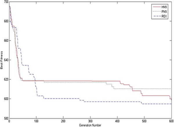

  

  Typical routes with and without waiting time.

  It must be mentioned that each route is divided to some sections (each section is named path) according to the number of trains with waiting time, and this operator is applied on each path that has one train with waiting time. This procedure is shown in Figure 14b, and according to it, the fuzzy operator is applied on paths 1 and 2.

• 2. The sum of the slope of satisfaction function at locomotive arrival time for each train on the path should be larger than zero. In this case, a possible forward push will cause the increase of total grade of satisfaction on the path.

So, this operator is applied on each path with above characteristics. In each step, the feasible forward push should be calculated, and the arrival time of each train should be pushed according to it. The feasible forward push in each step is shown below:

$$Push=min({\Delta }_i,w)\text{,}$$

(11)

where

$${\Delta }_{(i)}=\{\begin{array}{l}{u}_i-t_i{\text{\hspace{0.17em}\hspace{0.17em}\hspace{0.17em}\hspace{0.17em}if\hspace{0.17em}e}}_{\text{i}}<t_i<u_i\\ l_i-t_i{\text{\hspace{0.17em}\hspace{0.17em}\hspace{0.17em}\hspace{0.17em}\hspace{0.17em}if\hspace{0.17em}u}}_{\text{i}}<t_i<l_i\end{array}\text{.}$$

(12)

After this push, the section of path from the train^* to end of the path is considered, and the above characteristics are checked again. So, if the characteristics are okay, the new feasible forward push will be calculated, and the operator will apply on this section again. This procedure is repeated until the new feasible forward push could not be found. It must be mentioned that, the train^* is the train that the previous minimum push is found on it.

Hill climbing and recovery

Also the hill climbing is used in order to improve the chromosomes obtained through crossover and mutation. Hill climbing is a scheme for randomly selecting a portion of the population and improving them by a few iterations of removal and reinsertion. At the end, to additionally improve the quality of the population, the worst portion of the population will be replaced with the best of the parent population.

Authors' information

SN is the associate professor of Industrial Engineering Department in Iran University of Science and Technology (IUST) since October 1990. The teaching experiences are mainly in project management, human resource management, organizational behaviour and HRM, and engineering economic and preventive maintenance. SFG is a PhD student of Industrial Engineering Department in Iran University of Science and Technology (IUST). He specializes research in the field of transportation, railway engineering, vehicle routing problem, and engineering economic and preventive maintenance.

References

Ahuja RK, Liu J, Orlin JB, Sharma D, Shughart LA: Solving real-life locomotive scheduling problems. Transp Sci 2005,39(4):503–517. 10.1287/trsc.1050.0115
Alvarenga GB, Mateus GR, de Tomi G: A genetic and set partitioning two-phase approach for the vehicle routing problem with time windows. Computers & Operation Research 2007, 34: 1561–1584. 10.1016/j.cor.2005.07.025
Berger J, Barkaoui M: A hybrid genetic algorithm for the capacitated vehicle routing problem. In GECCO'03 proceedings of the 2003 international conference on genetic and evolutionary computation: Part I, Chicago, IL, USA, July 12–16, 2003. Edited by: Cantú-Paz E. Springer, Heidelberg; 2003:646–656.
Brannlund V, Lindberg PO, Nou A, Nilsson JE: Railway timetabling using Lagrangian relaxation. Transp Sci 1998,32(4):358–369. 10.1287/trsc.32.4.358
Bräysy O, Gendreau M: Metaheuristics for the vehicle routing problem with time windows. Internal Report STF42 A01025, SINTEF Applied Mathematics. Department of Optimization, Norway; 2001.
Cerda J, Dondo R: A cluster-based optimization approach for the multi-depot heterogeneous fleet vehicle routing problem with time windows. Eur J Oper Res 2007, 176: 1478–1507. 10.1016/j.ejor.2004.07.077
Cheng R, Gen M, Tozawa T: Vehicle routing problem with fuzzy due-time using genetic algorithm. Japan Society for Fuzzy Theory and System 1996,7(5):1050–1061.
Cordeau JF, Toth P, Vigo D: A survey of optimization models for train and scheduling. Transp Sci 1998,32(4):988–1005.
Cordeau JF, Soumins F, Desrosiers J: A Bender decomposition approach for the locomotive and car assignment problem. Transp Sci 2000,34(4):133–149.
Cordeau JF, Desauliniers G, Lingaya N, Soumis F, Desrosiers J: Simultaneous locomotive and car assignment at VIA Rail Canada. Transportation Research Part B 2001, 35: 767–787. 10.1016/S0191-2615(00)00022-9
Cordeau JF, Soumins F, Desrosiers J: Simultaneous assignment of locomotives and cars to passenger trains. Operation Research 2001, 49: 531–548. 10.1287/opre.49.4.531.11226
Crevier B, Cordeau JF, Laporte G: The multi-depot vehicle routing problem with inter-depot routes. Eur J Oper Res 2007, 176: 756–773. 10.1016/j.ejor.2005.08.015
Czech ZJ, Czarnas P: Parallel simulated annealing for the vehicle routing problem with time windows. In Proceeding of the 10th Euromicro workshop on parallel, distributed and network-based processing, Canary Islands, Spain, January 9, 2002. IEEE, NY, USA; 2002:376–383.
Fioole PJ, Kroon L, Maroti G, Schrijver A: A rolling stock circulation model for combining and splitting of passenger trains. European Journal of Operation Research 2006, 174: 1281–1297. 10.1016/j.ejor.2005.03.032
Florian M, Bushell G, Ferland J, Guerin G, Nastansky L: The engine scheduling problem in a railway network. Infor 1976, 14: 121–138.
Forbes MA, Holt JN, Walts AM: Exact solution of locomotive scheduling problem. Journal of the Operation Research Society 1991, 42: 825–831.
Gambardella LM, Taillard E, Agazzi G: MACS-VRPTW: A multiple ant colony system for vehicle routing problems with time windows. In New Ideas in Optimization. Edited by: Corne D, Dorigo N, Glover F. McGraw-Hill, Columbus; 1999:63–76.
Ghoseiri K, Ghannadpour SF: Locomotive routing problem using a hybrid genetic algorithm. Journal of Transportation Research 2009,5(3):259–273.
Ghoseiri K, Ghannadpour SF: Hybrid genetic algorihtm for vehicle routing and scheduling problem. Journal of Applied Science 2009,9(1):79–87. 10.3923/jas.2009.79.87
Ghoseiri K, Ghannadpour SF: A hybrid genetic algorithm for multi-depot homogenous locomotive assignment with time windows. Appl Soft Comput 2010, 10: 53–65. 10.1016/j.asoc.2009.06.004
Holland JH: Adaptation in natural and artificial system. The University of Michigan Press, Ann Arbor, MI; 1975.
Irnich S, Funke B, Grunert T: Sequential search and its application to vehicle routing problems. Computer & Operations Research 2006, 33: 2405–2429. 10.1016/j.cor.2005.02.020
Kim BI, Kim S, Sahoo S: Waste collection vehicle routing problem with time windows. Comput Oper Res 2006, 33: 3624–3642. 10.1016/j.cor.2005.02.045
Laporte G, Semet F: Classical Heuristics for the Vehicle Routing Problem. Les Cahiers du GERAD, G-98–54. Group for Research in Decision Analysis, Montreal, Canada; 1999. Accessed 06 December 2010 http://www.gerad.ca/en/publications/cahiers_rech.php?r_numero=&r_titre=Classical+Heuristics+for+the+Vehicle+Routing+Problem&r_titre_ancien=&r_auteurs=&r_journal_paru=&r_paru_mois=&r_paru_annee=&r_rev_mois=&r_rev_annee=&r_resume=&tri=num&rech=Search Accessed 06 December 2010
Li F, Golden B, Wasil E: Very large scale vehicle routing: new test problems algorithms and results. Comput Oper Res 2005, 32: 1165–1179. 10.1016/j.cor.2003.10.002
Lingaya N, Cordeau JF, Desaulniers G, Desrosiers J, Soumis F: Operational car assignment at VIA Rail Canada. Transportation Research Part B 2002, 36: 755–778. 10.1016/S0191-2615(01)00027-3
Pisinger D, Ropke S: A general heuristic for vehicle routing problem. Computer & Operations Researches 2007, 34: 2403–2435. 10.1016/j.cor.2005.09.012
Rouillon S, Desaulniers G, Soumis F: An extended branch-and-bound method for locomotive assignment. Transportation Research Part B 2006, 40: 404–423. 10.1016/j.trb.2005.05.005
Sheng HM, Wang JC, Huang HH, Yen DC: Fuzzy measure on vehicle routing problem of hospital materials. Expert Systems with Application 2006, 30: 367–377. 10.1016/j.eswa.2005.07.028
Solomon MM: Algorithms for vehicle routing problem and scheduling problems with time window constraints. Operation research 1987, 35: 254–365. 10.1287/opre.35.2.254
Tan KC, Chew YH, Lee LH: A hybrid multiobjective evolutionary algorithm for solving vehicle routing problem with time windows. Comput Optim Appl 2006, 34: 115–151. 10.1007/s10589-005-3070-3
Tan KC, Cheong CY, Goh CK: Solving multiobjective vehicle routing problem with stochastic demand via evolutionary computation. Eur J Oper Res 2007, 177: 139–813.
Vaidyanathan B, Ahuja RK, Orlin JB: The locomotive routing problem. Transp Sci 2008, 42: 492–507. 10.1287/trsc.1080.0244
Vaidyanathan B, Ahuja RK, Liu J, Shughart LA: Real-life locomotive planning: New formulations and computational results. Transportation Research Part B: Methodological 2008, 42: 147–168. 10.1016/j.trb.2007.06.003
Ziarati K, Soumis F, Desrosiers J, Gelinas S, Saintonge A: Locomotive assignment with heterogeneous consists at CN North America. European Journal of Operation Research 1997, 97: 281–292. 10.1016/S0377-2217(96)00198-1
Acknowledgments
The authors would like to acknowledge and thank the editors and reviewers of this manuscript that their valuable input and correspondences helped this manuscript to improve.
Author information
Authors and Affiliations
Corresponding author
Additional information
Competing interests
Both authors declare that they have no competing interests.
Authors' contributions
SN conceived of the study and participated in its design and coordination. SFG participated in the design of the study and performed the statistical analysis. All authors read and approved the final manuscript.
Authors’ original submitted files for images
Below are the links to the authors’ original submitted files for images.
Rights and permissions
Open Access This article is distributed under the terms of the Creative Commons Attribution 2.0 International License (https://creativecommons.org/licenses/by/2.0), which permits unrestricted use, distribution, and reproduction in any medium, provided the original work is properly cited.
About this article
Cite this article
Noori, S., Ghannadpour, S.F. Locomotive assignment problem with train precedence using genetic algorithm. J Ind Eng Int 8, 9 (2012). https://doi.org/10.1186/2251-712X-8-9
Received:
Accepted:
Published:
DOI: https://doi.org/10.1186/2251-712X-8-9