
Abstract
In this review article, we propose to use the Bayesian inference approach for inverse problems in signal and image processing, where we want to infer on sparse signals or images. The sparsity may be directly on the original space or in a transformed space. Here, we consider it directly on the original space (impulsive signals). To enforce the sparsity, we consider the probabilistic models and try to give an exhaustive list of such prior models and try to classify them. These models are either heavy tailed (generalized Gaussian, symmetric Weibull, Student-t or Cauchy, elastic net, generalized hyperbolic and Dirichlet) or mixture models (mixture of Gaussians, Bernoulli-Gaussian, Bernoulli-Gamma, mixture of translated Gaussians, mixture of multinomial, etc.). Depending on the prior model selected, the Bayesian computations (optimization for the joint maximum a posteriori (MAP) estimate or MCMC or variational Bayes approximations (VBA) for posterior means (PM) or complete density estimation) may become more complex. We propose these models, discuss on different possible Bayesian estimators, drive the corresponding appropriate algorithms, and discuss on their corresponding relative complexities and performances.
1 Introduction
In many generic inverse problems in signal and image processing we want to infer on an unknown signal f(t) or an unknown image f(r) with r= (x, y) through an observed signal g(s) or an observed image g(s) related between them through an operator such as convolution g = h * f or any other linear or non linear transformation . When this relation is linear and we have discretized the problem, we arrive to the relation:
where f= [f1, ..., f n ]' represents the unknowns, g= [g1, ..., g m ]' the observed data, ϵ= [ϵ1, ..., ϵ m ]' the errors of modeling and measurement and H the matrix of the system response. We may note that, even if the noise could be neglected (ϵ= 0) and the matrix H invertible (m = n), in general, the solution is not forcibly the good solution, because this solution may be too sensitive to small changes in the data due to the ill-conditioning of this matrix. for the general case of m ≠ n, one tries to obtain a regularized solution, for example by defining it as the optimizer of a two parts criterion
which is given by . When the regularization parameter λ = 0, one gets a generalized inverse and when H invertible, one gets the normal inverse solution . The regularization theory has been developed since the pioneer work of Tikhonov [1] and Tikhonov and Arsénine [2] who had introduced a quadratic regularization terms to account for some prior properties of the solution (smoothness). Since that, many different regularization terms have been proposed. In particular, in place of L2 norm: , it has been proposed to use the L0 norm or the L1 norm L1(f) = ||f||1 = Σ j |f j | to enforce the sparsity of the solution [3–11]. Then, due to the fact that L0(f) is not convex and L1(f) is convex, but not continuous, the optimization of a criterion with these expressions becomes more difficult than the L2 norm case. For this reason, there was a great number of works who specialized in proposing algorithms for the optimization of such criteria.
Interestingly, defining the solution of the problem (1) as the optimization of a criterion with two parts can be assimilated to a maximum a posteriori (MAP) solution in a Bayesian approach where the first term of the criterion (2) can be related to the likelihood and the second term to a prior model as we will see in the following where the main objective is to show how the Bayesian approach can go farther than the regularization in at least the following aspects:
-
A better account for the noise term characteristics;
-
A better and easier way for translating the prior knowledge and in particular the sparsity;
-
New tools for assessing the regularization parameter, a great subject of discussion for all those work with regularization theory;
-
New solutions and new tools for doing computations (optimizations and integrations).
1.1 The Bayesian approach
The Bayesian inference approach is based on the posterior law:
where the sign ∝ stands for "proportional to", p(g|f, θ1) is the likelihood, p(f|θ2) the prior model, θ= (θ1, θ2) are their corresponding parameters (often called the hyper parameters of the problem) and p(g|θ1, θ2) is called the evidence of the model.
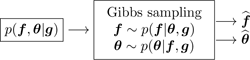
This general Bayesian approach is illustrated as follows:

In this approach, the likelihood p(g|f, θ1) summarizes our knowledge about the noise and the model linking the observed data g to the unknowns f and the prior term p(f|θ2) summarizes our incomplete prior knowledge about the unknowns and the posterior law p(f|g, θ) combines these two terms and contains all our state of knowledge about the unknowns f after accounting for the prior and the observed data.
As a very simple example, when the noise is assumed to be Gaussian, then the MAP solution is obtained as the optimizer of the criterion J(f) = ||g- Hf||2 + λ Ω(f) where the expression of Ω(f) depends on the prior law. When the prior knowledge is translated as a Gaussian probability law, then and when it is translated as a Laplace probability law, then Ω(f) = ||f||1 [12–14].
The first interest of using the Bayesian approach to the regularization approach is to have new tools for handling the hyper parameters [15].
1.2 Full Bayesian approach
When the parameters θ have to be estimated too, we can assign them a prior p(θ|θ0) with fixed values for θ0 (often called hyper-hyper-parameters) and express the joint posterior
and then try to estimate them jointly, for example joint MAP [16]:
This Full Bayesian approach is illustrated as follows:

One may also first integrate out one of them, for example f to obtain
estimate θ, for example by
and then use it for the estimation of the other one using .
This approach (called sometimes type II maximum likelihood) is illustrated as follows:

However, very often this marginalization cannot be done analytically and so the optimization for the estimation of θ cannot be achieved. In such cases, the expectation-maximization (EM) algorithms can be helpful [17]. Considering g as incomplete data, f as hidden variable, (g, f) as complete data and noting ln p(g|θ) as incomplete data log-likelihood and ln p(g, f|θ) complete data log-likelihood, the classical EM algorithm writes:
The Bayesian version (Bayesian EM) is not very far and differs only by the introduction of p(θ):
This is illustrated as follows:

As we mentioned before, one of the main steps in the Bayesian approach is the prior modeling which has the role of translating our prior knowledge on the unknown signal or image in a probability law. Sparsity is one of the prior knowledge we may translate. The main objective of this article is to see what are the different possibilities.
1.3 Prior modeling
In this article, we propose different prior modeling for signals and images which can be used in a Bayesian inference approach in many inverse problems in signal and image processing where we want to infer on sparse signals or images. The sparsity may be directly on the original space or in a transformed space (see Figures 1, 2, 3, and 4). In this article, we consider the sparsity directly in the original domain.

Sparsity: explicite sparse signals. The signal at the right is sparse, but its derivative (signal at the left) is still more sparse.

Sparsity: sparse signals in a transformed domaine (Fourier or wavelet). First row: signals, second row: Fourier or wavelet transforms.

Sparsity: explicite sparse images. The images at the top are sparse. The images at the bottom are not sparse, but their Laplaciens are (images at top).

Sparsity: sparse images in a transformed domain (Fourier or wavelet). First row: images, second row: Fourier or wavelet transforms.
The prior models discussed are the following:
-
generalized Gaussian (GG) with Gaussian (G) and Laplace or double exponential (DE) as particular cases;
-
symmetric Weibull (W) with symmetric Rayleigh (R) and again the DE as particular cases;
-
Student-t (St) with Cauchy (C) as particular case;
-
Elastic net prior model;
-
generalized hyperbolic model;
-
Dirichlet and symmetric Dirichlet;
-
Mixture of two centered Gaussians (MoG2), one with very small and one with a large variances;
-
Bernoulli-Gaussian (BG), also called Spike and slab;
-
Mixture of two Gammas (MoGamm);
-
Bernoulli-Gamma (BGamma);
-
Mixture of three Gaussians (MoG3), one centered with very small variance and two symmetrically centered on positive and negative axes and large variances;
-
Mixture of one Gaussian and two Gammas (MoGGammas), and in a more summary the case of
-
Bernoulli-Multinomial (BMult) or mixture of Dirichlet (MoD).
Some of these models are well-known [12–14, 18–26], some others less. In general, we can classify them into two categories: (i) simple non Gaussian models with heavy tails and (ii) mixture models with hidden variables which result to hierarchical models.
In the Section 2, we give more details about the sparsity and all these prior models which enforce the sparsity.
1.4 Bayesian computation
The second main step in the Bayesian approach is to do the computations. Depending on the prior model selected, the Bayesian computations needed are:
-
For simple prior models:
-
Simple optimization of p(f|θ, g) for the MAP:

-
Joint optimization p(f, θ|g) for joint MAP:

-
Generation of samples from the conditionals p(f|θ, g) and p(θ|f, g) for the MCMC Gibbs sampling methods,
-
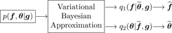
Variational approximation (VA) of the joint p(f, θ|g) by a separable
and then using them for estimation
-


-
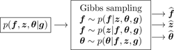
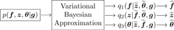
For hierarchical prior models with hidden variables z:
-
Joint optimization p(f, z, θ|g) for joint MAP,

-
Generation of samples from the conditionals p(f|z, θ, g), p(θ|z, f, g) and p(z|f, θ, g) for the MCMC Gibbs sampling methods:
-
Variational approximation (VA) of the joint p(f, z, θ|g) by a separable
and then using them for estimation
-


The second main objective of this article is to discuss on the relative complexities and performances of the algorithms obtained with the proposed prior law.
The rest of the article is organized as follows:
In Section 2, we present in details the proposed prior models and discuss their properties. For example, we will see that the Student-t model can be interpreted as an infinite mixture with a variance hidden variable or that the BG model can be considered as the degenerate case of a MoG2 where one of the variances go to zero. Also, we will examine the less known models of MoG3 and MoGGammas where the heavy tails are obtained by combining a centered Gaussian and two large variance non-centered Gaussians or Gammas.
In Section 3, we examine the expression of the posterior laws that we obtain using these priors and discuss then on complexity of the Bayesian computation of the algorithms. In particular for the mixture models, we give details of the joint estimation of the signal and the hidden variable as well as the hyper parameters (parameters of the mixtures and the noise) for unsupervised cases.
In Section 4, we give more details on the variational Bayesian approximation method, first for the general case and then for the case of mixture laws and more specifically the case of the Student-t considered as a continuous mixture.
Finally, we present the main conclusions of this article in Section 5.
2 Prior models enforcing sparsity
First, as we mentioned, the sparsity is a property which can be described either directly for the signal itself or after some transformation, for example on the derivative of the signal, or in more general on the coefficients of the projection of the signal on any basis or any set of functions.
Different prior models have been used to enforce sparsity.
2.1 Generalized Gaussian (GG), Gaussian (G) and double exponentials (DE) models
This is the simplest and the most used model (see for example, [27]). Its expression is:
where
Two particular cases are of importance:
-
β = 2 (Gaussian):
(12) -
β = 1 (double exponential or Laplace):
(13)
The general shape of these priors are shown in Figure 5, where the cases β = 1 and 0 < β < 1, which are of great interest for sparsity enforcing are compared to the Gaussian case β = 2.

Generalized Gaussian family. The probability density function p(x) is shown in the left and - ln p(x) is shown in the right.
2.2 Symmetric Weibull (W) and symmetric Rayleigh (R) models
The second model we consider is the symmetric Weibull probability density function (pdf):
where
and where γ > 0 and β > 0, and the particular cases of β = 1 is the double exponential and β = 2 is the symmetric Rayleigh distribution:
the cases where 0 < β < 1 are of great interest for sparsity enforcing. This family of models are illustrated on Figure 6.

Symmetric Weibull family. The probability density function p(x) is shown in the left and - ln p(x) is shown in the right.
2.3 Student-t (St) and Cauchy (C) models
The second simplest model is the Student-t model:
where
Knowing that
we can write this model via the positive hidden variables τ j :
Cauchy model is obtained when ν = 1:
This family of models are illustrated on Figure 7.

Student-t and Cauchy family. The probability density function p(x) is shown in the left and - ln p(x) is shown in the right.
2.4 Elastic Net (EN) prior model
A prior model inspired from elastic net regression literature [28] is:
where
which is a product of a Gaussian and a double exponential pdfs. This family of models are illustrated on Figure 8.

Elastic net family. The probability density function p(x) is shown in the left and - ln p(x) is shown in the right.
2.5 Generalized hyperbolic (GH) prior model
Another general prior model which can be used is:
where Kν-1/2is the second kind Bessel function of order (ν - 1/2). This family of models are illustrated on Figure 9.

Generalized hyperbolic family. The probability density function p(x) is shown in the left and - ln p(x) is shown in the right.
2.6 Dirichlet (D) and symmetric Dirichlet (SD) models
When f j are positive and sums to one, we can use the Dirichlet model
where α= {α1, ..., α N } with α j > 0. The proportionality constant is
It is noted that the support of this distribution is [0,1]Nand ||f||1 = Σ j f j = 1.
It is also interesting to note that the domain of the Dirichlet distribution is itself a probability distribution, specifically a N-dimensional discrete distribution and the set of points in the support of a N-dimensional Dirichlet distribution is the open standard N - 1-simplex, which is a generalization of a triangle, embedded in the next-higher dimension.
A very common special case is the symmetric Dirichlet (SD) distribution, where all of the elements making up the parameter vector α have the same value α called the concentration parameter:
When α > 1, the symmetric Dirichlet distribution is equivalent to a uniform distribution over the open standard standard N - 1-simplex, i.e., it is uniform over all points in its support. α > 1 prefer variants that are dense, evenly-distributed distributions, i.e., all probabilities f j returned are similar to each other. α < 1 prefer sparse distributions, i.e., most of the probabilities f j returned will be close to 0, and the vast majority of the mass will be concentrated in a few of them. This is the case on which we are interested. An illustration of this family of models are illustrated on Figure 10.

Dirichlet family. The probability density function p(x) is shown in the left and - ln p(x) is shown in the right.
2.7 Mixture of two Gaussians (MoG2) model
The mixture models are also very commonly used as prior models. In particular the mixture of two Gaussians (MoG2) model:
which can also be expressed through the binary valued hidden variables z j ∈ {0,1}
In general v1 >> v0 and λ measures the sparsity (0 < λ << 1). This family of models are illustrated on Figure 11.

Mixture of two Gaussians family. The probability density function p(x) is shown in the left and - ln p(x) is shown in the right.
2.8 Bernoulli-Gaussian (BG) model
The Bernoulli-Gaussian model can be considered as the particular case of the MoG2 with the particular degenerate case of v0 = 0:
which can also be written as
This model has also been called spike and slab. This family of models are illustrated on Figure 12.

Bernouilli-Gaussian family. The probability density function p(x) is shown in the left and - ln p(x) is shown in the right.
2.9 Mixture of three Gaussians (MoG3) model
Another mixture model proposed is using a Mixture of three Gaussians, one centered at zero and two symmetrically placed:
which can also be expressed through the ternary valued hidden variables z j ∈ {-1, 0, +1}
In general v+1 = v-1 = v >> v0 and λ measures the sparsity (0 < λ << 1). This family of models are illustrated on Figure 13.

Mixture of three Gaussians family. The probability density function p(x) is shown in the left and - ln p(x) is shown in the right.
2.10 Mixture of one Gaussian and two Gammas (MoGGammas) model
Another mixture model proposed is using a mixture of one central Gaussian and two symmetric Gammas:
which can also be expressed through the ternary valued hidden variables z j ∈ {-1, 0, +1}
This family of models are illustrated on Figure 14.

Mixture of one Gaussian and two Gammas family. The probability density function p(x) is shown in the left and - lnp(x) is shown in the right.
2.11 Bernoulli-Gamma (BGamma) model
As in the BG model, when we want to enforce both sparsity and positivity, we can use the BGamma model:
or
A particular case of this model is Bernoulli-exponential (BExponential) which obtained when α = 1. These families of models are illustrated on Figure 15 and Figure 16.

Bernouilli-Gamma family. The probability density function p(x) is shown in the left and - ln p(x) is shown in the right.

Mixture of 2 Gammas family. The probability density function p(x) is shown in the left and - ln p(x) is shown in the right.
2.12 Mixture of Dirichlet (MoD) model
-
Mixture of Dirichlet model
(38)
where
is the symmetric Dirichlet distribution. We need to choose α1 > 1 for dense part and 0 < α2 < 1 for the sparse part.
2.13 Bernoulli-multinomial (BMultinomial) model
As in the BG or BGamma model, when we know that the signal is sparse and can only take one of the K discrete values {a1, ..., a K }, we can use the BMultinomial model:
where a= {a1, ..., a K } and α= {α1, ..., α K } with ∑ k α k = 1 and
or
3 Bayesian inference with sparsity enforcing priors
The priors proposed can be used in a Bayesian approach to infer on f given the observed data g through the posterior law given in Equation (3). First let assume the error ϵ to be centered, Gaussian and white: . Then, using the forward model (1) we have
Now, we consider different priors.
3.1 Simple prior models
Given p(g|f) and any simple prior law p(f), the posterior law is written:
with
where Ω(f) = -ln p(f) and so the Maximum A Posteriori (MAP) solution is expressed as the minimizer of this criterion which has two parts: the first part is due to the likelihood and the second part is due to the prior:

Thus, depending on the choice of the prior we obtain different expressions for Ω(f). For example for the GG model of (10) we get
For the symmetric Weibull model (14) we get
For the Student-t model (17) we get
For the elastic net model we get
and for the Dirichlet model we get
For each of these cases, we may discuss on the unimodality and convexity of the criterion J(f) which depends mainly on its Hessian
We may look at each case to examine the range of the parameters for which this Hessian matrix is positive definite.
The optimization is done iteratively:

Update operation can be additive, multiplicative or more complex. Updating steps α(k)can be fixed or computed adaptively at each step (steepest descent for example). δ f(k)can be, for example proportional to the gradient, in which case, we have

We may also consider to estimate some of these parameters by assigning them appropriate priors and then express the joint p(f, θ|g, θ0) as given in Equation (4) and then try to estimate them jointly, for example joint MAP:

or alternate optimization:

We may also want to explore this joint posterior by generating samples from it. This can be done, for example, through the following Gibbs sampling scheme:

When a great number of samples are thus generated, we may compute their means, variances or any other statistics about them.
Finally, we may try to approximate this joint posterior by a simpler one, for example by a separable q(f, θ) = q1(f) q2(θ) using the variational approximation (VA). The main idea and the main basic steps to achieve this is more detailed in the following section. Here, however, we present the result on the following scheme:

To illustrate the differences, we may consider the simple case of a linear forward model and Gaussian priors:
In this case, if we know θ= (v ϵ , v f ), then
with . So, we have which can be computed by optimizing J(f) = ||g- H f||2 + λ||f||2. A gradient based algorithm is shown below:

Now putting inverse Gamma priors on v ϵ and v f , or equivalently Gamma priors on τ ϵ = 1/v ϵ and τ f = 1/v f :
we have
with
and . Then, the alternate optimization of the JMAP estimate algorithm becomes

The Gibbs sampling algorithm becomes

The VBA algorithm becomes
and :

We recently implemented these algorithms for different applications such as: synthetic aperture radar (SAR) Imaging [29], ...
3.2 Mixture models
For the mixture models, and in general for the models which can be expressed via the hidden variables, we want to estimate jointly the original unknowns f and the hidden variables: τ in Cauchy model, z in MoG2, BG or BGam models and z in MoG3 or MoGGammas. Let examine these a little in details.
3.3 Student-t and Cauchy models
In this case the joint prior law can be written as:
such that
where

Joint optimization of this criterion, alternatively with respect to f(with fixed τ)
and with respect to τ(with fixed f)
results in the following iterative algorithm:

Note that, τ j is the inverse of a variance and we have . We can interpret this as an iterative quadratic regularization inversion followed by the estimation of variances τ j which are used in the next iteration to define the variance matrix D(τ).
Here too, we may study the conditions on which the joint criterion is uni-modal and its alternate optimization converges to its unique solution.
We may also consider a Gibbs sampling scheme
where
and

For the VBA, we have

3.4 Mixture of two Gaussians (MoG2) model
In this case, following the same arguments, we obtain:
where
Again, in this case also, the optimization of this criterion, alternatively with respect to f and z results in the following iterative algorithm:

Here too, we may also consider a Gibbs sampling scheme
where
and

3.5 BG model
For the case of BG we have to be more careful, because the joint probability laws are degenerated. Two approaches are then possible:
i) Considering them as the particular case of the MoG models where the variance v0 is fixed to a small value or reduced gradually during the iterations.
ii) Trying first to integrate out f from the expression of p(f, z|g) to obtain p(z|g) and optimize it with respect to z(detection step) and then use it for the estimation step.
To go further in detail of the second approach, we may remark that for the given z, the expression of p(f, z|g) as a function of f is Gaussian and so it can be easily integrated out and we obtain:
Now writing the expression of and keeping only all terms depending on z we obtain:
where B(z) = H(v diag [z j , j = 1, ..., n])H' + v ϵ I. We see the complexity of this expression which needs the inversion of the matrix B and its optimization which is a combinatorial optimization needing to evaluate this expression 2ntimes.
However, we may also remark that when z obtained, the estimation of f is easy. We have:
which needs again the inversion of the matrix B.
The exact computations of and are often too costly, one may try to obtain approximate solutions. Many approximations have been proposed. A good overview of these methods can be found in [30, Chap. 5] and also in [31, 32].
3.6 BGamma and MoGGammas model
In these cases, it is no more possible to integrate out f analytically as it was the case with Gaussians. One strategy here is to use the MCMC methods to generate samples from the joint posterior. The second approach is to approximate the joint posterior by a simpler one, for example by a separable one on f and the hidden variables z in the BGamma or the MoGGammas cases. Very often then we can do the computations analytically. However, it may happens that, even after these separable approximations, still we need to use the MCMC methods on some of variables. Detailed explanation of these general methods is out of focus of this article. See [30, 33, 34]. Here, we just give the details for the case of the Gaussian mixtures (MoG2 or MoG3).
4 Variational Bayesian approximation for the case of mixture laws
To start and to be complete as to propose an unsupervised method, we include also the estimation of the parameters θ and write the joint posterior law of all the unknowns:
which can also be written as
where
with
and
with
or
when z are discrete valued, and finally
with
One can also write:
and
or
when z are discrete valued.
We see that the first term
will be easy to handle because it is the product of two Gaussians and so it is a multivariate Gaussian. But the two others are not.
The main idea behind the VBA is to approximate the joint posterior p(f, z, θ|g) by a separable one, for example
illustrated here:

and where the expressions of q(f, z, θ|g) is obtained by minimizing the Kullback-Leibler divergence
It is then easy to show that
where is the likelihood of the model
with
and is the free energy associated to q defined as
So, for a given model , minimizing KL(q : p) is equivalent to maximizing and when optimized, gives a lower bound for .
Without any other constraint than the normalization of q, an alternate optimization of with respect to q1, q2, and q3 results in
Note that these relations represent an implicit solution for q1(f), q2(z), and q3(θ) which need, at each iteration, the expression of the expectations in the right hand of exponentials. If p(g|f, z, θ1) is a member of an exponential family and if all the priors p(f|z, θ2), p(z|θ3), p(θ1), p(θ2), and p(θ3) are conjugate priors, then it is to see that these expressions leads to standard distributions for which the required expectations are easily evaluated. In that case, we may note
where the tilded quantities and are, respectively functions of and :

and where the alternate optimization results to alternate updating of the parameters for q1, the parameters of q2 and the parameters of q3.

Finally, we may note that, to monitor the convergence of the algorithm, we may evaluate the free energy
where all the expectations are with respect to q.
Other decompositions are also possible:
illustrated here:

or even by:
illustrated here:

Here, we consider the second case (Equation (95)) and give some more details on it. First to simplify the notations, we write it as:
where it can be shown that:
where p(f, z, θ, g) = p(g|f, θ)p(f|z, θ)p(z|θ)p(θ) and where q2(z) = Π j q2j(z j ), q3(θ) = Π l q3l(θ l ), q2(z(-j)) = Πi≠jq2j(z j ), 〈.〉 q means expected value with respect to q.
In that case, with appropriate models for the priors (exponential families) and hyper parameters (conjugate priors), we see that q(f) is a multivariate Gaussian , q(θ l ) are either Gaussians (for the means) or Inverse Gammas (for the variances) and q(z j ) are discrete distributions whose expressions can be written easily.
To illustrate this in more detail, we consider the case of the Student-t model.
4.1 Student-t model
In this case, we have the following relations for the forward model and the prior laws:
Then, we obtain the following expressions for the VBA:
where the expressions of the expectations needed are:
We can also express the free energy expression:
where
and
In these equations,
The resulting algorithm can be summarized as follows

5 Conclusion
The sparsity is a required property in many signal and image processing applications. In this article, first we reviewed the main steps of the Bayesian approach for inverse problems in signal and image processing. Then we presented in a synthetic way the different prior models which can be used to enforce the sparsity. These models have been presented in two categories: simple and hierarchical with hidden variables. For each of these prior models, we discuss their properties and the way to use them in a Bayesian approach resulting to many different inversion algorithms.
We have applied these Bayesian algorithms in many different applications such as X-ray computed tomography [35, 36], optical diffraction tomography [37–39], positron emission tomography [40], Microwave imaging [41, 42], Sources separation [43–46], spectrometry [47, 48], Hyper spectral imaging [49], super resolution [50–52], image fusion [53], image segmentation [54], synthetic aperture radar (SAR) imaging [29]. To save the place and be very synthetic, we did not give here any simulation results or any results on different applications of these methods. These can be found in different articles just referenced.
References
Tikhonov A: Regularization of incorrectly posed problems. Soviet Math Dokl 1963, 4: 1624-1627.
Tikhonov A, Arénine V: Méthodes de Résolution de Problémes Mal Posés. MIR, Moscu, Russia; 1976. Éditions
Daubechies I, Defrise M, Mol CD: An iterative thresholding algorithm for linear inverse problems with a sparsity constraint. Comm Pure Appl Math 2004, 57: 1413-1457. 10.1002/cpa.20042
Donoho DL: Compressive sampling. IEEE Trans Inf Theory 2006, 52(4):1289-1306.
Tropp JA, Gilbert AC, Strauss MJ: Algorithms for simultaneous sparse approximation. Part I: Greedy pursuit. Signal Processing, special issue "sparse approximations in signal and image processing" 2006, 86: 572-588.
Tropp JA: Algorithms for simultaneous sparse approximation. Part II: Convex relaxation. Signal Process (special issue "Sparse approximations in signal and image processing") 2006, 86: 589-602.
Zass R, Shashua A: Nonnegative Sparse PCA. Volume 19. Cambridge, MA: MIT Press; 2007:1561-1568.
Candés EJ, Wakin M, Boyd S: Enhancing sparsity by reweighted l1 minimization. J Fourier Anal Appl 2008, 14: 877-905. 10.1007/s00041-008-9045-x
Witten DM, Tibshirani R, Hastie T: A penalized matrix decomposition, with applications to sparse principal components and canonical correlation analysis. Biostatistics 2009, 10(3):515-534. 10.1093/biostatistics/kxp008
Vaiter S, Peyré G, Dossal C, Fadili J: Robust Sparse Analysis Reg-ularization. Tech rep, preprint Hal-00627452 2011. [http://hal.archives-ouvertes.fr/hal-00627452/]
Peyré G, Fadili J: Learning Analysis Sparsity Priors. Proc of Sampta'11 2011. [http://hal.archives-ouvertes.fr/hal-00542016/]
Williams P: Bayesian regularization and pruning using a Laplace prior. Neural Comput 1995, 71: 117-143.
Mitchell T, Beauchamp J: Bayesian variable selection in linear regression. J Am Stat Assoc 1988, 83(404):1023. 10.2307/2290129
Polson N, Scott J: Shrink globally, act locally: sparse Bayesian regulariza-tion and prediction. Bayesian Stat 2010, 9: 1-24.
Mohammad-Djafari A: On the estimation of hyperparameters in Bayesian approach of solving inverse problems. In Proc IEEE International Conference on Acoustics, Speech, and Signal Processing ICASSP-93. Volume 5. Minneapolis, MN, USA; 1993:495-498.
Mohammad-Djafari A: Joint estimation of parameters and hyperparameters in a Bayesian approach of solving inverse problems. In IEEE Int Conf on Image Processing (ICIP), IEEE ICIP 96. Volume II. Lausanne, Swisse; 1996:473-477.
Neal R, Hinton G: A view of the EM algorithm that justifies incremental, sparse, and other variants. Learn Graph Models 1998, 89: 355-368.
Doucet A, Duvaut P: Bayesian estimation of state-space models applied to deconvolution of Bernoulli-Gaussian processes. Signal Process 1997, 57(2):147-161. 10.1016/S0165-1684(96)00192-2
Park T, Casella G: The Bayesian Lasso. J Am Stat Assoc 2008, 103(482):681-686. 10.1198/016214508000000337
Tipping M: Sparse Bayesian learning and the relevance vector machine. J Mach Learn Res 2001, 1: 211-244.
Févotte C, Godsill S: A Bayesian aproach for blind separation of sparse source. IEEE Trans Audio Speech Lang Process 2006, 14: 2174-2188.
Caron F, Doucet A: Sparse Bayesian nonparametric regression. International Conference on Machine Learning 2008, 88-95.
Griffin J, Brown P: Inference with normal-gamma prior distributions in regression problems. Bayesian Anal 2010, 5: 171-188.
Snoussi H, Idier J: Bayesian blind separation of generalized hyperbolic processes in noisy and underdeterminate mixtures. IEEE Trans Signal Process 2006, 54: 3257-3269.
Ishwaran H, Rao JS: Spike and slab variable selection: frequentist and Bayesian strategies. Ann Stat 2005, 33(2):730-733. 10.1214/009053604000001147
Chatzis S, Varvarigou T: Factor analysis latent subspace modeling and robust fuzzy clustering using t-distributionsclassification of binary random patterns. IEEE Trans Fuzzy Syst 2009, 17: 505-517.
Bouman CA, Sauer KD: A generalized Gaussian image model for edge-preserving MAP estimation. IEEE Trans Image Process 1993, 2(3):296-310. 10.1109/83.236536
Zou H, Hastie T: Regularization and variable selection via the elastic net. J Royal Stat Soc, Ser, B 2005, 67(2):301-320. 10.1111/j.1467-9868.2005.00503.x
Zhu S, Mohammad-Djafari A, Wang H, Deng B, Li X, Mao J: Parameter estimation for SAR micromotion target based on sparse signal representation. Eurasip special issue "Sparse approximations in signal and image processing" 2012., 13:
Idier J: Approche Bayésienne Pour les Problémes Inverses. Traité IC2, Série traitement du signal et de l'image, Hermés, Paris; 2001.
Champagnat F, Goussard Y, Idier J: Unsupervised deconvolution of sparse spike trains using stochastic approximation. IEEE Trans Signal Process 1996, 44(12):2988-2998. 10.1109/78.553473
Ge D, Idier J, Le Carpentier E: A new MCMC algorithm for blind Bernoulli-Gaussian deconvolution. In Proceedings of EUSIPCO: Septembre 2008. Lausanne, Suisse; 2008.
Kormylo JJ, Mendel JM: Maximum-likelihood detection and estimation of Bernoulli-Gaussian processes. IEEE Trans Inf Theory 1982, 28: 482-488. 10.1109/TIT.1982.1056496
Lavielle M: Bayesian deconvolution of Bernoulli-Gaussian processes. Signal Process. 1993, 33: 67-79.
Mohammad-Djafari A: Gauss-Markov-Potts priors for images in computer tomography resulting to joint optimal reconstruction and segmentation. Int J Tomography Stat 2008, 11(W09):76-92. [http://djafari.free.fr/pdf/IJTS08.pdf]
Gac N, Vabre A: A Mohammad-Djafari, F Buyens, GPU implementation of a 3D bayesian CT algorithm and its application on real foam reconstruction. In Proceedings of the first International Conference on Image Formation in X-Ray Computed Tomography. Salt Lake City, Utah, USA; 2010.
Ayasso H, Duchne B: A Mohammad-Djafari, Bayesian inversion for optical diffraction tomography. J Modern Opt 2010, 57(9):765-776. 10.1080/09500340903564702
Ayasso H, Mohammad-Djafari A: Joint NDT image restoration and segmentation using Gauss-Markov-Potts prior models and variational Bayesian computation. IEEE Trans. Image Process 2010, 19(9):2265-2277. [http://dx.doi.org/10.1109/TIP.2010.2047902]
Ayasso H, Duchne B, Mohammad-Djafari A: Optical diffraction tomography within a variational Bayesian framework. Inverse Probl Sci Eng 2011, iFirst: 1-15.
Fall MD, Barat É, Comtat C, Dautremer T, Montagu T, Mohammad-Djafari A: A discrete-continuous Bayesian model for emission tomography. In IEEE International Conference on Image Processing (ICIP). Bruxell, Belgium; 2011:1401-1404.
Féron O, Duchêne B, Mohammad-Djafari A: Microwave imaging of inho-mogeneous objects made of a finite number of dielectric and conductive materials from experimental data. Inverse Probl 2005, 21(6):95-115. [http://djafari.free.fr/pdf/] 10.1088/0266-5611/21/6/S08
Féron O, Duchêne B, Mohammad-Djafari A: Microwave imaging of piece-wise constant objects in a 2D-TE configuration. Int J Appl Electromag Mech 2007, 26(6):167-174. [http://djafari.free.fr/pdf/jae00905.pdf]
Snoussi H, Mohammad-Djafari A: Fast joint separation and segmentation of mixed images. J Electron Imag 2004, 13(2):349-361. [http://djafari.free.fr/pdf/] 10.1117/1.1666873
Snoussi H, Mohammad-Djafari A: Bayesian unsupervised learning for source separation with mixture of Gaussians prior. J VLSI Signal Process Syst 2004, 37(2/3):263-279. [http://djafari.free.fr/pdf/VLSIpapar.pdf]
Mohammad-Djafari A: Bayesian source separation: beyond PCA and ICA. ESANN 2006 Belgium; 2006. [http://djafari.free.fr/pdf/]
Ichir M, Mohammad-Djafari A: Hidden Markov models for wavelet-based blind source separation. IEEE Trans Image Process 2006, 15(7):1887-1899.
Mohammad-Djafari A, Giovannelli J, Demoment G, Idier J: Regulariza-tion, maximum entropy and probabilistic methods in mass spectrometry data processing problems. Int J Mass Spectrom 2002, 215(1-3):175-193. [http://djafari.free.fr/pdf/maspec12013.pdf] 10.1016/S1387-3806(01)00562-0
Moussaoui S, Brie D, Mohammad-Djafari A, Carteret C: Separation of non-negative mixture of non-negative sources using a Bayesian approach and MCMC sampling. IEEE Trans Signal Process 2006, 54(11):4133-4145.
Bali N, Mohammad-Djafari A: Bayesian approach with hidden Markov modeling and mean field approximation for hyperspectral data analysis. IEEE Trans Image Process 2008, 17(2):217-225.
Humblot F, Mohammad-Djafari A: Super-resolution using hidden Markov model and bayesian detection estimation framework. EURASIP J Appl Signal Process Special number on Super-Resolution Imaging: Analysis, Algorithms, and Applications; 2006., 16: Article ID 36971 [http://www.hindawi.com/GetArticle.aspx?doi=10.1155/ASP/2006/36971]
Mohammad-Djafari A: Super-resolution: a short review, a new method based on hidden Markov modeling of HR image and future challenges. Comput J 2008. [http://djafari.free.fr/pdf/bxn005v1.pdf]
Mansouri M, Mohammad-Djafari A: Joint super-resolution and segmentation from a set of low resolution images using a Bayesian approach with a Gauss-Markov-Potts prior. Int J Signal Imag Syst Eng 2010, 3(4):211-221. 10.1504/IJSISE.2010.038017
Féron O, Mohammad-Djafari A: Image fusion and joint segmentation using an MCMC algorithm. J Electron Imag 2005., 14(2): paper no. 023014 [http://arxiv.org/abs/physics/0403150]
Brault P, Mohammad-Djafari A: Unsupervised Bayesian wavelet domain segmentation using a Potts-Markov random field modeling. J Electron Imag 2005., 14(4): 043011-1-043011-16 [http://djafari.free.fr/pdf/]
Acknowledgements
This study had been partially founded by the C5Sys project (Circadian and Cell cycle Clock systems in Cancer) of ERASYSBIO+. http://www.erasysbio.net/index.php?index=272
Author information
Authors and Affiliations
Corresponding author
Additional information
Competing interests
The author declares that they have no competing interests.
Authors’ original submitted files for images
Below are the links to the authors’ original submitted files for images.
Rights and permissions
Open Access This article is distributed under the terms of the Creative Commons Attribution 2.0 International License (https://creativecommons.org/licenses/by/2.0), which permits unrestricted use, distribution, and reproduction in any medium, provided the original work is properly cited.
About this article
Cite this article
Mohammad-Djafari, A. Bayesian approach with prior models which enforce sparsity in signal and image processing. EURASIP J. Adv. Signal Process. 2012, 52 (2012). https://doi.org/10.1186/1687-6180-2012-52
Received:
Accepted:
Published:
DOI: https://doi.org/10.1186/1687-6180-2012-52