Regularity criterion for a weak solution to the three-dimensional magneto-micropolar fluid equations

Abstract

In this paper, a regularity criterion for the 3D magneto-micropolar fluid equations is investigated. A sufficient condition on the derivative of the velocity field in one direction is obtained. More precisely, we prove that if $u_{x_3}$ belongs to $L^{\beta }(0,T;L^{\alpha }({\mathbb{R}}^3))$ with $\frac{3}{\alpha }+\frac{2}{\beta }\le 1$ and $\alpha \ge 3$, then the solution $(u,v,b)$ is regular.

MSC:35K15, 35K45.

1 Introduction

In the paper we investigate the initial value problem for magneto-micropolar fluid equations in ${\mathbb{R}}^3$

$$\{\begin{array}{c}{\partial }_{t}u-(\mu +\chi )\mathrm{\Delta }u+u\cdot \mathrm{\nabla }u-b\cdot \mathrm{\nabla }b+\mathrm{\nabla }(p+\frac{1}{2}{|b|}^2)-\chi \mathrm{\nabla }\times v=0,\hfill \\ {\partial }_{t}v-\gamma \mathrm{\Delta }v-\kappa \mathrm{\nabla }\mathrm{\nabla }\cdot v+2\chi v+u\cdot \mathrm{\nabla }v-\chi \mathrm{\nabla }\times u=0,\hfill \\ {\partial }_{t}b-\nu \mathrm{\Delta }b+u\cdot \mathrm{\nabla }b-b\cdot \mathrm{\nabla }u=0,\hfill \\ \mathrm{\nabla }\cdot u=0,\mathrm{\nabla }\cdot b=0,\hfill \end{array}$$

(1.1)

with the initial value

$$t=0:u=u_0(x),v=v_0(x),b=b_0(x),$$

(1.2)

where $u(t,x)$, $v(t,x)$, $b(t,x)$ and $p(t,x)$ denote the velocity of the fluid, the micro-rotational velocity, magnetic field and hydrostatic pressure, respectively. μ is the kinematic viscosity, χ is the vortex viscosity, γ and κ are spin viscosities and $\frac{1}{\nu }$ is the magnetic Reynold.

The incompressible magneto-micropolar fluid equations (1.1) have been studied extensively (see [1–6] and [7–10]). The existence and uniqueness of local strong solutions is proved by the Galerkin method in [5]. In [4], the author proved global existence of a strong solution with the small initial data. The existence of weak solutions and the uniqueness of weak solutions in 2D case were established in [6]. Yuan [8] obtained a Beale-Kato-Majda type blow-up criterion for a smooth solution $(u,v,b)$ to the Cauchy problem for (1.1) that relies on the vorticity of velocity $\mathrm{\nabla }\times u$ only. Wang et al. [10] established a Beale-Kato-Majda blow-up criterion of smooth solutions to the 3D magneto-micropolar fluid equation with partial viscosity. Fundamental mathematical issues such as the regularity of weak solutions have generated extensive research and many interesting results have been established (see [1, 7] and [9]).

If $b=0$, (1.1) reduces to micropolar fluid equations. The micropolar fluid equations were first proposed by Eringen [11] (see also [12]). The existence of weak and strong solutions for micropolar fluid equations was obtained by Galdi and Rionero [13] and Yamaguchi [14], respectively. Dong and Chen [15] established regularity criteria of weak solutions to the three-dimensional micropolar fluid equations. In [3], the authors gave sufficient conditions on the kinematics pressure in order to obtain the regularity and uniqueness of weak solutions to the micropolar fluid equations. For more details on regularity criteria, see [16, 17] and [18].

If both $v=0$ and $\chi =0$, then equations (1.1) reduce to be magneto-hydrodynamic(MHD) equations. Magnetohydrodynamics (MHD), the science of motion of an electrically conducting fluid in the presence of a magnetic field, consists essentially of the interaction between the fluid velocity and the magnetic field (see [19]). Besides their physical applications, the MHD equations are also mathematically significant. The local existence of solutions to the Cauchy problem (1.1), (1.2) in the usual Sobolev spaces $H^s({\mathbb{R}}^3)$ was established in [20] for any given initial data $u_0,B_0\in H^s({\mathbb{R}}^3)$, $s\ge 3$. But whether the local solution can be extended to a global solution is a challenging open problem in the mathematical fluid mechanics. There are numerous important progresses on the fundamental issue of the regularity for the weak solution to (1.1), (1.2) (see [21–28] and [29–32]).

The purpose of this paper is to establish the regularity criteria of weak solutions to (1.1), (1.2) via the derivative of the velocity in one direction. It is proved that if ${\int }_0^T{\parallel u_{x_3}\parallel }_{L^{\alpha }}^{\beta }dt<\mathrm{\infty }$ with $\frac{3}{\alpha }+\frac{2}{\beta }\le 1$ and $\alpha \ge 3$, then the solution $(u,v,b)$ can be extended smoothly beyond $t=T$.

The paper is organized as follows. We first state some important inequalities in Section 2. Then we give the definition of a weak solution and state main results in Section 3, and then we prove the main result in Section 4.

2 Preliminaries

In order to prove our main result, we need the following lemma, which may be found in [33] (see also [21, 34] and [35]).

Lemma 2.1 Assume that $\theta ,\lambda ,\vartheta \in \mathbb{R}$ and satisfy

$$1\le \theta ,\lambda <\mathrm{\infty },\frac{1}{\theta }+\frac{2}{\lambda }>1,1+\frac{3}{\vartheta }=\frac{1}{\theta }+\frac{2}{\lambda }.$$

Assume that $f\in H^1({\mathbb{R}}^3)$, $f_{x_1},f_{x_2}\in L^{\lambda }({\mathbb{R}}^3)$ and $f_{x_3}\in L^{\theta }({\mathbb{R}}^3)$. Then there exists a positive constant such that

$${\parallel f\parallel }_{L^{\vartheta }}\le C{\parallel f_{x_1}\parallel }_{L^{\lambda }}^{\frac{1}{3}}{\parallel f_{x_2}\parallel }_{L^{\lambda }}^{\frac{1}{3}}{\parallel f_{x_3}\parallel }_{L^{\theta }}^{\frac{1}{3}}.$$

(2.1)

Especially, when $\lambda =2$, there exists a positive constant $C=C(\theta )$ such that

$${\parallel f\parallel }_{L^{3\theta }}\le C{\parallel f_{x_1}\parallel }_{L^2}^{\frac{1}{3}}{\parallel f_{x_2}\parallel }_{L^2}^{\frac{1}{3}}{\parallel f_{x_3}\parallel }_{L^{\theta }}^{\frac{1}{3}},$$

(2.2)

which holds for any $f\in H^1({\mathbb{R}}^3)$ and $f_{x_3}\in L^{\theta }({\mathbb{R}}^3)$ with $1\le \mu <\mathrm{\infty }$.

Lemma 2.2 Let $2\le q\le 6$ and assume that $f\in H^1({\mathbb{R}}^3)$. Then there exists a positive constant $C=C(q)$ such that

$${\parallel f\parallel }_{L^q}\le C{\parallel f\parallel }_{L^2}^{\frac{6-q}{2q}}{\parallel {\partial }_{x_1}f\parallel }_{L^2}^{\frac{q-2}{2q}}{\parallel {\partial }_{x_2}f\parallel }_{L^2}^{\frac{q-2}{2q}}{\parallel {\partial }_{x_3}f\parallel }_{L^2}^{\frac{q-2}{2q}}.$$

(2.3)

Proof

It follows from the interpolating inequality that

$${\parallel f\parallel }_{L^q}\le C{\parallel f\parallel }_{L^2}^{\frac{6-q}{2q}}{\parallel f\parallel }_{L^6}^{\frac{3q-6}{2q}}.$$

(2.4)

Using (2.2) with $\theta =2$, we obtain

$${\parallel f\parallel }_{L^6}\le C{\parallel {\partial }_{x_1}f\parallel }_{L^2}^{\frac{1}{3}}{\parallel {\partial }_{x_2}f\parallel }_{L^2}^{\frac{1}{3}}{\parallel {\partial }_{x_3}f\parallel }_{L^2}^{\frac{1}{3}}.$$

(2.5)

Combining (2.4) and (2.5) immediately yields (2.3). □

3 Main results

Before stating our main results, we introduce some function spaces. Let

$$C_{0,\sigma }^{\mathrm{\infty }}\left({\mathbb{R}}^3\right)=\{\phi \in {\left(C^{\mathrm{\infty }}\left({\mathbb{R}}^3\right)\right)}^3:\mathrm{\nabla }\cdot \phi =0\}\subset {\left(C^{\mathrm{\infty }}\left({\mathbb{R}}^3\right)\right)}^3.$$

The subspace

$$L_{\sigma }^2={\overline{C_{0,\sigma }^{\mathrm{\infty }}\left({\mathbb{R}}^3\right)}}^{{\parallel \cdot \parallel }_{L^2}}=\{\phi \in L^2\left({\mathbb{R}}^3\right):\mathrm{\nabla }\cdot \phi =0\}$$

is obtained as the closure of $C_{0,\sigma }^{\mathrm{\infty }}$ with respect to $L^2$-norm ${\parallel \cdot \parallel }_{L^2}$ . $H_{\sigma }^r$ is the closure of $C_{0,\sigma }^{\mathrm{\infty }}$ with respect to the $H^r$-norm

$${\parallel \phi \parallel }_{H^r}={\parallel {(I-\mathrm{\Delta })}^{\frac{r}{2}}\phi \parallel }_{L^2},r\ge 0.$$

Before stating our main results, we give the definition of a weak solution to (1.1), (1.2) (see [1, 7] and [9]).

Definition 3.1 (Weak solutions)

Let $T>0$, $u_0,b_0\in L_{\sigma }^2({\mathbb{R}}^3)$, $v_0\in L^2({\mathbb{R}}^3)$. A measurable ${\mathbb{R}}^3$-valued triple $(u,v,b)$ is said to be a weak solution to (1.1), (1.2) on $[0,T]$ if the following conditions hold:

• 1.
  $$(u,b)\in L^{\mathrm{\infty }}(0,T;L_{\sigma }^2\left({\mathbb{R}}^3\right))\cap L^2(0,T;H_{\sigma }^1\left({\mathbb{R}}^3\right))$$

  and

  $$v\in L^{\mathrm{\infty }}(0,T;L^2\left({\mathbb{R}}^3\right))\cap L^2(0,T;H^1\left({\mathbb{R}}^3\right)).$$

• 2. (1.1), (1.2) is satisfied in the sense of distributions, i.e., for every $(\phi ,\psi )\in H^1((0,T);H_{\sigma }^1)$ and $\varphi \in H^1((0,T);H^1)$ with $\phi (T)=\psi (T)=\varphi (T)=0$, the following hold:

  

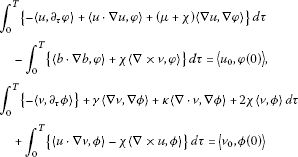
  and

  $${\int }_0^T\{-〈b,{\partial }_{\tau }\psi 〉+\nu 〈\mathrm{\nabla }b,\mathrm{\nabla }\psi 〉+〈u\cdot \mathrm{\nabla }b,\psi 〉-〈b\cdot \mathrm{\nabla }u,\psi 〉\}d\tau =〈b_0,\psi (0)〉.$$

• 3. The energy inequality, that is,

  

  (3.1)

Theorem 3.1 Let $u_0,b_0\in H_{\sigma }^1({\mathbb{R}}^3)$ with $v_0\in H^1({\mathbb{R}}^3)$. Assume that $(u,v,b)$ is a weak solution to (1.1), (1.2) on some interval $[0,T]$. If

$$\mathrm{\Phi }(T)\equiv {\int }_0^T{\parallel u_{x_3}\parallel }_{L^{\alpha }}^{\beta }dt<\mathrm{\infty },$$

(3.2)

where

$$\frac{3}{\alpha }+\frac{2}{\beta }\le 1,\alpha \ge 3,$$

then the solution $(u,v,b)$ can be extended smoothly beyond $t=T$.

4 Proof of Theorem 3.1

Proof Multiplying the first equation of (1.1) by u and integrating with respect to x on ${\mathbb{R}}^3$, using integration by parts, we obtain

$$\frac{1}{2}\frac{d}{dt}{\parallel u(t)\parallel }_{L^2}^2+(\mu +\chi ){\parallel \mathrm{\nabla }u(t)\parallel }_{L^2}^2={\int }_{{\mathbb{R}}^3}b\cdot \mathrm{\nabla }b\cdot udx+\chi {\int }_{{\mathbb{R}}^3}(\mathrm{\nabla }\times v)\cdot udx.$$

(4.1)

Similarly, we get

$$\frac{1}{2}\frac{d}{dt}{\parallel v(t)\parallel }_{L^2}^2+\gamma {\parallel \mathrm{\nabla }v(t)\parallel }_{L^2}^2+\kappa {\parallel \mathrm{\nabla }\cdot v\parallel }_{L^2}^2+2\chi {\parallel v\parallel }_{L^2}^2=\chi {\int }_{{\mathbb{R}}^3}(\mathrm{\nabla }\times u)\cdot vdx$$

(4.2)

and

$$\frac{1}{2}\frac{d}{dt}{\parallel b(t)\parallel }_{L^2}^2+\nu {\parallel \mathrm{\nabla }b(t)\parallel }_{L^2}^2={\int }_{{\mathbb{R}}^3}b\cdot \mathrm{\nabla }u\cdot bdx.$$

(4.3)

Summing up (4.1)-(4.3), we deduce that

(4.4)

By integration by parts and the Cauchy inequality, we obtain

$$\chi {\int }_{{\mathbb{R}}^3}(\mathrm{\nabla }\times v)\cdot udx+\chi {\int }_{{\mathbb{R}}^3}(\mathrm{\nabla }\times u)\cdot vdx\le \chi {\parallel \mathrm{\nabla }u\parallel }_{L^2}^2+\chi {\parallel v\parallel }_{L^2}^2.$$

(4.5)

Using integration by parts, we obtain

$${\int }_{{\mathbb{R}}^3}b\cdot \mathrm{\nabla }b\cdot udx+{\int }_{{\mathbb{R}}^3}b\cdot \mathrm{\nabla }u\cdot bdx=0.$$

(4.6)

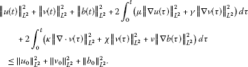
Combining (4.4)-(4.6) yields

Integrating with respect to t, we have

(4.7)

Differentiating (1.1) with respect to $x_3$, we obtain

$$\{\begin{array}{c}{\partial }_t{u}_{x_3}-(\mu +\chi )\mathrm{\Delta }{u}_{x_3}+u_{x_3}\cdot \mathrm{\nabla }u+u\cdot \mathrm{\nabla }{u}_{x_3}-b_{x_3}\cdot \mathrm{\nabla }b-b\cdot \mathrm{\nabla }{b}_{x_3}\hfill \\ +\mathrm{\nabla }{(p+\frac{1}{2}{|b|}^2)}_{x_3}-\chi \mathrm{\nabla }\times v_{x_3}=0,\hfill \\ {\partial }_t{v}_{x_3}-\gamma \mathrm{\Delta }{v}_{x_3}-\kappa \mathrm{\nabla }\cdot \mathrm{\nabla }{v}_{x_3}+2\chi v_{x_3}+u_{x_3}\cdot \mathrm{\nabla }v+u\cdot \mathrm{\nabla }{v}_{x_3}-\chi \mathrm{\nabla }\times u_{x_3}=0,\hfill \\ {\partial }_t{b}_{x_3}-\nu \mathrm{\Delta }{b}_{x_3}+u_{x_3}\cdot \mathrm{\nabla }b+u\cdot \mathrm{\nabla }{b}_{x_3}-b_{x_3}\cdot \mathrm{\nabla }u-b\cdot \mathrm{\nabla }{u}_{x_3}=0.\hfill \end{array}$$

(4.8)

Taking the inner product of $u_{x_3}$ with the first equation of (4.8) and using integration by parts yield

(4.9)

Similarly, we get

(4.10)

and

(4.11)

Combining (4.9)-(4.11) yields

(4.12)

Using integration by parts and the Cauchy inequality, we obtain

$$\chi {\int }_{{\mathbb{R}}^3}(\mathrm{\nabla }\times v_{x_3})\cdot u_{x_3}dx+\chi {\int }_{{\mathbb{R}}^3}(\mathrm{\nabla }\times u_{x_3})\cdot v_{x_3}dx\le \chi {\parallel \mathrm{\nabla }{u}_{x_3}\parallel }_{L^2}^2+\chi {\parallel v_{x_3}\parallel }_{L^2}^2.$$

(4.13)

Using integration by parts, we have

$${\int }_{{\mathbb{R}}^3}b\cdot \mathrm{\nabla }{b}_{x_3}\cdot u_{x_3}dx+{\int }_{{\mathbb{R}}^3}b\cdot \mathrm{\nabla }{u}_{x_3}\cdot b_{x_3}dx=0.$$

(4.14)

Combining (4.12)-(4.14) yields

(4.15)

In what follows, we estimate $I_j$ ($j=1,2,\dots ,5$). By integration by parts and the Hölder inequality, we obtain

$$I_1\le C{\parallel \mathrm{\nabla }{u}_{x_3}\parallel }_{L^2}{\parallel u_{x_3}\parallel }_{L^{\varrho }}{\parallel u\parallel }_{L^{3\alpha }},$$

where

$$\frac{1}{\varrho }+\frac{1}{3\alpha }=\frac{1}{2},2\le \varrho \le 6.$$

It follows from the interpolating inequality that

$${\parallel u_{x_3}\parallel }_{L^{\varrho }}\le C{\parallel u_{x_3}\parallel }_{L^2}^{1-3(\frac{1}{2}-\frac{1}{\varrho })}{\parallel \mathrm{\nabla }{u}_{x_3}\parallel }_{L^2}^{3(\frac{1}{2}-\frac{1}{\varrho })}.$$

From (2.2), we get

$$\begin{array}{rcl}{I}_1& \le & C{\parallel \mathrm{\nabla }{u}_{x_3}\parallel }_{L^2}{\parallel u_{x_3}\parallel }_{L^2}^{1-3(\frac{1}{2}-\frac{1}{\varrho })}{\parallel \mathrm{\nabla }{u}_{x_3}\parallel }_{L^2}^{3(\frac{1}{2}-\frac{1}{\varrho })}{\parallel \mathrm{\nabla }u\parallel }_{L^2}^{\frac{2}{3}}{\parallel u_{x_3}\parallel }_{L^{\alpha }}^{\frac{1}{3}}\\ \le & C{\parallel \mathrm{\nabla }{u}_{x_3}\parallel }_{L^2}^{1+3(\frac{1}{2}-\frac{1}{\varrho })}{\parallel u_{x_3}\parallel }_{L^2}^{1-3(\frac{1}{2}-\frac{1}{\varrho })}{\parallel \mathrm{\nabla }u\parallel }_{L^2}^{\frac{2}{3}}{\parallel u_{x_3}\parallel }_{L^{\alpha }}^{\frac{1}{3}}\\ \le & \frac{\mu }{2}{\parallel \mathrm{\nabla }{u}_{x_3}\parallel }_{L^2}^2+C{\parallel u_{x_3}\parallel }_{L^2}^2{\parallel \mathrm{\nabla }u\parallel }_{L^2}^{2q}{\parallel u_{x_3}\parallel }_{L^{\alpha }}^q,\end{array}$$

where

$$q=\frac{2}{3-9(\frac{1}{2}-\frac{1}{\varrho })}=\frac{2}{3(1-\frac{1}{\alpha })}.$$

When $\alpha \ge 3$, we have $2q\le 2$, and the application of the Young inequality yields

$$I_1\le \frac{\mu }{2}{\parallel \mathrm{\nabla }{u}_{x_3}\parallel }_{L^2}^2+C{\parallel u_{x_3}\parallel }_{L^2}^2({\parallel \mathrm{\nabla }u\parallel }_{L^2}^2+{\parallel u_{x_3}\parallel }_{L^{\alpha }}^{\delta }),$$

(4.16)

where

$$\frac{3}{\alpha }+\frac{2}{\delta }=1.$$

From integration by parts and the Hölder inequality, we obtain

$$\begin{array}{rcl}{I}_2& \le & C{\parallel \mathrm{\nabla }b\parallel }_{L^2}{\parallel b_{x_3}\parallel }_{L^{\frac{2\alpha }{\alpha -2}}}{\parallel u_{x_3}\parallel }_{L^{\alpha }}\le C{\parallel \mathrm{\nabla }b\parallel }_{L^2}{\parallel u_{x_3}\parallel }_{L^{\alpha }}{\parallel b_{x_3}\parallel }_{L^2}^{1-\frac{3}{\alpha }}{\parallel \mathrm{\nabla }{b}_{x_3}\parallel }_{L^2}^{\frac{3}{\alpha }}\\ \le & \frac{\nu }{6}{\parallel \mathrm{\nabla }{b}_{x_3}\parallel }_{L^2}^2+{\parallel \mathrm{\nabla }b\parallel }_{L^2}^{\frac{2\alpha }{2\alpha -3}}{\parallel u_{x_3}\parallel }_{L^{\alpha }}^{\frac{2\alpha }{2\alpha -3}}{\parallel b_{x_3}\parallel }_{L^2}^{\frac{2\alpha -6}{2\alpha -3}}\\ \le & \frac{\nu }{6}{\parallel \mathrm{\nabla }{b}_{x_3}\parallel }_{L^2}^2+C({\parallel \mathrm{\nabla }b\parallel }_{L^2}^2+{\parallel u_{x_3}\parallel }_{L^{\alpha }}^{\delta }){\parallel b_{x_3}\parallel }_{L^2}^{\frac{2\alpha -6}{2\alpha -3}},\end{array}$$

(4.17)

where

$$\frac{3}{\alpha }+\frac{2}{\delta }=1.$$

Similarly,

$$\begin{array}{rcl}{I}_3& \le & C{\parallel \mathrm{\nabla }v\parallel }_{L^2}{\parallel v_{x_3}\parallel }_{L^{\frac{2\alpha }{\alpha -2}}}{\parallel u_{x_3}\parallel }_{L^{\alpha }}\\ \le & C{\parallel \mathrm{\nabla }v\parallel }_{L^2}{\parallel u_{x_3}\parallel }_{L^{\alpha }}{\parallel v_{x_3}\parallel }_{L^2}^{1-\frac{3}{\alpha }}{\parallel \mathrm{\nabla }{v}_{x_3}\parallel }_{L^2}^{\frac{3}{\alpha }}\\ \le & \frac{\gamma }{2}{\parallel \mathrm{\nabla }{v}_{x_3}\parallel }_{L^2}^2+{\parallel \mathrm{\nabla }v\parallel }_{L^2}^{\frac{2\alpha }{2\alpha -3}}{\parallel u_{x_3}\parallel }_{L^{\alpha }}^{\frac{2\alpha }{2\alpha -3}}{\parallel v_{x_3}\parallel }_{L^2}^{\frac{2\alpha -6}{2\alpha -3}}\\ \le & \frac{\gamma }{2}{\parallel \mathrm{\nabla }{v}_{x_3}\parallel }_{L^2}^2+C({\parallel \mathrm{\nabla }v\parallel }_{L^2}^2+{\parallel u_{x_3}\parallel }_{L^{\alpha }}^{\delta }){\parallel v_{x_3}\parallel }_{L^2}^{\frac{2\alpha -6}{2\alpha -3}},\end{array}$$

(4.18)

and

$$\begin{array}{rcl}{I}_4& \le & C{\parallel \mathrm{\nabla }b\parallel }_{L^2}{\parallel b_{x_3}\parallel }_{L^{\frac{2\alpha }{\alpha -2}}}{\parallel u_{x_3}\parallel }_{L^{\alpha }}\\ \le & C{\parallel \mathrm{\nabla }b\parallel }_{L^2}{\parallel u_{x_3}\parallel }_{L^{\alpha }}{\parallel b_{x_3}\parallel }_{L^2}^{1-\frac{3}{\alpha }}{\parallel \mathrm{\nabla }{b}_{x_3}\parallel }_{L^2}^{\frac{3}{\alpha }}\\ \le & \frac{\nu }{6}{\parallel \mathrm{\nabla }{b}_{x_3}\parallel }_{L^2}^2+{\parallel \mathrm{\nabla }b\parallel }_{L^2}^{\frac{2\alpha }{2\alpha -3}}{\parallel u_{x_3}\parallel }_{L^{\alpha }}^{\frac{2\alpha }{2\alpha -3}}{\parallel b_{x_3}\parallel }_{L^2}^{\frac{2\alpha -6}{2\alpha -3}}\\ \le & \frac{\nu }{6}{\parallel \mathrm{\nabla }{b}_{x_3}\parallel }_{L^2}^2+C({\parallel \mathrm{\nabla }b\parallel }_{L^2}^2+{\parallel u_{x_3}\parallel }_{L^{\alpha }}^{\delta }){\parallel b_{x_3}\parallel }_{L^2}^{\frac{2\alpha -6}{2\alpha -3}},\end{array}$$

(4.19)

where

$$\frac{3}{\alpha }+\frac{2}{\delta }=1.$$

By integration by parts and the inequality, we have

$$\begin{array}{rcl}{I}_5& \le & C{\parallel \mathrm{\nabla }{b}_{x_3}\parallel }_{L^2}{\parallel b_{x_3}\parallel }_{L^{\sigma }}{\parallel u\parallel }_{L^{3\alpha }}\\ \le & C{\parallel \mathrm{\nabla }{b}_{x_3}\parallel }_{L^2}{\parallel b_{x_3}\parallel }_{L^2}^{1-3(\frac{1}{2}-\frac{1}{\sigma })}{\parallel \mathrm{\nabla }{b}_{x_3}\parallel }_{L^2}^{3(\frac{1}{2}-\frac{1}{\sigma })}{\parallel \mathrm{\nabla }u\parallel }_{L^2}^{\frac{2}{3}}{\parallel u_{x_3}\parallel }_{L^2}^{\frac{1}{3}}\\ \le & \frac{\nu }{6}{\parallel \mathrm{\nabla }{b}_{x_3}\parallel }_{L^2}^2+C{\parallel b_{x_3}\parallel }_{L^2}^2{\parallel \mathrm{\nabla }u\parallel }_{L^2}^{2q}{\parallel u_{x_3}\parallel }_{L^{\alpha }}^q,\end{array}$$

where

$$q=\frac{2}{3(1-\frac{1}{\alpha })}.$$

When $\alpha \ge 3$, we have $2q\le 2$, and the application of the Young inequality yields

$$I_5\le \frac{\nu }{6}{\parallel \mathrm{\nabla }{b}_{x_3}\parallel }_{L^2}^2+C{\parallel b_{x_3}\parallel }_{L^2}^2({\parallel \mathrm{\nabla }u\parallel }_{L^2}^2+{\parallel u_{x_3}\parallel }_{L^{\alpha }}^{\delta }),$$

(4.20)

where

$$\frac{3}{\alpha }+\frac{2}{\delta }=1.$$

Combining (4.15)-(4.20) yields

From the Gronwall inequality, we get

(4.21)

Multiplying the first equation of (1.1) by $-\mathrm{\Delta }u$ and integrating with respect to x on ${\mathbb{R}}^3$, and then using integration by parts, we obtain

(4.22)

Similarly, we get

(4.23)

and

(4.24)

Collecting (4.22)-(4.24) yields

(4.25)

Thanks to integration by parts and the Cauchy inequality, we get

$$-\chi {\int }_{{\mathbb{R}}^3}(\mathrm{\nabla }\times v)\cdot \mathrm{\Delta }udx-\chi {\int }_{{\mathbb{R}}^3}(\mathrm{\nabla }\times u)\cdot \mathrm{\Delta }vdx\le \chi {\parallel \mathrm{\Delta }u\parallel }_{L^2}^2+\chi {\parallel \mathrm{\nabla }v\parallel }_{L^2}^2.$$

(4.26)

It follows from (4.25)-(4.26) and integration by parts that

(4.27)

In what follows, we estimate $J_i$ ($i=1,\dots ,5$).

By (2.3) and the Young inequality, we deduce that

$$\begin{array}{rcl}{J}_1& \le & C{\parallel \mathrm{\nabla }u\parallel }_{L^3}^3\le C{\parallel \mathrm{\nabla }u\parallel }_{L^2}^{\frac{3}{2}}{\parallel {\mathrm{\nabla }}_{\tilde{x}}\mathrm{\nabla }u\parallel }_{L^2}{\parallel \mathrm{\nabla }{u}_{x_3}\parallel }_{L^2}^{\frac{1}{2}}\\ \le & \frac{\mu }{10}{\parallel {\mathrm{\nabla }}_{\tilde{x}}\mathrm{\nabla }u\parallel }_{L^2}^2+C{\parallel \mathrm{\nabla }u\parallel }_{L^2}^3{\parallel \mathrm{\nabla }{u}_{x_3}\parallel }_{L^2}\\ \le & \frac{\mu }{10}{\parallel {\mathrm{\nabla }}_{\tilde{x}}\mathrm{\nabla }u\parallel }_{L^2}^2+C({\parallel \mathrm{\nabla }u\parallel }_{L^2}^2+{\parallel \mathrm{\nabla }{u}_{x_3}\parallel }_{L^2}^2){\parallel \mathrm{\nabla }u\parallel }_{L^2}^2.\end{array}$$

(4.28)

By (2.3) and the Young inequality, we have

$$\begin{array}{rcl}{J}_2& \le & {\parallel \mathrm{\nabla }u\parallel }_{L^3}{\parallel \mathrm{\nabla }b\parallel }_{L^3}^2\\ \le & C{\parallel \mathrm{\nabla }u\parallel }_{L^2}^{\frac{1}{2}}{\parallel {\mathrm{\nabla }}_{\tilde{x}}\mathrm{\nabla }u\parallel }_{L^2}^{\frac{1}{3}}{\parallel \mathrm{\nabla }{u}_{x_3}\parallel }_{L^2}^{\frac{1}{6}}{\parallel \mathrm{\nabla }b\parallel }_{L^2}{\parallel {\mathrm{\nabla }}_{\tilde{x}}\mathrm{\nabla }b\parallel }_{L^2}^{\frac{2}{3}}{\parallel \mathrm{\nabla }{b}_{x_3}\parallel }_{L^2}^{\frac{1}{3}}\\ \le & \frac{\mu }{10}{\parallel {\mathrm{\nabla }}_{\tilde{x}}\mathrm{\nabla }u\parallel }_{L^2}^2+C{\parallel \mathrm{\nabla }u\parallel }_{L^2}^{\frac{3}{5}}{\parallel \mathrm{\nabla }{u}_{x_3}\parallel }_{L^2}^{\frac{1}{5}}{\parallel \mathrm{\nabla }b\parallel }_{L^2}^{\frac{6}{5}}{\parallel {\mathrm{\nabla }}_{\tilde{x}}\mathrm{\nabla }b\parallel }_{L^2}^{\frac{4}{5}}{\parallel \mathrm{\nabla }{b}_{x_3}\parallel }_{L^2}^{\frac{2}{5}}\\ \le & \frac{\mu }{10}{\parallel {\mathrm{\nabla }}_{\tilde{x}}\mathrm{\nabla }u\parallel }_{L^2}^2+\frac{\nu }{6}{\parallel {\mathrm{\nabla }}_{\tilde{x}}\mathrm{\nabla }b\parallel }_{L^2}^2+C{\parallel \mathrm{\nabla }u\parallel }_{L^2}{\parallel \mathrm{\nabla }{u}_{x_3}\parallel }_{L^2}^{\frac{1}{3}}{\parallel \mathrm{\nabla }b\parallel }_{L^2}^2{\parallel \mathrm{\nabla }{b}_{x_3}\parallel }_{L^2}^{\frac{2}{3}}\\ \le & \frac{\mu }{10}{\parallel {\mathrm{\nabla }}_{\tilde{x}}\mathrm{\nabla }u\parallel }_{L^2}^2+\frac{\nu }{6}{\parallel {\mathrm{\nabla }}_{\tilde{x}}\mathrm{\nabla }b\parallel }_{L^2}^2\\ +C{\parallel \mathrm{\nabla }b\parallel }_{L^2}^2({\parallel \mathrm{\nabla }u\parallel }_{L^2}^2+{\parallel \mathrm{\nabla }{u}_{x_3}\parallel }_{L^2}^2+{\parallel \mathrm{\nabla }{b}_{x_3}\parallel }_{L^2}^2).\end{array}$$

(4.29)

Similarly, we obtain

(4.30)

(4.31)

and

$$\begin{array}{rcl}{J}_5& \le & {\parallel \mathrm{\nabla }u\parallel }_{L^3}{\parallel \mathrm{\nabla }b\parallel }_{L^3}^2\\ \le & \frac{\mu }{10}{\parallel {\mathrm{\nabla }}_{\tilde{x}}\mathrm{\nabla }u\parallel }_{L^2}^2+\frac{\nu }{6}{\parallel {\mathrm{\nabla }}_{\tilde{x}}\mathrm{\nabla }b\parallel }_{L^2}^2\\ +C{\parallel \mathrm{\nabla }b\parallel }_{L^2}^2({\parallel \mathrm{\nabla }u\parallel }_{L^2}^2+{\parallel \mathrm{\nabla }{u}_{x_3}\parallel }_{L^2}^2+{\parallel \mathrm{\nabla }{b}_{x_3}\parallel }_{L^2}^2).\end{array}$$

(4.32)

Combining (4.27)-(4.32) yields

(4.33)

From (4.33), the Gronwall inequality, (4.7) and (4.21), we know that $(u,v,b)\in L^{\mathrm{\infty }}(0,T;H^1({\mathbb{R}}^3))$. Thus, $(u,v,b)$ can be extended smoothly beyond $t=T$. We have completed the proof of Theorem 3.1. □

Author’s contributions

The author completed the paper herself. The author read and approved the final manuscript.

References

Gala S: Regularity criteria for the 3D magneto-micropolar fluid equations in the Morrey-Campanato space. Nonlinear Differ. Equ. Appl. 2010, 17: 181-194. 10.1007/s00030-009-0047-4
Ortega-Torres EE, Rojas-Medar MA: On the uniqueness and regularity of the weak solution for magneto-micropolar fluid equations. Rev. Mat. Apl. 1996, 17: 75-90.
Ortega-Torres EE, Rojas-Medar MA: On the regularity for solutions of the micropolar fluid equations. Rend. Semin. Mat. Univ. Padova 2009, 122: 27-37.
Ortega-Torres EE, Rojas-Medar MA: Magneto-micropolar fluid motion: global existence of strong solutions. Abstr. Appl. Anal. 1999, 4: 109-125. 10.1155/S1085337599000287
Rojas-Medar MA: Magneto-micropolar fluid motion: existence and uniqueness of strong solutions. Math. Nachr. 1997, 188: 301-319. 10.1002/mana.19971880116
Rojas-Medar MA, Boldrini JL: Magneto-micropolar fluid motion: existence of weak solutions. Rev. Mat. Complut. 1998, 11: 443-460.
Yuan B: Regularity of weak solutions to magneto-micropolar fluid equations. Acta Math. Sci. 2010, 30: 1469-1480.
Yuan J: Existence theorem and blow-up criterion of the strong solutions to the magneto-micropolar fluid equations. Math. Methods Appl. Sci. 2008, 31: 1113-1130. 10.1002/mma.967
Zhang Z, Yao A, Wang X: A regularity criterion for the 3D magneto-micropolar fluid equations in Triebel-Lizorkin spaces. Nonlinear Anal. 2011, 74: 2220-2225. 10.1016/j.na.2010.11.026
Wang Y, Hu L, Wang Y: A Beale-Kato-Madja criterion for magneto-micropolar fluid equations with partial viscosity. Bound. Value Probl. 2011., 2011: Article ID 128614
Eringen AC: Theory of micropolar fluids. J. Math. Mech. 1966, 16: 1-18.
Lukaszewicz G Modeling and Simulation in Science, Engineering and Technology. In Micropolar Fluids: Theory and Applications. Birkhäuser, Boston; 1999.
Galdi GP, Rionero S: A note on the existence and uniqueness of solutions of the micropolar fluid equations. Int. J. Eng. Sci. 1977, 15: 105-108. 10.1016/0020-7225(77)90025-8
Yamaguchi N: Existence of global strong solution to the micropolar fluid system in a bounded domain. Math. Methods Appl. Sci. 2005, 28: 1507-1526. 10.1002/mma.617
Dong B, Chen Z: Regularity criteria of weak solutions to the three-dimensional micropolar flows. J. Math. Phys. 2009., 50: Article ID 103525
Wang Y, Chen Z: Regularity criterion for weak solution to the 3D micropolar fluid equations. J. Appl. Math. 2011., 2011: Article ID 456547
Dong B, Jia Y, Chen Z: Pressure regularity criteria of the three-dimensional micropolar fluid flows. Math. Methods Appl. Sci. 2011, 34: 595-606. 10.1002/mma.1383
Wang Y, Yuan H: A logarithmically improved blow-up criterion for smooth solutions to the 3D micropolar fluid equations. Nonlinear Anal., Real World Appl. 2012, 13: 1904-1912. 10.1016/j.nonrwa.2011.12.018
Lifschitz AE: Magnetohydrodynamics and spectral theory. 4. In Developments in Electromagnetic Theory and Applications. Kluwer Academic, Dordrecht; 1989.
Sermange M, Temam R: Some mathematical questions related to the MHD equations. Commun. Pure Appl. Math. 1983, 36: 635-666. 10.1002/cpa.3160360506
Cao C, Wu J: Two regularity criteria for the 3D equations. J. Differ. Equ. 2010, 248: 2263-2274. 10.1016/j.jde.2009.09.020
Gala S: Extension criterion on regularity for weak solutions to the 3D MHD equations. Math. Methods Appl. Sci. 2010, 33: 1496-1503.
He C, Xin Z: On the regularity of solutions to the magnetohydrodynamic equations. J. Differ. Equ. 2005, 213: 235-254. 10.1016/j.jde.2004.07.002
He C, Wang Y: On the regularity for weak solutions to the magnetohydrodynamic equations. J. Differ. Equ. 2007, 238: 1-17. 10.1016/j.jde.2007.03.023
He C, Wang Y: Remark on the regularity for weak solutions to the magnetohydrodynamic equations. Math. Methods Appl. Sci. 2008, 31: 1667-1684. 10.1002/mma.992
Lei Z, Zhou Y: BKM criterion and global weak solutions for magnetohydrodynamics with zero viscosity. Discrete Contin. Dyn. Syst., Ser. A 2009, 25: 575-583.
Wang Y, Zhao H, Wang Y: A logarithmally improved blow up criterion of smooth solutions for the three-dimensional MHD equations. Int. J. Math. 2012., 23: Article ID 1250027
Wu J: Viscous and inviscid magneto-hydrodynamics equations. J. Anal. Math. (Jerus.) 1997, 73: 251-265. 10.1007/BF02788146
Zhou Y: Remarks on regularities for the 3D MHD equations. Discrete Contin. Dyn. Syst. 2005, 12: 881-886.
Zhou Y, Gala S: Regularity criteria for the solutions to the 3D MHD equations in the multiplier space. Z. Angew. Math. Phys. 2010, 61: 193-199. 10.1007/s00033-009-0023-1
Zhou Y, Gala S: A new regularity criterion for weak solutions to the viscous MHD equations in terms of the vorticity field. Nonlinear Anal. 2010, 72: 3643-3648. 10.1016/j.na.2009.12.045
Admas RA: Sobolev Spaces. Academic Press, New York; 1975.
Galdi GP: An Introduction to the Mathematical Theory of the Navier-Stokes Equations. Springer, New York; 1994. Vols I, II
Ladyzhenskaya OA: Mathematical Theory of Viscous Incompressible Flow. 2nd edition. Gordon & Breach, New York; 1969. English translation
Author information
Authors and Affiliations
Corresponding author
Additional information
Competing interests
The author declares that she has no competing interests.
Rights and permissions
Open Access This article is distributed under the terms of the Creative Commons Attribution 2.0 International License (https://creativecommons.org/licenses/by/2.0), which permits unrestricted use, distribution, and reproduction in any medium, provided the original work is properly cited.
About this article
Cite this article
Wang, Y. Regularity criterion for a weak solution to the three-dimensional magneto-micropolar fluid equations. Bound Value Probl 2013, 58 (2013). https://doi.org/10.1186/1687-2770-2013-58
Received:
Accepted:
Published:
DOI: https://doi.org/10.1186/1687-2770-2013-58