
Abstract
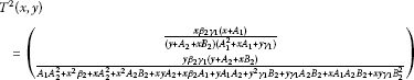
We investigate the global asymptotic behavior of solutions of the following anti-competitive system of rational difference equations:
where the parameters , , , and are positive numbers and the initial conditions are arbitrary nonnegative numbers. We find the basins of attraction of all attractors of this system, which are the equilibrium points and period-two solutions.
MSC:39A10, 39A11.
1 Introduction
A first-order system of difference equations
where , are continuous functions is competitive if is non-decreasing in x and non-increasing in y, and is non-increasing in x and non-decreasing in y.
System (1) where the functions f and g have a monotonic character opposite of the monotonic character in competitive system will be called anti-competitive.
We consider the following anti-competitive system of difference equations:
where the parameters , , , and are positive numbers and the initial conditions are arbitrary nonnegative numbers. In the classification of all linear fractional systems in [1], System (2) was mentioned as System (16, 39).
Competitive and cooperative systems of the form (1) were studied by many authors such as Clark and Kulenović [2], Clark, Kulenović and Selgrade [3], Hirsch and Smith [4], Kulenović and Ladas [5], Kulenović and Merino [6], Kulenović and Nurkanović [7, 8], Garić-Demirović, Kulenović and Nurkanović [9, 10], Smith [11, 12] and others.
The study of anti-competitive systems started in [13] and has advanced since then (see [14, 15]). The principal tool of the study of anti-competitive systems is the fact that the second iterate of the map associated with an anti-competitive system is a competitive map, and so the elaborate theory for such maps developed recently in [4, 16, 17] can be applied.
The main result on the global behavior of System (2) is the following theorem.
Theorem 1 (a) If , then is a unique equilibrium, and the basin of attraction of this equilibrium is (see Figure 1(a)).

Basins of attraction
(b) If and , then there exist two equilibrium points: which is a repeller and which is an interior saddle point, and minimal period-two solutions and which are locally asymptotically stable. There exists a set such that , and is an invariant subset of the basin of attraction of . The set is a graph of a strictly increasing continuous function of the first variable on an interval and separates into two connected and invariant components, namely
which satisfy (see Figure 1(b)):
(i) If , then
and
(ii) If , then
and
(c) If , then (see Figure 1(c))
(i) There exist two equilibrium points: which is a repeller and which is a non-hyperbolic, and an infinite number of minimal period-two solutions

for , that belong to the segment of the line (15) in the first quadrant.
(ii) All minimal period-two solutions and the equilibrium are stable but not asymptotically stable.
(iii) There exists a family of strictly increasing curves , , for and
that emanate from and , for all , such that the curves are pairwise disjoint, the union of all the curves equals . Solutions with initial points in converge to and solutions with an initial point in have even-indexed terms converging to and odd-indexed terms converging to ; solutions with an initial point in have even-indexed terms converging to and odd-indexed terms converging to .
(d) If , then System (2) has two equilibrium points: which is a repeller and which is locally asymptotically stable, and minimal period-two solutions and which are saddle points. The basin of attraction of the equilibrium point is the set
and solutions with an initial point in have even-indexed terms converging to and odd-indexed terms converging to , solutions with an initial point in have even-indexed terms converging to and odd-indexed terms converging to (see Figure 1(d)).
2 Preliminaries
We now give some basic notions about systems and maps in the plane of the form (1).
Consider a map on a set , and let . The point is called a fixed point if . An isolated fixed point is a fixed point that has a neighborhood with no other fixed points in it. A fixed point is an attractor if there exists a neighborhood of E such that as for ; the basin of attraction is the set of all such that as . A fixed point E is a global attractor on a set if E is an attractor and is a subset of the basin of attraction of E. If T is differentiable at a fixed point E, and if the Jacobian has one eigenvalue with modulus less than one and a second eigenvalue with modulus greater than one, E is said to be a saddle. See [18] for additional definitions.
Here we give some basic facts about the monotone maps in the plane, see [11, 16, 17, 19]. Now, we write System (2) in the form
where the map T is given as
The map T may be viewed as a monotone map if we define a partial order on so that the positive cone in this new partial order is the fourth quadrant. Specifically, for , we say that if and . Two points are said to be related if or . Also, a strict inequality between points may be defined as if and . A stronger inequality may be defined as if and . A map is strongly monotone if implies that for all . Clearly, being related is an invariant under iteration of a strongly monotone map. Differentiable strongly monotone maps have Jacobian with constant sign configuration
The mean value theorem and the convexity of may be used to show that T is monotone, as in [20].
For , define for to be the usual four quadrants based at x and numbered in a counterclockwise direction, for example, .
The following definition is from [11].
Definition 1 Let be a nonempty subset of . A competitive map is said to satisfy condition (O+) if for every x, y in , implies , and T is said to satisfy condition (O−) if for every x, y in , implies .
The following theorem was proved by de Mottoni-Schiaffino for the Poincaré map of a periodic competitive Lotka-Volterra system of differential equations. Smith generalized the proof to competitive and cooperative maps [11].
Theorem 2 Let be a nonempty subset of . If T is a competitive map for which (O+) holds then for all , is eventually componentwise monotone. If the orbit of x has compact closure, then it converges to a fixed point of T. If instead (O−) holds, then for all , is eventually componentwise monotone. If the orbit of x has compact closure in , then its omega limit set is either a period-two orbit or a fixed point.
The following result is from [11], with the domain of the map specialized to be the Cartesian product of intervals of real numbers. It gives a sufficient condition for conditions (O+) and (O−).
Theorem 3 Let be the Cartesian product of two intervals in . Let be a competitive map. If T is injective and for all then T satisfies (O+). If T is injective and for all then T satisfies (O−).
Next two results are from [17, 21].
Theorem 4 Let T be a competitive map on a rectangular region . Let be a fixed point of T such that is nonempty (i.e., is not the NW or SE vertex of ), and T is strongly competitive on Δ. Suppose that the following statements are true.
-
a.
The map T has a extension to a neighborhood of .
-
b.
The Jacobian matrix of T at has real eigenvalues λ, μ such that , where , and the eigenspace associated with λ is not a coordinate axis.
Then there exists a curve through that is invariant and a subset of the basin of attraction of , such that is tangential to the eigenspace at , and is the graph of a strictly increasing continuous function of the first coordinate on an interval. Any endpoints of in the interior of are either fixed points or minimal period-two points. In the latter case, the set of endpoints of is a minimal period-two orbit of T.
Theorem 5 (Kulenović & Merino)
Let , be intervals in with endpoints , and , with endpoints respectively, with and , where and . Let T be a competitive map on a rectangle and . Suppose that the following hypotheses are satisfied:
-
1.
and T is strongly competitive on .
-
2.
The point is the only fixed point of T in .
-
3.
The map T is continuously differentiable in a neighborhood of .
-
4.
At least one of the following statements is true:
-
a.
T has no minimal period two orbits in .
-
b.
and only for .
-
5.
is a saddle point.
Then the following statements are true.
-
(i)
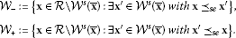
The stable manifold is connected and it is the graph of a continuous increasing curve with endpoints in . is divided by the closure of into two invariant connected regions (“below the stable set”), and (“above the stable set”), where
-
(ii)
The unstable manifold is connected, and it is the graph of a continuous decreasing curve.
-
(iii)
For every , eventually enters the interior of the invariant set , and for every , eventually enters the interior of the invariant set .
-
(iv)
Let and be the endpoints of , where . For every and every such that , there exists such that , and for every and every such that , there exists such that .

3 Linearized stability analysis
Lemma 1
-
(i)
If , then System (2) has a unique equilibrium point .
-
(ii)
If , then System (2) has two equilibrium points and , , .
Proof The equilibrium point of System (2) satisfies the following system of equations:
It is easy to see that is one equilibrium point for all values of the parameters, and is a positive equilibrium point if . Indeed, substituting from the first equation in (4) in the second equation in (4), we obtain that satisfies the following equation:
By using Descartes’ theorem, we have that equation (5) has one positive equilibrium if the condition
is satisfied, i.e., . □
Theorem 6
-
(i)
If , then is locally asymptotically stable.
-
(ii)
If , then is non-hyperbolic.
-
(iii)
If , then is a repeller.
Proof The map T associated to System (2) is of the form (3). The Jacobian matrix of T at the equilibrium is
and
The corresponding characteristic equation has the following form:
from which .
-
(i)
If , then , i.e., is locally asymptotically stable.
-
(ii)
If , then , which implies that is non-hyperbolic.
-
(iii)
If , then , which implies that is a repeller.
□
Theorem 7
-
(1)
Assume that and
(8)
Then the positive equilibrium is a saddle point.
-
(2)
Assume that
(9)
Then the positive equilibrium is a non-hyperbolic point and
-
(3)
Assume that
(10)
Then the positive equilibrium is locally asymptotically stable.
Proof The Jacobian matrix of T at the equilibrium is of the form (7) and the corresponding characteristic equation has the following form:
where

Hence, for , we have , , so . Since
we obtain
Similarly,
where
Now, for the positive equilibrium, it holds

If , then for all , which implies that is a saddle point. If , then for (, ).
Now we have three cases: , or . Functions and are increasing for .
-
(1)
If , then , i.e., and . So,

from which it follows
i.e.,
Now we have
so we can see that the conditions (8) and (6) are sufficient for to be a saddle point.
-
(2)
If , then , hence , i.e.,
from which
If conditions (12) and (6) are satisfied, then
holds, i.e., is a non-hyperbolic point of the form
-
(3)
If , then and
from which
Hence, if conditions (13) and (6) are satisfied, then
holds, so is a locally asymptotically stable. □
4 Periodic character of solutions
In this section, we give the existence and local stability of period-two solutions.
Lemma 2 Assume that . Then System (2) has the following minimal period-two solutions:
If
then System (2) has an infinite number of minimal period-two solutions of the form

for , located along the line
Proof The second iterate of T is (25). Equilibrium curves of the map are
and
We get period-two solutions as the intersection point of equilibrium curves (16) and (17) in the first quadrant. If , , then System (16), (17) is reduced to the equation
and the positive solution of this equation is
If , , then System (16), (17) is reduced to the equation
with the positive solution
On the other hand, if , , then we have
that is
and

Therefore, it must be in order to get any positive solution. By eliminating the term from (18) and using condition (9), we get
which implies
hence
Now, by eliminating y and the term from (19), we get the identity
If , we have
So, periodic solutions are located along line (15) with endpoints given by (14) using conditions (9). It is easy to see that if . □
Let , then the corresponding Jacobian matrix of the map has the following form:
where , , , .
Lemma 3 Assume that . Then the following statements are true.
-
(a)
The points are non-hyperbolic fixed points for the map , and both of them have eigenvalues and .
-
(b)
Eigenvectors corresponding to the eigenvalues and are not parallel to coordinate axes.
Proof (a) From (15) we have . Since
by implicit differentiation of equations and at the point , we obtain
Since , , and , from (22), we get
The characteristic polynomial of the matrix (21) at the point is of the form
Now, using (22) we have , and since
we get , and due to Vieta’s formulas and condition (23), it follows
i.e., .
(b) Eigenvectors corresponding to the eigenvalues and are and . By condition (23) it is easy to see that these vectors are not parallel to the coordinate axes. □
Lemma 4 The periodic points and given by (14) are
-
(a)
locally asymptotically stable if and ,
-
(b)
non-hyperbolic if ,
-
(c)
saddle points if .
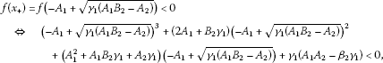
Proof We have that
and characteristic eigenvalues are
Now,

Therefore,

On the other hand, we have
and the corresponding eigenvalues are
so it comes to the same conclusion! □
5 Global results
In this section, we present the results on the global dynamics of System (2).
Lemma 5 Every solution of System (2) satisfies
-
1.
, , .
-
2.
If , then , .
The map T satisfies:
-
3.
, where , that is, is an invariant box.
-
4.
is an attracting box, that is .
Proof From System (2), we have

for , and
for . Furthermore, we get
i.e.,
so it follows that , if .
Proof of 3. and 4. is an immediate checking. □
Lemma 6 The map is injective and , for all and .
Proof (i) Here we prove that map T is injective, which implies that is injective. Indeed, implies that
By solving System (24) with respect to , or , , we obtain that .
-
(ii)
The map is of the form
 (25)
(25)

and
where

Now, we obtain
where

and the Jacobian matrix of is invertible for all and . □
Corollary 1 The competitive map satisfies the condition (O+). Consequently, the sequences , , , of every solution of System (2) are eventually monotone.
Proof It immediately follows from Lemma 6, Theorem 2 and 3. □
Lemma 7 Assume . System (2) has period-two solutions (14) and
-
(a)
If , , then
and
-
(b)
If , , then
and
Proof (a) For all , , we have

and by induction,

Now, we have

and

□
Lemma 8 The map associated to System (2) satisfies the following:
Proof Since is injective, then . □
Proof of Theorem 1 Case 1
Equilibrium is unique (see Lemma 1), and by Lemma 5, every solution of System (2) belongs to
which is an invariant box. In view of Corollary 1 and Theorem 2, every solution converges to minimal period-two solutions or . System (2) has no minimal period-two solutions (Lemma 2). So, every solution of System (2) converges to .
Case 2 and
By Lemmas 1, 2, 4 and Theorems 6 and 7, there exist two equilibrium points: which is a repeller and which is a saddle point, and minimal period-two solutions and which are locally asymptotically stable. Clearly is strongly competitive and it is easy to check that the points and are locally asymptotically stable for as well. System (2) can be decomposed into the system of the even-indexed and odd-indexed terms as follows:
The existence of the set with the stated properties follows from Lemmas 6, 2, 7, 8, Corollary 1, Theorems 4 and 5.
Case 3
Cases (i) and (ii) from (c) in Theorem 1 are the consequence of Lemmas 1, 2, 4 and Theorems 6 and 7.
Since is strongly competitive and points and , for all , are non-hyperbolic points of the map , by Lemmas 1, 6, 2, 3, 7, Corollary 1, Theorems 2, 5, 6 and 7, it follows that all conditions of Theorem 4 are satisfied for the map with . By Lemma 7, it is clear that
Case 4
Lemma 2 implies that System (2) has minimal period-two solutions (14). Furthermore, Corollary 1 and Theorem 2 imply that all solutions of System (2) converge to an equilibrium or minimal period-two solutions, and since, by Theorem 6, is a repeller, all solutions converge to (which is, in view of Theorem 7, locally asymptotically stable) or minimal period-two solutions (14). The points and are saddle points of the strongly competitive map ; and by Lemma 7, the stable manifold of (under ) is
and the stable manifold of (under ) is
and each of these stable manifolds is unique. This implies that the basin of attraction of the equilibrium point is the set
and Lemma 7 completes the conclusion (d) of Theorem 1. □
References
Camouzis E, Kulenović MRS, Ladas G, Merino O: Rational systems in the plane - open problems and conjectures. J. Differ. Equ. Appl. 2009, 15: 303–323. 10.1080/10236190802125264
Clark D, Kulenović MRS: On a coupled system of rational difference equations. Comput. Math. Appl. 2002, 43: 849–867. 10.1016/S0898-1221(01)00326-1
Clark CA, Kulenović MRS, Selgrade JF: On a system of rational difference equations. J. Differ. Equ. Appl. 2005, 11: 565–580. 10.1080/10236190412331334464
Hirsch M, Smith H: Monotone Dynamical Systems. Ordinary Differential Equations 2. In Handbook of Differential Equations. Elsevier, Amsterdam; 2005:239–357.
Kulenović MRS, Ladas G: Dynamics of Second Order Rational Difference Equations with Open Problems and Conjectures. Chapman and Hall/CRC, Boca Raton; 2001.
Kulenović MRS, Merino O: Discrete Dynamical Systems and Difference Equations with Mathematica. Chapman and Hall/CRC, Boca Raton; 2002.
Kulenović MRS, Nurkanović M: Asymptotic behavior of a system of linear fractional difference equations. J. Inequal. Appl. 2005, 2005: 127–144.
Kulenović MRS, Nurkanović M: Asymptotic behavior of a competitive system of linear fractional difference equations. Adv. Differ. Equ. 2006, 2006: 1–13.
Brett A, Garić-Demirović M, Kulenović MRS, Nurkanović M: Global behavior of two competitive rational systems of difference equations in the plane. Commun. Appl. Nonlinear Anal. 2009, 16: 1–18.
Garic-Demirović M, Kulenović MRS, Nurkanović M: Global behavior of four competitive rational systems of difference equations in the plane. Discrete Dyn. Nat. Soc. 2009., 2009: Article ID 153058
Smith HL: Planar competitive and cooperative difference equations. J. Differ. Equ. Appl. 1998, 3: 335–357. 10.1080/10236199708808108
Smith HL: The discrete dynamics of monotonically decomposable maps. J. Math. Biol. 2006, 53: 747–758. 10.1007/s00285-006-0004-3
Kalabušić S, Kulenović MRS: Dynamics of certain anti-competitive systems of rational difference equations in the plane. J. Differ. Equ. Appl. 2011, 17: 1599–1615. 10.1080/10236191003730506
Garic-Demirović M, Nurkanović M: Dynamics of an anti-competitive two dimensional rational system of difference equations. Sarajevo J. Math. 2011, 7(19):39–56.
Kalabušić, S, Kulenović, MRS, Pilav, E: Global dynamics of anti-competitive systems in the plane (submitted)
Kulenović MRS, Merino O: Competitive-exclusion versus competitive-coexistence for systems in the plane. Discrete Contin. Dyn. Syst., Ser. B 2006, 6: 1141–1156.
Kulenović MRS, Merino O: Global bifurcation for discrete competitive systems in the plane. Discrete Contin. Dyn. Syst., Ser. B 2009, 12: 133–149.
Robinson C: Stability, Symbolic Dynamics, and Chaos. CRC Press, Boca Raton; 1995.
Kulenović MRS, Merino O: Invariant manifolds for competitive discrete systems in the plane. Int. J. Bifurc. Chaos 2010, 20: 2471–2486. 10.1142/S0218127410027118
Clark D, Kulenović MRS, Selgrade JF: Global asymptotic behavior of a two dimensional difference equation modelling competition. Nonlinear Anal. TMA 2003, 52: 1765–1776. 10.1016/S0362-546X(02)00294-8
Kulenović MRS, Merino O: A global attractivity result for maps with invariant boxes. Discrete Contin. Dyn. Syst., Ser. B 2006, 6: 97–110.
Acknowledgements
The authors are very grateful to Professor M.R.S. Kulenović for his valuable suggestions. They thank also the referees for their useful comments.
Author information
Authors and Affiliations
Corresponding author
Additional information
Competing interests
The authors declare that they have no competing interests.
Authors’ contributions
Both authors contributed to each part of this study equally and read and approved the final version of the manuscript.
Authors’ original submitted files for images
Below are the links to the authors’ original submitted files for images.
Rights and permissions
Open Access This article is distributed under the terms of the Creative Commons Attribution 2.0 International License (https://creativecommons.org/licenses/by/2.0), which permits unrestricted use, distribution, and reproduction in any medium, provided the original work is properly cited.
About this article
Cite this article
Moranjkić, S., Nurkanović, Z. Basins of attraction of certain rational anti-competitive system of difference equations in the plane. Adv Differ Equ 2012, 153 (2012). https://doi.org/10.1186/1687-1847-2012-153
Received:
Accepted:
Published:
DOI: https://doi.org/10.1186/1687-1847-2012-153