
Abstract
A discrete semi-ratio-dependent predator-prey system with Holling type IV functional response and time delay is investigated. It is proved the general nonautonomous system is permanent and globally attractive under some appropriate conditions. Furthermore, if the system is periodic one, some sufficient conditions are established, which guarantee the existence and global attractivity of positive periodic solutions. We show that the conditions for the permanence of the system and the global attractivity of positive periodic solutions depend on the delay, so, we call it profitless.
Introduction
Recently, many authors have explored the dynamics of a class of the nonautonomous semi-ratio-dependent predator-prey systems with functional responses

where x 1(t), x 2(t) stand for the population density of the prey and the predator at time t, respectively. In (1.1), it has been assumed that the prey grows logistically with growth rate r 1 (t) and carrying capacity r 1(t)/a 11(t) in the absence of predation. The predator consumes the prey according to the functional response f (t, x 1(t)) and grows logistically with growth rate r 2 (t) and carrying capacity x 1(t)/a 21(t) proportional to the population size of the prey (or prey abundance). a 21 (t) is a measure of the food quality that the prey provides, which is converted to predator birth. For more background and biological adjustments of system (1.1), we can see [1–7] and the references cited therein.
In 1965, Holling [8] proposed three types of functional response functions according to different kinds of species on the foundation of experiments. Recently, many authors have explored the dynamics of predator-prey systems with Holling type functional responses [1, 3, 4, 7, 9–14]. Furthermore, some authors [15, 16] have also described a type IV functional response that is humped and that declines at high prey densities. This decline may occur due to prey group defense or prey toxicity. Ding et al. [5] proposed the following semi-ratio-dependent predator-prey system with nonmonotonic functional response and time delay

Using Gaines and Mawhins continuation theorem of coincidence degree theory and by constructing an appropriate Lyapunov functional, they obtained a set of sufficient conditions which guarantee the existence and global attractivity of positive periodic solutions of the system (1.2).
Already, many authors [13, 14, 17–23] have argued that the discrete time models governed by difference equations are more appropriate than the continuous ones when the populations have non-overlapping generations. Based on the above discussion, in this article, we consider the following discrete semi-ratio-dependent predator-prey system with Holling type IV functional response and time delay

where x 1(k), x 2(k) stand for the density of the prey and the predator at k th generation, respectively. m ≠ 0 is a constant. τ denotes the time delay due to negative feedback of the prey population.
For convenience, throughout this article, we let Z, Z +, R +, and R 2 denote the sets of all integers, nonnegative integers, nonnegative real numbers, and two-dimensional Euclidian vector space, respectively, and use the notations: f u = sup k∈Z+{f(k)}, f l = inf k∈Z+{f(k)}, for any bounded sequence {f(k)}.
In this article, we always assume that for all i, j = 1, 2, (H
1) r
i
(k), a
ij
(k) are all positive bounded sequences such that  ,
,  ; τ is a nonnegative integer.
By a solution of system (1.3), we mean a sequence {x 1(k), x 2(k)} which defines for Z + and which satisfies system (1.3) for Z +. Motivated by application of system (1.3) in population dynamics, we assume that solutions of system (1.3) satisfy the following initial conditions

The exponential forms of system (1.3) assure that the solution of system (1.3) with initial conditions (1.4) remains positive.
The principle aim of this article is to study the dynamic behaviors of system (1.3), such as permanence, global attractivity, existence, and global attractivity of positive periodic solutions. To the best of our knowledge, no work has been done for the discrete non-autonomous difference system (1.3). The organization of this article is as follows. In the next section, we explore the permanent property of the system (1.3). We study globally attractive property of the system (1.3) and the periodic property of system (1.3). At last, the conclusion ends with brief remarks.
Permanence
First, we introduce a definition and some lemmas which are useful in the proof of the main results of this section.
Definition 2.1. System (1.3) is said to be permanent, if there are positive constants m i and M i , such that for each positive solution (x 1(k), x 2(k)) T of system (1.3) satisfies

Lemmas 2.1 and 2.2 are Theorem 2.1 in [19] and Lemma 2.2 in [14].
Lemma 2.1. Let
 . For any fixed k, g(k, r) is a non-decreasing function, and for k ≥ k
0, the following inequalities hold:
. For any fixed k, g(k, r) is a non-decreasing function, and for k ≥ k
0, the following inequalities hold:

If y(k 0) ≤ u(k 0), then y(k) ≤ u(k) for all k ≥ k 0.
Now let us consider the following discrete single species model:

where {a(k)} and {b(k)} are strictly positive sequences of real numbers defined for k ∈ Z + and 0 < a l ≤ a u , 0 < b l ≤ b u .
Lemma 2.2. Any solution of system (2.1) with initial condition N(0) > 0
satisfies

where

Set

Theorem 2.1. Assume that (H 1) holds, assume further that
(H
2) 
holds. Then system (1.3) is permanent.
Proof. Let x(k) = (x 1(k), x 2(k)) T be any positive solution of system (1.3) with initial conditions (1.4), from the first equation of the system (1.3), it follows that

and

It follows from (2.2) that

which implies that

which, together with (2.3), produces,

By applying Lemmas 2.1 and 2.2 to (2.6), we have

For any ε > 0 small enough, it follows from (2.7) that there exists enough large K 1 such that for k ≥ K 1,

Substituting (2.8) into the second equation of system (1.3), it follows that

By applying Lemmas 2.1 and 2.2 to (2.9), we obtain

Setting ε → 0 in above inequality, we have

Condition (H 2) implies that we could choose ε > 0 small enough such that

From (2.7) and (2.10) that there exists enough large K 2 > K 1 such that for i = 1, 2
and k ≥ K 2,

Thus, for k > K 2 + τ, by (2.13) and the first equation of system (1.3), we have

where

And

It follows from (2.14) that

which implies that

this combined with (2.16)

By applying Lemmas 2.1 and 2.2 to (2.19), it follows that

where

Setting ε → 0 in above inequality, we have

where

and

From (2.22) we know that there exists enough large K 3 > K 2 such that for k ≥ K 3,

(2.25) combining with the second equation of the system (1.3) leads to,

By applying Lemmas 2.1 and 2.2 to (2.26), we have

Setting ε → 0 in above inequality, one has

Consequently, combining (2.7), (2.11), (2.22) with (2.28), system (1.3) is permanent. This completes the proof of Theorem 2.1.
Global attractivity
Now, we study the global attractivity of the positive solution of system (1.3). To do so, we first introduce a definition and prove a lemma which will be useful to our main result.
Definition 3.1. A positive solution (x
1(k), x
2(k)) T of system (1.3) is said to be globally attractive if each other solution  of system (1.3) satisfies

Lemma 3.1. For any two positive solutions (x
1(k), x
2(k)) T
and
of system (1.3), we have

where

Proof. It follows from the first equation of system (1.3) that

where

Hence,

Since

and

By the mean value theorem, one has

Thus we can easily obtain (3.1) by substituting (3.3) and (3.4) into (3.2). The proof of Lemma 3.1 is completed.
Now we are in the position of stating the main result on the global attractivity of system (1.3).
Theorem 3.1. In addition to (H 1)-(H 2), assume further that (H 3) there exist positive constants λ 1, λ 2 such that

holds, where ρ, ϱ, σ are defined by (3.23). Then for any two positive solutions (x
1(k), x
2(k)) T
and
of system (1.3), one has

Proof. Let (x
1(k), x
2(k)) T and be two arbitrary solutions of system (1.3). To prove Theorem 3.1, for the first equation of system (1.3), we will consider the following three steps,
Step 1. We let

It follows from (3.1) that

where

By the mean value theorem, we have

that is,

where ξ
1(k) lies between x
1(k) and  . So, we have

According to Theorem 2.1, there exists a positive integer k
0 such that m
i
≤ x
i
(k)  for k > k
0 and i = 1, 2. Therefore, for all k > k
0 + τ, we can obtain that
for k > k
0 and i = 1, 2. Therefore, for all k > k
0 + τ, we can obtain that

Step 2. Let

Then

Step 3. Let

By a simple calculation, it follows that

We now define

Then for all k > k 0 + τ, it follows from (3.10)-(3.14) that

We let

It follows from the second equation of system (1.3) that

that is,

It follows from (3.17) that

Similar to the argument of (3.7)-(3.9), we can obtain

Therefore,

We now define a Lyapunov function as:

It is easy to see that V (k) > 0 and V (k 0 +τ) < +∞. Calculating the difference of V along the solution of system (1.3), we have that for k ≥ k 0 + τ,

where

Summing both sides of (3.22) from k 0 + τ to k, it derives that

it then follows from (3.24) that for k > k 0 + τ,

that is,

Then

Therefore, we can easily obtain that

This completes the proof of Theorem 3.1.
In the following section, we consider the periodic property of system (1.3).
Existence and global attractivity of positive periodic solutions
In this section, we assume that all the coefficients of system (1.3) are positive sequences with common periodic ω, where ω is a fixed positive integer, stands for the prescribed common period of the parameters in system (1.3), then the system (1.3) is an ω-periodic system for this case. And so the coefficients of system (1.3) will naturally satisfy assumption (H 1).
In order to obtain the existence of positive periodic solutions of system (1.3), we first make the following preparations that will be basic for this section.
Let X, Z be two Banach spaces. Consider an operator equation

where L : DomL ∩ X → Z is a linear operator and λ, is a parameter. Let P and Q denote two projectors such that

Denote that J : ImQ → KerL is an isomorphism of ImQ onto KerL. Recall that a linear mapping L : DomL ∩ X → Z with KerL = L -1(0) and ImL = L(DomL), will be called a Fredholm mapping if the following two conditions hold:
-
(i)
KerL has a finite dimension;
-
(ii)
ImL is closed and has a finite codimension.
Recall also that the codimension of ImL is dimension of Z/ ImL, i.e., the dimension of the cokernel coker L of L.
When L is a Fredholm mapping, its index is the integer IndL = dim KerL - codim ImL.
We shall say that a mapping N is L-compact on Ω if the mapping  is continuous,
  is bounded and
  is compact. i.e., it is continuous and
  is relatively compact, where K
P
: ImL → DomL ∩ KerP is an inverse of the restriction L
P
of L to DomL ∩ KerP, so that LK
P
= I and K
P
= I - P. The following Lemma is from Gains and Mawhin [24].
is relatively compact, where K
P
: ImL → DomL ∩ KerP is an inverse of the restriction L
P
of L to DomL ∩ KerP, so that LK
P
= I and K
P
= I - P. The following Lemma is from Gains and Mawhin [24].
Lemma 4.1. (Continuation Theorem) Let X, Z be two Banach spaces and L be a Fredholm mapping of index zero. Assume that
 is L-compact on
 with Ω open bounded in X. Furthermore assume:
-
(a)
For each λ ∈ (0, 1), x ∈ ∂Ω ∩ DomL, Lx ≠ λNx,
-
(b)
QNx ≠ 0 for each × ∈ ∂Ω ∩ KerL,
-
(c)
deg{JQNx, Ω ∩ KerL, 0} ≠ 0.
Then the equation Lx = Nx has at least one solution lying in Dom
 .
.
For convenience in the following discussion, we will use the notation below:

where {f(k)} is an ω-periodic sequence.
Lemma 4.2. Let f : Z → R be ω-periodic, i.e., f(k + ω) = f(k), then for any fixed k 1, k 2 ∈ I ω and any k ∈ Z, one has

Denote

for a = (a 1, a 2) T ∈ R 2, define |a| = max{a 1, a 2}. Let l ω ⊂ l 2 denote the subspace of all ω-periodic sequences equipped with the usual supremum norm ||·||, i.e.,

Then it follows that l ω is a finite dimensional Banach space.
Let

Then it follows that
 and
and
 are both closed linear subspaces of l
ω
and
are both closed linear subspaces of l
ω
and

Set

Theorem 4.1. Assume that
(H
4) 
holds. Then periodic system (1.3) has at least one positive ω-periodic solution. Proof. Since solutions of system (1.3) remained positive for k ≥ 0, we let

then system (1.3) is reformulated as:

It is easy to see that if (4.2) has one ω-periodic solution  , then (1.3) has one positive ω-periodic solution
  . Therefore, to complete the proof, it is only to show that (4.2) has at least one ω-periodic solution.
To use Lemma 4.1, we take X = Z = l ω . Denote by L : X → X the difference operator given by Lu = {(Lu)(k)} with (Lu)(k) = u(k + 1) - u(k), for u ∈ X and k ∈ Z, and N : X → X as follows:

for any u ∈ X, and k ∈ Z. It is trivial to see that L is a bounded linear operator and

then it follows that L is a Fredholm mapping of index zero.
Define

It is not difficult to show that P and Q are continuous projectors such that

hence, by a simple computation, we can find that the generalized inverse (to L) K P : ImL → DomL ∩ KerP exists and is given by

Thus QN : X → Z and K P (I - Q)N : X → X are given by

and

Consider the operator equation Lu = λNu, λ ∈ (0, 1), we have

Assume that u ∈ X is a solution of (4.3) for a certain λ ∈ (0, 1). Summing on both sides of (4.3) from 0 to ω - 1 with respect to k, we obtain

From (4.3) and (4.4), we have

Noting that u = {(u 1(k), u 2(k)) T } ∈ X. Then there exist ξ i , η i ∈ I ω , i = 1, 2 such that

From (4.4) and (4.6), we obtain

that is,

which, together with (4.5) and Lemma 4.2, leads to,

On the other hand, by (4.4), (4.6), and (4.8), we also have

which yields

The above inequality, together with (4.5) and Lemma 4.2, leads to,

From (4.4) and (4: 5), we can deduce

that is,

and along with (4.5) and Lemma 4.2, we have

Thus we derive from (4.8) and (4.14) that

On the other hand, by (4.4), (4.6), and (4.8), we get

which implies

The above inequality, together with (4.5) and Lemma 4.2, leads to,

It follows from (4.11) and (4.18) that

Clearly, H i (i = 1, 2) are independent of λ.
Next, for μ ∈ 0[1], we consider the following algebraic equations:

where (u 1(k), u 2(k)) T ∈ R 2. By the similar argument of (4.7), (4.10), (4.13), and (4.17), we can derive the solutions (u 1(k), u 2(k)) T of (4.20) that satisfy

Denote H = H 1 + H 2 + C, here, C is taken sufficiently large such that C ≥ |K 1| + |k 1| + |K 2| + |k 2|. Now we take Ω = {(u 1(k), u 2(k)) T ∈ X : || (u 1(k), u 2(k)) T ||< H}. Now we check the conditions of Lemma 4.1.
-
(a)
From (4.15) and (4.19), one can see that for each λ ∈ (0, 1), u ∈ ∂Ω ∩ DomL, Lu ≠ λNu.
-
(b)
When (u 1(k), u 2(k)) T ∈ ∂Ω ∩ KerL = ∂Ω ∩ R 2, (u 1(k), u 2(k)) T is a constant vector in R 2 with || (u 1, u 2) T || = H. If

then (u 1(k), u 2(k)) T is the constant solution of system (4.20) with μ = 1. From (4.21), we have || (u 1, u 2) T ||< H. This contradiction implies that for each u ∈ ∂Ω ∩ KerL, QNu ≠ 0.
-
(c)
we will prove that condition (c) of Lemma 4.1 is satisfied. To this end, we define ϕ : DomL × 0[1] → X by
 (4.22)

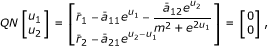
where μ ∈ 0[1] is a parameter. When (u 1, u 2) T ∈ ∂Ω ∩ KerL, (u 1, u 2) T is a constant vector in R 2 with || (u 1, u 2) T || = H. From (4.21), we know that ϕ(u 1, u 2, μ) ≠ (0, 0) T on ∂Ω ∩ KerL. Hence, due to homotopy invariance theorem of topology degree and taking J = I : ImQ → KerL, we have

It is not difficult to see that the following algebraic equation:

has a unique solution  . Thus

Finally, we will prove that N is L- compact on . For any  , we have

Hence, is bounded. Obviously,  is continuous.
And also

For any , k
1, k
2 ∈ I
ω
, without loss of generality, let k
2
> k
1, then we have

Thus, the set  is equicontinuous and uniformly bounded.
By applying Ascoli-Arzela theorem, one can see that  is compact. Consequently, N is L-compact.
By now we have verified all the requirements of Lemma 4.1. Hence system (4.2) has at least one ω-periodic solution. This ends the proof of Theorem 4.1.
By constructing similar Lyapunov function to those of Theorem 3.1, and using Theorem 4.1, we have the following Theorem 4.2.
Theorem 4.2. Assume that the conditions of (H 2)-(H 4) hold. Then the positive periodic solution of periodic system (1.3) is globally attractive.
Concluding remarks
In this article, a discrete time semi-ratio-dependent predator-prey system with Holling type IV functional response and time delay is investigated. By using comparison theorem and further developing the analytical technique of [14, 21], we prove the system (1.3) is permanent under some appropriate conditions. Further, by constructing the suitable Lyapunov function, we show that the system (1.3) is globally attractive under some appropriate conditions. If the system (1.3) is periodic one, by using the continuous theorem of coincidence degree theory and Theorem 3.1, some sufficient conditions are established, which guarantee the existence and global attractivity of positive periodic solutions of the system (1.3). We note that the time delay has an effect on the permanence and the global attractivity of periodic solution of system (1.3), but time delay has no effect on the existence of positive periodic solutions.
References
Leslie PH: Some further notes on the use of matrices in population mathematics. Biometrika 1948, 35: 213-245.
Leslie PH, Gower JC: A properties of a stochastic model for the predator-prey type of interaction between two species. Biometrika 1960,47(3-4):219-234. 10.1093/biomet/47.3-4.219
Aziz-Alaoui MA, Daher Okiye M: Boundeness and global stability for a predator-prey model with modified Leslie-Gower and Holling-type II schemes. Appl. Math. Lett 2003,16(7):1069-1075. 10.1016/S0893-9659(03)90096-6
Nindjina AF, Aziz-Alaoui MA, Cadivel M: Analysis of a predator-prey model with modified Leslie-Gower and Holling-type II schemes with time delay. Non-linear Anal. Real World Appl 2006,7(5):1104-1118. 10.1016/j.nonrwa.2005.10.003
Ding XH, Lu C, Liu MZ: Periodic solutions for a semi-ratio-dependent predator-prey system with nonmonotonic functional response and time delay. Nonlinear Anal. Real World Appl 2008,9(3):762-775. 10.1016/j.nonrwa.2006.12.008
Ivlev VS: Experimental Ecology of the Feeding of Fishes. New Haven: Yale University Press; 1961.
Tanner JT: The stability and the intrinsic growth rates of prey and predator populations. Ecology 1975, 56: 855-867. 10.2307/1936296
Holling CS: The functional response of predator to prey density and its role in mimicry and population regulation. Mem. Entomol. Soc. Can 1965, 45: 1-60.
Meng XZ, Xu WJ, Chen LS: Profitless delays for a nonautonomous Lotka-Volterra predator-prey almost periodic system with dispersion. Appl. Math. Comput 2007,188(1):365-378. 10.1016/j.amc.2006.09.133
Meng XZ, Chen LS: Almost periodic solution of non-autonomous Lotka-Volterra predator-prey dispersal system with delays. J. Theor. Biol 2006,243(4):562-574. 10.1016/j.jtbi.2006.07.010
Xu R, Chaplain MAJ: Persistence and global stability in a delayed predator-prey system with Michaelis-Menten type functional response. Appl. Math. Comput 2002,130(2-3):441-455. 10.1016/S0096-3003(01)00111-4
Xu R, Chaplain MAJ, Davidson FA: Periodic solutions for a predator-prey model with Holling-type functional response and time delays. Appl. Math. Comput 2005,161(2):637-654. 10.1016/j.amc.2003.12.054
Yang XT: Uniform persistence and periodic solutions for a discrete predator-prey system with delays. J. Math. Anal. Appl 2006,316(1):161-177. 10.1016/j.jmaa.2005.04.036
Chen FD: Permanence of a discrete n-species food-chain system with time delays. Appl. Math. Comput 2007,185(1):719-726. 10.1016/j.amc.2006.07.079
Freedman HI: Deterministic Mathematical Models in Population Ecology. New York: Marcel Dekker; 1980.
Sokol W, Howell JA: Kinetics of phenol oxidation by washed cells. Biotechnol. Bioeng 1980, 23: 2039-2049.
Agarwal RP, Wong PJY: Advance Topics in Difference Equations. Dordrecht: Kluwer Publisher; 1997.
Chen FD, Wu LP, Li Z: Permanence and global attractivity of the discrete Gilpin-Ayala type population model. Comput. Math. Appl 2007,53(8):1214-1227. 10.1016/j.camwa.2006.12.015
Wang L, Wang MQ: Ordinary Difference Equation. Xinjiang University Press, Xinjiang; 1991.
Wu LP, Chen FD, Li Z: Permanence and global attractivity of a discrete Schoener's competition model with delays. Math. Comput. Model 2009,49(7-8):1607-1617. 10.1016/j.mcm.2008.06.004
Chen FD: Permanence of a discrete N-species cooperation system with time delays and feedback controls. Appl. Math. Comput 2007,186(1):23-29. 10.1016/j.amc.2006.07.084
Liu ZJ, Chen LS: Positive periodic solution of a general discrete non-autonomous difference system of plankton allelopathy with delays. J. Comput. Appl. Math 2006,197(2):446-456. 10.1016/j.cam.2005.09.023
Lu HY: Permanence of a discrete nonlinear prey-competition system with delays. Discr. Dyn. Nat. Soc 2009, 15. Article ID 605254
Gaines RE, Mawhin JL: Coincidence Degree and Nonlinear Differential Equations. Volume 568. Lecture Notes in Mathematics, Springer, Berlin; 1977.
Acknowledgements
The authors are grateful to the Associate Editor, R. L. Pouso, and referees for a number of helpful suggestions that have greatly improved our original submission. This work is supported by the National Natural Science Foundation of China (No.70901016), Excellent Talents Program of Liaoning Educational Committee (No.2008RC15), and Innovation Method Fund of China (No.2009IM010400-1-39).
Author information
Authors and Affiliations
Corresponding authors
Additional information
Competing interests
The authors declare that they have no competing interests.
Authors' contributions
HL carried out the main part of this article, WW corrected the main theorems. All authors read and approved the final manuscript.
Rights and permissions
Open Access This article is distributed under the terms of the Creative Commons Attribution 2.0 International License (https://creativecommons.org/licenses/by/2.0), which permits unrestricted use, distribution, and reproduction in any medium, provided the original work is properly cited.
About this article
Cite this article
Lu, H., Wang, W. Dynamics of a delayed discrete semi-ratio-dependent predator-prey system with Holling type IV functional response. Adv Differ Equ 2011, 7 (2011). https://doi.org/10.1186/1687-1847-2011-7
Received:
Accepted:
Published:
DOI: https://doi.org/10.1186/1687-1847-2011-7