
Abstract
In this paper, we will discuss asymptotic limit of non-isentropic compressible Euler-Maxwell system arising from plasma physics. Formally, we give some different limit systems according to the corresponding different scalings. Furthermore, some recent results about the convergence of non-isentropic compressible Euler-Maxwell system to the compressible Euler-Poisson equations will be given via the non-relativistic regime.
1 Introduction and the formal limits
Let n, u, and θ denote the scaled macroscopic density, mean velocity vector, and temperature of the electrons and E and B the scaled electric field and magnetic field, respectively. They are functions of a three-dimensional position vector  and of the time t > 0, where
  is the torus. The fields E and B are coupled to the particles through the Maxwell equations and act on the particles via the Lorentz force E + γu × B. These variables satisfy the scaled non-isentropic Euler-Maxwell system for plasma physics in a uniform background of non-moving ions with fixed density b(x) (see [1–3]):


In the system, Equations 1.1-1.3 are the mass, momentum, and energy balance laws, respectively, while (1.4)-(1.5) are the Maxwell equations. It is well known that two equations in (1.5) are redundant with two equations in (1.4) as soon as they are satisfied by the initial conditions. The non-dimensionalized parameters γ and ε can be chosen independently on each other, according to the desired scaling. Physically, γ and ε are proportional to  and the Debye length, where c is the speed of light. Thus, the limit γ → 0 is called the non-relativistic limit while the limit ε → 0 is called the quasi-neutral limit. Starting from one fluid and non-isentropic Euler-Maxwell system, we can derive some different limit systems according to the corresponding different scalings.
Case 1: Non-relativistic limit, Quasi-neutral limit
In this case, we first perform non-relativistic limit and then quasi-neutral limit.
Step 1: Let ε be fixed and γ → 0. Formally, we get the following system:


This limit is the Euler-Poisson system of compressible electron fluid.
Remark 1.1. Equations 1.10 implies B = 0 when the mean value of B(x, t) vanishes, i.e. m (B) = 0. Here,

denotes the mean value of a given scalar or vector function v(x, t) in
 with respect to x. Furthermore, equation ∇ × E = 0 in (1.11) with m(E) = 0 implies the existence of a potential function ϕ
0
such that
with respect to x. Furthermore, equation ∇ × E = 0 in (1.11) with m(E) = 0 implies the existence of a potential function ϕ
0
such that

Step 2: Set ε = 0 in Euler-Poisson system (1.7)-(1.11), we can obtain n - b(x) = 0, which is so-called quasi-neutrality in plasma physics. Then, (u, θ, ϕ) satisfy the following equations:


Remark 1.2. If the ion density b(x) is a constant, say b(x) = 1 for simplicity; then from (1.12)-(1.14), we see that (u, θ, ϕ) satisfy the non-isentropic incompressible Euler equations of ideal fluid:


Hence, one derives the non-isentropic incompressible Euler equations.
Case 2: Quasineutral limit, Non-relativistic limit
In this case, we take b(x) = 1 for simplicity. Contrarily to Case 1, we first perform quasineutral limit and then non-relativistic limit.
Step 1: Let γ be fixed and ε turns to zero, one can gets n - 1 = 0 (quasineutrality), and then we get from the Euler-Maxwell system (1.1)-(1.5) that


This is so-called the non-isentropic e-MHD equations.
Step 2: We set γ = 0 and get that

and the non-isentropic incompressible Euler equations 1.16-1.18 of ideal fluid from the e-MHD system (1.18)-(1.21).
Case 3: Combined quasineutral and non-relativistic limits
Similarly to Case 2, we still take b(x) = 1 for simplicity. Choose ε = γ and let ε = γ → 0, first it is easy to get from the Maxwell system (1.4)-(1.5) that n = 1 (quasi-neutrality) and

Then one gets the non-isentropic incompressible Euler equations 1.15-1.17 of ideal fluid from the Euler-Maxwell system (1.1)-(1.5).
The above formal limits are obvious, but it is very difficult to rigorously prove them, even in isentropic case, see [4–6]. Since usually it is required to deal with some complex related problems such as the oscillatory behavior of the electric fields, the initial layer problem, the sheath boundary layer problem, and the classical shock problem. The proofs of these convergence are based on the asymptotic expansion of multiple-scale and the careful energy methods, iteration scheme, the entropy methods, etc. In the following section, we will provide a rigorous convergence result when ε is fixed (especially we take ε = 1) and γ → 0. We state our result in the following section. For detail, see [7]. For the other results, see [4–6] and references therein.
2 Rigorous convergence
Let (n γ , u γ , θ γ , E γ , B γ ) be the classical solutions to problem (1.1)-(1.6) and assume that the initial conditions have the following asymptotic expansion with respect to γ:

Plugging the following ansatz:

into system (1.1)-(1.6), we obtain:
-
(1)
The leading profiles (n 0, u 0, θ 0, E 0, B 0) satisfy the following equations:
 (2.2)
(2.2) (2.3)
(2.3) (2.4)
(2.4) (2.5)
(2.5) (2.6)
(2.6) (2.7)
(2.7)


From (2.6), we may take B
0 = 0, and equation ∇ × E
0 = 0 in (2.5) implies the existence of a potential function ϕ
0 such that E
0 = -∇ϕ
0. Then Equations 2.2-2.5 become a non-isentropic compressible Euler-Poisson system and determine a unique smooth solution (n
0, u
0, ϕ
0) in the class m(ϕ
0) = 0 well defined on  with T
*
> 0. Here, we need the following compatibility conditions on (E
0, B
0):
with T
*
> 0. Here, we need the following compatibility conditions on (E
0, B
0):

where ϕ 0 satisfies

-
(2)
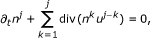
For any j ≥ 1, the profiles (n j , u j , θ j , E j , B j ) can be obtained by induction. Now, we assume that (n k , u k , θ k , E k , B k )0≤k≤j-1are smooth and already determined in previous steps. Then (n j , u j , θ j , E j , B j ) satisfy the following linearized equations:
 (2.10)
 (2.11)
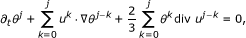 (2.12)
 (2.13)
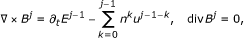 (2.14)
 (2.15)


where f
0 = 0,  and f
j-1((n
k , θ
k)
k≤j-1) is defined by
and f
j-1((n
k , θ
k)
k≤j-1) is defined by

Equations 2.14 are of curl-div type and they determine a unique smooth B
j in the class m(B
j ) = 0 in . Moreover, from div B
j = 0, we deduce the existence of a given vector function ω
j such that B
j = - ∇ × ω
j . Then, the first equation in (2.13) becomes ∇ × (E
j-∂
t
ωj-1) = 0. It follows that there is a potential function ϕ
j such that E
j = ∂
t
ωj-1- ∇ϕ
j with ω
0 = 0.
Then, (n j , u j , θ j , ϕ j ) solve a compressible linearized Euler-Poisson system:


where g j-1= f j-1+∂ t ω j-1. Then system (2.16)-(2.20) determines a unique smooth solution (n j, u j, θ j, ϕ j) j≥1in the class m(ϕ j) = 0, in the time interval [0, T *]. Since E j= ∂ t ω j-1- ∇ϕ j, we need the following compatibility conditions on (E j , B j ):

where ϕ j is determined by

for and m(ϕ
j ) = 0.
Proposition 2.1. Assume that the initial data (n
j
, u
j
, E
j
, B
j
)
j<0
are sufficiently smooth with n
0 > 0 in
 and satisfy the compatibility conditions (2.8)-(2.9) and (2.21)-(2.22). Then there exists a unique asymptotic expansion up to any order of the form (2.1), i.e. there exist the unique smooth profiles (n
j
u
j, E
j , B
j )
j<0, solutions of the problems (2.2)-(2.7) and (2.10)-(2.15) in the time interval [0, T
*]. In particular, the formal non-relativistic limit γ → 0 of the non-isentropic compressible Euler-Maxwell system (1.1)-(1.6) is the non-isentropic compressible Euler-Poisson system.
and satisfy the compatibility conditions (2.8)-(2.9) and (2.21)-(2.22). Then there exists a unique asymptotic expansion up to any order of the form (2.1), i.e. there exist the unique smooth profiles (n
j
u
j, E
j , B
j )
j<0, solutions of the problems (2.2)-(2.7) and (2.10)-(2.15) in the time interval [0, T
*]. In particular, the formal non-relativistic limit γ → 0 of the non-isentropic compressible Euler-Maxwell system (1.1)-(1.6) is the non-isentropic compressible Euler-Poisson system.
Set

where (n j , u j , θ j , E j , B j ) are those constructed in the previous Proposition 1.1.
For the convergence of the compressible Euler-Maxwell system (1.1)-(1.6), our main result is stated as follows.
Theorem 2.1. For any fixed integer
 and m ≥ 1, assume that the mean values of E
γ(x, t), B
γ(x, t) vanish and the ion density b(x) the initial data (n
j
, u
j
, θ
j
)
j≥0, satisfy the following conditions:
and m ≥ 1, assume that the mean values of E
γ(x, t), B
γ(x, t) vanish and the ion density b(x) the initial data (n
j
, u
j
, θ
j
)
j≥0, satisfy the following conditions:
-
 ,
, -
n 0, θ 0 ≥ δ > 0 for some constant δ,
-
m(b(x) - n 0) = m(n j ) = 0, j ≥ 1
 ,
,with N = m and s = m + s 0 + 3 hold. Furthermore, if

satisfy the compatibility condition

and initial condition

then, there exists T * ∈ (0, T *] such that problem (1.1)-(1.6) has a unique solution

Furthermore,

where (n j , u j , θ j , E j , B j )0≤j≤m are solutions to problems and C > 0 is a constant independent of γ.
References
Chen F: Introduction to Plasma Physics and Controlled Fusion. Volume 1. Plenum Press, New York; 1984.
Jerome JW: The Cauchy problem for compressible hydrodynamic-Maxwell systems: a local theory for smooth solutions. Diff Integral Equ 2003, 16: 1345–1368.
Dinklage A, Klinger T, Marx G, Schweikhard L: Plasma Physics. Lecture Notes in Physics. Volume 670. Springer, Berlin; 2005.
Peng YJ, Wang S: Convergence of compressible Euler-Maxwell equations to compressible Euler-Poisson equations. Chin Ann Math 2007,28(B):583–602.
Peng YJ, Wang S: Convergence of compressible Euler-Maxwell equations to incompressible Eule equations. J Comm PDE 2008, 33: 349–476. 10.1080/03605300701318989
Yang JW, Wang S: The non-relativistic limit of Euler-Maxwell equations for two-fluid plasma. Nonlinear Anal Theory Methods Appl 2010, 72: 1829–1840. 10.1016/j.na.2009.09.024
Yang JW, Wang S: Convergence of the nonisentropic Euler-Maxwell equations to compressible Euler-Poisson equations. J Math Phys 2009, 50: 123508. 10.1063/1.3267863
Acknowledgements
The authors cordially acknowledge partial support from the Research Initiation Project for High-level Talents (no. 201035) of North China University of Water Resources and Electric Power.
Author information
Authors and Affiliations
Corresponding author
Additional information
Competing interests
The authors declare that they have no competing interests.
Authors' contributions
All authors contributed equally to the manuscript and read and approved the final draft.
Rights and permissions
Open Access This article is distributed under the terms of the Creative Commons Attribution 2.0 International License (https://creativecommons.org/licenses/by/2.0), which permits unrestricted use, distribution, and reproduction in any medium, provided the original work is properly cited.
About this article
Cite this article
Yang, J., Gao, Q. & Zhang, Q. Scaling limits of non-isentropic Euler-Maxwell equations for plasmas. Adv Differ Equ 2011, 22 (2011). https://doi.org/10.1186/1687-1847-2011-22
Received:
Accepted:
Published:
DOI: https://doi.org/10.1186/1687-1847-2011-22