
Abstract
Background
Similarity of sequences is a key mathematical notion for Classification and Phylogenetic studies in Biology. It is currently primarily handled using alignments. However, the alignment methods seem inadequate for post-genomic studies since they do not scale well with data set size and they seem to be confined only to genomic and proteomic sequences. Therefore, alignment-free similarity measures are actively pursued. Among those, USM (Universal Similarity Metric) has gained prominence. It is based on the deep theory of Kolmogorov Complexity and universality is its most novel striking feature. Since it can only be approximated via data compression, USM is a methodology rather than a formula quantifying the similarity of two strings. Three approximations of USM are available, namely UCD (Universal Compression Dissimilarity), NCD (Normalized Compression Dissimilarity) and CD (Compression Dissimilarity). Their applicability and robustness is tested on various data sets yielding a first massive quantitative estimate that the USM methodology and its approximations are of value. Despite the rich theory developed around USM, its experimental assessment has limitations: only a few data compressors have been tested in conjunction with USM and mostly at a qualitative level, no comparison among UCD, NCD and CD is available and no comparison of USM with existing methods, both based on alignments and not, seems to be available.
Results
We experimentally test the USM methodology by using 25 compressors, all three of its known approximations and six data sets of relevance to Molecular Biology. This offers the first systematic and quantitative experimental assessment of this methodology, that naturally complements the many theoretical and the preliminary experimental results available. Moreover, we compare the USM methodology both with methods based on alignments and not. We may group our experiments into two sets. The first one, performed via ROC (Receiver Operating Curve) analysis, aims at assessing the intrinsic ability of the methodology to discriminate and classify biological sequences and structures. A second set of experiments aims at assessing how well two commonly available classification algorithms, UPGMA (Unweighted Pair Group Method with Arithmetic Mean) and NJ (Neighbor Joining), can use the methodology to perform their task, their performance being evaluated against gold standards and with the use of well known statistical indexes, i.e., the F-measure and the partition distance. Based on the experiments, several conclusions can be drawn and, from them, novel valuable guidelines for the use of USM on biological data. The main ones are reported next.
Conclusion
UCD and NCD are indistinguishable, i.e., they yield nearly the same values of the statistical indexes we have used, accross experiments and data sets, while CD is almost always worse than both. UPGMA seems to yield better classification results with respect to NJ, i.e., better values of the statistical indexes (10% difference or above), on a substantial fraction of experiments, compressors and USM approximation choices. The compression program PPMd, based on PPM (Prediction by Partial Matching), for generic data and Gencompress for DNA, are the best performers among the compression algorithms we have used, although the difference in performance, as measured by statistical indexes, between them and the other algorithms depends critically on the data set and may not be as large as expected. PPMd used with UCD or NCD and UPGMA, on sequence data is very close, although worse, in performance with the alignment methods (less than 2% difference on the F-measure). Yet, it scales well with data set size and it can work on data other than sequences. In summary, our quantitative analysis naturally complements the rich theory behind USM and supports the conclusion that the methodology is worth using because of its robustness, flexibility, scalability, and competitiveness with existing techniques. In particular, the methodology applies to all biological data in textual format. The software and data sets are available under the GNU GPL at the supplementary material web page.
Background
The notion of distance and similarity between two strings is a very important and widely studied one [1–4] since it plays a fundamental role in biological sequence analysis, phylogeny and classification. Classically, those notions hinge on sequence alignment methods. However, distance and similarity functions based on alignment methods do not scale well with data set size and they are no longer perceived as adequate now that entire genomes are available [5]. Moreover, they are not flexible, since they can only be used with genomic and proteomic sequences. Therefore, novel alignment-free functions are actively pursued, the ones based on textual compression being natural candidates because of the deep connection of compression with classification and modeling [6].
In this scenario, Li et al. [7] have devised a universal similarity metric for strings-a remarkable achievement since universality means it is a lower bound for all the computable distance and similarity functions, including all the ones so far considered for biological applications, e.g., [2–5]. Unfortunately, being the measure based on Kolmogorov complexity [8], it is not computable. However, one can still get a practical tool from such a beautiful theoretical finding since the Kolmogorov complexity of a string can be approximated via data compression [8]. This leaves open the problem of how to best approximate the universal measure, which can be regarded more as a methodology than a formula quantifying how similar two objects are. Three distinct functions have been proposed as an approximation to USM: UCD, NCD and CD. We point out that two of them have been slightly changed in this work, with respect to their first appearance in the literature, to make our study consistent. Moreover, USM is a distance function (despite its name) implying that its three approximations are dissimilarity functions. In turn, the discriminative abilities of UCD, NCD and CD depend critically on the compression algorithm one uses for their computation. NCD has been the object of deep theoretical studies in [7, 9], where experimental evidence of its validity has also been initially assessed. CD has been used for classification and data mining in [10] and it was obtained independently in [11, 12] in the realm of table compression. UCD has been used in [13–15] to classify protein structures. Those studies, although groundbreaking, seem to be only an initial assessment of the power of the new methodology and leave open fundamental experimental questions that need to be addressed in order to establish how appropriate the use of the methodology is for classification of biological data. The main ones are the following, which should be addressed accross data sets of biological relevance and with the aid of well known statistical indexes to quantify performance: (A) how well does the methodology classify and, in particular, which of UCD, NCD and CD is the best performer; (B) which classification algorithm performs best when using the methodology; (C) How does the classification ability of the formulas depend on the choice of compression programs, i.e., the experiments conducted so far exclude weak compression programs such as memoryless ones because they are likely to give bad results, yet they are very fast to be outright dismissed; (D) how does the methodology compare with existing methods, both based on alignments and not, i.e., whether it is worthy of consideration simply because it scales well with data set size and it can work on data other than genomic or proteomic sequences, or because it is also competitive even on data sets that could be analyzed with alternative methods, by now standard.
We provide two sets of experiments designed to shed light on the mentioned problems, contributing the first substantial experimental assessment of USM, of its possible uses in Molecular Biology and naturally complementing both the theory and the initial experimental work done so far to sustain USM.
Results and discussion
Experimental setup
Several benchmark data sets of non-homologous protein structures have been developed in the last few years [16–19]. In this study, we have chosen the 36 protein domains of [16] and the 86 prototype protein domains of [17]. The Chew-Kedem data set, which consists of 36 protein domains drawn from PDB entries of three classes (alpha-beta, mainly-alpha, mainly-beta), was introduced in [16] and further studied in [13]. The Sierk-Pearson data set, which consists of a non-redundant subset of 2771 protein families and 86 non-homologous protein families from the CATH protein domain database [20], was introduced in [17].
For both the Chew-Kedem and the Sierk-Pearson data sets, we have considered several alternative representations. Besides the standard representation of amino acid sequences in FASTA format [21], we have also used a text file consisting of the ATOM lines in the PDB entry for the protein domain, the topological description of the protein domain as a TOPS string of secondary structure elements [22–25], and the complete TOPS string with the contact map. The TOPS model is based on secondary structure elements derived using DSSP [26], plus the chirality algorithm of [25]. For instance, the various representations of PDB protein domain 1hlm00, a globin from the sea cucumber Caudina arenicola [27, 28], are illustrated in Figure 1.

Alternative representations. PDB protein domain 1hlm00, a globin from the sea cucumber Caudina arenicola, the only protein common to the Chew-Kedem data set (CK-36-PDB and SP-86-PDB: amino acid sequence in FASTA format; CK-36-REL: complete TOPS string, with contact map; CK-36-SEQ: TOPS string of secondary structure elements) and Sierk-Pearson data set (SP-86-ATOM: ATOM lines from the PDB entry).
We have also included in this study a benchmark data set of 15 complete unaligned mitochondrial genomes, referred to as the Apostolico data set [29].
In summary, the six data sets with the acronyms used in this paper are as follows:
AA-15-DNA: Apostolico data set of 15 species, mitochondrial DNA complete genomes.
CK-36-PDB: Chew-Kedem data set of 36 protein domains, amino acid sequences in FASTA format.
CK-36-REL: Chew-Kedem data set of 36 protein domains, complete TOPS strings with contact map.
CK-36-SEQ: Chew-Kedem data set of 36 protein domains, TOPS strings of secondary structure elements.
SP-86-ATOM: Sierk-Pearson data set of 86 protein domains, ATOM lines from PDB entries.
SP-86-PDB Sierk-Pearson data set of 86 protein domains, amino acid sequences.
We considered twenty different compression algorithms and, for some of them, we tested up to three variants. The choice of the compression algorithms reflects quite well the spectrum of data compressors available today, as outlined in the Methods section. Finally, dissimilarity matrices, both corresponding to the USM methodology and to other well established techniques, were computed as described in the Methods section.
Intrinsic classification abilities: the ROC analysis
This set of experiments aims at establishing the intrinsic classification ability of the dissimilarity matrices obtained via each data compressor and each of UCD, NCD and CD. In order to measure how well each dissimilarity matrix separates the objects in the data set at the level of CATH class, architecture, and topology, we have taken the similarity of two protein domains as the score of a binary classifier putting them into the same class, architecture, or topology, as follows.
We first converted each of the 36 × 36 dissimilarity matrices (for the CK-36 data set) and each of the 86 × 86 dissimilarity matrices (for the SP-86 data set) to similarity vectors of length 1,296 and 7,398, respectively, and used each of these vectors, in turn, as predictions. Also, for each classification task, we obtained a corresponding symmetric matrix with entries 1 if the two protein domains belong to the same CATH class, architecture, or topology (depending on the classification task) and 0 otherwise, and we converted these matrices to vectors of length 1,296 and 7,398, respectively, and used them as class labels. We have performed the ROC analysis using the ROCR package [30]. The relevant features about ROC analysis are provided in the Methods section.
The result of these experiments is a total of 5 × 3 × 3 × 24 = 1, 080 AUC (Area under the ROC curve) values, one for each of the five alternative representations of the CK-36 and SP-86 data sets, three dissimilarity measures, three classification tasks, and 25 compression algorithms, together with 5 × 3 × 3 = 45 ROC plots, which are summarized in Figures 2, 3, 4, 5, 6.

ROC curves for CK-36-PDB. ROC curves for the CK-36-PDB data set, one for each classification task (class, architecture, topology) and each measure (UCD, NCD, CD). Only the three algorithms with highest (green) and lowest (red) AUC values are shown.

ROC curves for CK-36-REL. ROC curves for the CK-36-REL data set, one for each classification task (class, architecture, topology) and each measure (UCD, NCD, CD). Only the three algorithms with highest (green) and lowest (red) AUC values are shown.

ROC curves for CK-36-SEQ. ROC curves for the CK-36-SEQ data set, one for each classification task (class, architecture, topology) and each measure (UCD, NCD, CD). Only the three algorithms with highest (green) and lowest (red) AUC values are shown.

ROC curves for SP-86-PDB. ROC curves for the SP-86-PDB data set, one for each classification task (class, architecture, topology) and each measure (UCD, NCD, CD). Only the three algorithms with highest (green) and lowest (red) AUC values are shown.

ROC curves for SP-86-ATOM. ROC curves for the SP-86-ATOM data set, one for each classification task (class, architecture, topology) and each measure (UCD, NCD, CD). Only the three algorithms with highest (green) and lowest (red) AUC values are shown.
The following conclusions can be drawn from the experiments, with reference to the open questions posed in the Background section:
-
1)
Question (A). UCD and NCD are virtually indistinguishable and have an AUC value at least as good as that of CD in most cases. That is, once we have fixed the data set, classification task, and compressor, the value of the AUC index is quite close for UCD and NCD and, in most cases, better than CD. In terms of the disciminative power of UCD, NCD and CD, the top performing compression algorithms, e.g., PPMd, achieve an AUC value ranging from a minimum of 0.80 to a maximum of 0.96 for the various classification tasks on the various representations of the CK-36 proteins. These are excellent values, given that a perfect classification has an AUC score of 1. For the SK-86 data set, all measures performed poorly on all classification tasks. Since neither the alignment methods nor the alignment-free methods did better, this is an indication that the data set is hard to classify.
-
2)
Question (C) The PPMd compressors are consistently at the top of the AUC index. Moreover, Gzip provides in general a comparable performance: a maximum 8% difference in AUC values, although in most cases the difference is much smaller and in one case Gzip is better. On the other hand, Bzip2 is lagging behind: a 17% maximum difference in AUC values. The difference between "memoryless" and "with memory" compressors is rather subtle. As already said for the SK-86 data set, all measures did poorly, across compressors, classification tasks and data representation. For the CK-36 data set, "with memory" compressors had a noticeable gain in performance, across classification tasks, only on CK-36-PDB: a 15% maximum difference in AUC values. As for REL and SEQ, the difference in performance is a maximum 7% difference in AUC values, although most compressors are quite close to the maximum AUC values.
-
3)
Question (D) Here we consider the maximum AUC value given by the existing methods (see fig 7) versus the maximum AUC value given by the compression based measures. The difference is in favor of the former methods by 2% on architecture, 4% on class and 9% on topology, on the CK-36-PDB data set. On the SK-86-PDB data set, none of the methods performed very well, i.e., all AUC values were below 0.70. This seems to indicate that the main advantage of the USM methodology is its scalability with data set size.
Figure 7 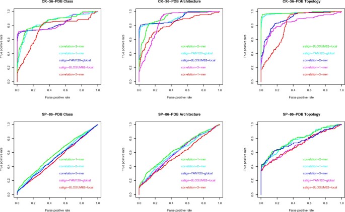
ROC curves for alignment and k -mer frequencies. ROC curves for global and local alignment and k-mer frequencies, one for each data set (CK-36-PDB and SP-86-PDB) and each classification task (class, architecture, topology).

Classification via algorithms: UPGMA and NJ
This set of experiments aims at establishing how well the dissimilarity matrices computed via UCD, NCD and CD, with different compressors, can be used for classification by two well known and widely available classification algorithms. We have chosen UPGMA [31] and NJ [32], two classic tree construction algorithms, as implemented in BioPerl [33]. In relation to the clustering literature [34], both can be considered as Hierarchical Methods. In fact, UPGMA is also known as Average Link Hierarchical Clustering. NJ does not seem to have a counterpart in the clustering literature, although it certainly belongs to the Hierarchical Clustering algorithmic paradigm.
In order to assess the performance of compression-based classification, via UPGMA and NJ under various compression algorithms, we have computed two external measures [34], the F-measure and the partition distance, against a gold standard. The relevant features of those two measures is presented in the Methods section.
For the classification of protein domains, we have taken as the gold standard the CATH classification [20], although we might have adopted the SCOP classification [35] instead and, as a matter of fact, there are ongoing efforts to combine both classifications of protein domains [36, 37]. In order to obtain a partitional clustering solution from the tree computed by UPGMA, we place in the same cluster all proteins that descend from the same level one ancestor in the UPGMA tree. Then, we can compute the F-measure by using this clustering solution and the gold standard division of proteins in groups according to CATH class. The same procedure is used for NJ.
On the other hand, the classification of species we have taken as the gold standard is the NCBI taxonomy [38]. In this case, we can simply compare the two trees computed by UPGMA and NJ against the NCBI taxonomy, via the partition distance. Again, we might have adopted any other classification of species instead such as, for instance, the global phylogeny of fully sequenced organisms of [39].
We first computed for each compression algorithm the UCD, NCD and CD dissimilarity measures over all pairs of elements in the data set, then obtained classification trees using UPGMA and NJ and finally, computed the F-measure between the clustering solution obtained from those classification trees and the corresponding gold standard, for the first five data sets. We used the partition distance for the last one, as mentioned already. We followed an analogous procedure in order to obtain results via the non-compressive methods, the only difference being the computation of the dissimilarity matrix. Tables 1, 2, 3, 4, 5, 6 report the results on the six different data sets for the compression based measures, whereas Table 7 summarizes the ones obtained using the standard methods.
The following conclusions can be drawn from the experiments, with reference to the open questions posed in the Background section:
-
1)
Question (A). In agreement with the ROC analysis, UCD and NCD are virtually indistinguishable. That is, once we have fixed the data set and compressor, the value of the F-measure or partition distance is quite close for UCD and NCD and in most cases better than CD.
-
2)
Question (B) UPGMA seems to take better advantage of the USM methodology with respect to NJ. Indeed, given a compressor, the values of the F-measure obtained via UPGMA is in most cases better than those obtained with NJ, by as much as 14 %, on the different representations of the CK-36 data set. On the SK-86 data sets, all compressors and classification algorithms did poorly. Analogous poor performance was obtained with the use of standard techniques, again indicating (see ROC analysis) that SK-86 proteins may be difficult to classify. On the AA-15-DNA data set, once the compressor is fixed, the difference in value of the partition distance is very limited (plus/minus 1) in most cases and large (a maximum of 7) in a few others. It is also worth pointing out that the best performing compression algorithms, with UPGMA and NJ, reach excellent values of the F-measure and partition distance (very close to a perfect classification) on the CK-36 data sets and on the AA-15-DNA data set.
-
3)
Question (C). The results of the ROC analysis are largely confirmed on the CK-36 and SK-86 data sets. In particular, the difference in performance, as measured by the F-measure, between "with memory" compressors and memoryless ones is of some significance only on the CK-36-PDB data set. As for the AA-15-DNA data set, there are a few things worth noting. Gencompress, the best performing compression algorithm for DNA sequences, is the best performer on that data set together with PPMd. However, PPMd is 10 times faster in compression speed (see Table 8) and twice as fast in decompression speed. Moreover, the difference between "with memory" and memoryless algorithms is substantial and there is, in fact, a clear separation in terms of the partition distance values for those two classes of algorithms. So, those results, together with the ones on the other data sets, indicate that "with memory" compressors are substantially better than memoryless compressors only on data sets where there is enough "structure", a property not shared by many data sets of biological relevance.
-
4)
Question (D). The results of the AUC analysis are largely confirmed here, again showing that the USM methodology has the same performance and limitations as more standard methods. In particular, PPMd together with UCD and UPGMA gives a value of the F-measure within 2% of the value obtained with standard methods. Again, this seems to indicate that the main advantage of the USM methodology with respect to existing ones is its scalability with data set size.
Compression performance
For completeness, we also report compression ratios on all data sets (Table 8) as well as compression and decompression times on some relevant data sets (Table 9).
Conclusion
Prior to this research, the USM methodology was perceived as adequate for analysis of biological data mainly because of its flexibility and scalability with data set size. In particular, it would be applicable to any biological data in textual format. That is, it would work well on data sets not necessarily consisting of genomic or proteomic sequences and even with large data sets. Moreover, only the best compression algorithms were recommended for use with the methodology, based on the intuitively appealing explanation that the better the compression guaranteed by a program, the better classification it would guarantee when used with USM. As the results in Table 8 show, memoryless compressors can guarantee compression results comparable to the ones of "with memory" compressors on biological data, even if they are, in general, bad compressors. So, they cannot be dismissed based only on that intuition, even more so since they are fast and use very little main memory. Our study adds to the state-of-the-art the following methodological conclusions and a recipe to use USM on biological data sets.
The USM methodology is worth using, even on data sets of size small enough to be processed by standard methods, including the ones based on alignments. It has the same advantages and limitations of the standard methods, i.e., data sets that can be classified well and others that are difficult to classify. Given that no similarity or dissimilarity measure is likely to be general enough to handle well all data sets, the USM methodology is a valid alternative to existing techniques. Moreover, because of their speed (see Table 9) and low memory requirements, memoryless compressors should be dismissed as not worthy only when the data sets have enough structure-something that should be evaluated using domain knowledge before applying the methodology to a data set.
In general, one of UCD or NCD should be used, in conjunction with UPGMA. As for compression algorithms, when very little is known about whether the data set has structure or not, PPMd and Gencompress are the algorithms likely to give the best results. When speed is important, Gzip is a valid alternative to both of them.
Methods
Kolmogorov Complexity and Information Theory: the Universal Similarity Metric and its compression-based approximations
The conditional Kolmogorov complexity K(x|y) of two strings x and y is the length of the shortest binary program P that computes x with input y [8, 40]. Thus, K(x|y) represents the minimal amount of information required to generate x by any effective computation when y is given as an input to the computation. The Kolmogorov complexity K (x) of a string x is defined as K(x|λ), where λ stands for the empty string. Given a string x, let x* denote the shortest binary program that produces x on an empty input; if there is more than one shortest program, x* is the first one in enumeration order. The Kolmogorov complexity K (x, y) of a pair of objects x and y is the length of the shortest binary program that produces x and y and a way to tell them apart. It is then possible to define the information distance ID (x, y) between two objects satisfying the following identity, up to logarithmic additive terms:
ID (x, y) = max {K (x|y), K (y|x)}
Equation (1) is the Kolmogorov complexity of describing object x, given y and vice versa. It can be shown to be a proper metric [41] and therefore, a distance function for strings. A major further advancement in Kolmogorov complexity-based distance functions has been obtained in [7], where
has been defined and properly denoted as the universal similarity metric. In fact, it is a metric, it is normalized and it is universal: a lower bound to, and therefore a refinement of, any distance function that one can define and compute.
It is well known that there is a relationship between Kolmogorov complexity of sequences and Shannon information theory [42]: the expected Kolmogorov complexity of a sequence x is asymptotically close to the entropy of the information source emitting x.
Such a fact is of great use in defining workable distance and similarity functions stemming from the theoretic setting outlined above. Indeed, Kolmogorov complexities are non-computable in the Turing sense, so the universal similarity metric must be approximated, via the entropy of the information source emitting x. However, it is very hard to infer the information source from the data. So, in order to approximate K (x), one resorts to compressive estimates of entropy.
Let C be a compression algorithm and C (x) (usually a binary string) its output on a string x. Let |C (x)|/|x| be its compression rate, i.e., the ratio of the lengths of the two strings. Usually, the compression rate of good compressors approaches the entropy of the information source emitting x [42]. While entropy establishes a lower bound on compression rates, it is not straightforward to measure entropy itself, as already pointed out. One empirical method inverts the relationship and estimates entropy by applying a provably good compressor to a sufficiently long, representative string. That is, the compression rate becomes a compressive estimate of entropy.
In conclusion, we must be satisfied by approximating K (x) by the length |C (x)|. Furthermore, since K (x, y) = K (xy) up to additive logarithmic precision [7], K (x, y) can be likewise approximated by the length |C (xy)| of the compression of the concatenation of x and y. Finally, and since K (x, y) = K (x) + K (y|x*) = K (y) + K (x|y*), again up to constant additive precision [8], the conditional complexity K (x|y*) is the limit approximation of |C (xy)| - |C (y)|, and K (y|x*) is the limit approximation of |C (yx)| - |C (x)|. This gives us our first dissimilarity function:
Furthermore, the authors of the USM methodology have devised compressive estimates of it: Namely,
Based on it, we consider
NCD (x, y) = min {NCD1 (x, y), NCD1 (y, x)}
Notice that this is a slight variation with respect to the original definition to make the function symmetric. Finally, in the realm of data mining and as an approximation of USM and independently in table compression applications, the following dissimilarity function was proposed:
Data sets
The Chew-Kedem data set consists of the following proteins:
alpha-beta 1aa900, 1chrA1, 1ct9A1, 1gnp00, 1qraA0, 2mnr01, 4enl01, 5p2100, 6q21A0, 6xia00.
mainly beta 1cd800, 1cdb00, 1ci5A0, 1hnf01, 1neu00, 1qa9A0, 1qfoA0.
mainly alpha 1ash00, 1babA0, 1babB0, 1cnpA0, 1eca00, 1flp00, 1hlb00, 1hlm00, 1ithA0, 1jhgA0, 1lh200, 1mba00, 1myt00, 2hbg00, 2lhb00, 2vhb00, 2vhbA0, 3sdhA0, 5mbn00.
Protein chain 2vhb00 appears twice in this data set, as 2vhb00 and 2vhbA0, in order to test whether the two chains are detected by compression-based classification methods to be identical (and thus clustered together) or not.
The Sierk-Pearson protein data set is as follows:
alpha-beta 1a1mA1, 1a2vA2, 1akn00, 1aqzB0, 1asyA2, 1atiA2, 1auq00, 1ax4A1, 1b0pA6, 1b2rA2, 1bcg00, 1bcmA1, 1bf5A4, 1bkcE0, 1bp7A0, 1c4kA2, 1cd2A0, 1cdg01, 1d0nA4, 1d4oA0, 1d7oA0, 1doi00, 1dy0A0, 1e2kB0, 1eccA1, 1fbnA0, 1gsoA3, 1mpyA2, 1obr00, 1p3801, 1pty00, 1qb7A0, 1qmvA0, 1urnA0, 1zfjA0, 2acy00, 2drpA1, 2nmtA2, 2reb01, 4mdhA2.
mainly beta 1a8d02, 1a8h02, 1aozA3, 1b8mB0, 1bf203, 1bjqB0, 1bqyA2, 1btkB0, 1c1zA5, 1cl7H0, 1d3sA0, 1danU0, 1dsyA0, 1dxmA0, 1et6A2, 1extB1, 1nfiC1, 1nukA0, 1otcA1, 1qdmA2, 1qe6D0, 1qfkL2, 1que01, 1rmg00, 1tmo04, 2tbvC0.
mainly alpha 1ad600, 1ao6A5, 1bbhA0, 1cnsA1, 1d2zD0, 1dat00, 1e12A0, 1eqzE0, 1gwxA0, 1hgu00, 1hlm00, 1jnk02, 1mmoD0, 1nubA0, 1quuA1, 1repC1, 1sw6A0, 1trrA0, 2hpdA0, 2mtaC0.
The Apostolico data set consists of the mitochondrial DNA complete genome of the following species:
Laurasiatheria blue whale (B. musculus), finback whale (B. physalus), white rhino (C. simum), horse (E. caballus), gray seal (H. grypus), harbor seal (P. vitulina).
Murinae house mouse (M. musculus), rat (R. norvegicus).
Hominoidea gorilla (G. gorilla), human (H. sapiens), gibbon (H. lar), pigmy chimpanzee (P. paniscus), chimpanzee (P. troglodytes), sumatran orangutan (P. pygmaeus abelii), orangutan (P. pygmaeus).
Algorithms
Compression algorithms
The compression algorithms we have used for the computation of the dissimilarity functions defined earlier, together with their parameter setting-a crucial and many times overlooked aspect of data compression-can be broadly divided into four groups. The first group consists of three state-of-the-art tools for general purpose compression.
Gzip and Bzip2 These are the well known compression tools based respectively on the classic Lempel-Ziv algorithm [43] and the bwt (Burrows-Wheeler transform) [44].
PPMd This algorithm, written by Dmitry Shkarin [45, 46], is the current state-of-the-art for PPM compression. In our tests we used it with four different context lengths (see below).
The algorithms in the second group are known as order zero-or memoryless-compressors since the codeword for a symbol only depends on its overall frequency (for Huffman Coding) or on its frequency in the already scanned part of the input (for Range and Arithmetic Coding).
Huffman An implementation of the classic two-pass Huffman coding scheme.
Ac Arithmetic coding algorithm as implemented in [47].
Rc Range coding algorithm. Range coding and arithmetic coding are based on similar concepts and achieve similar compression. We used the Range Coding implementation from [48].
The algorithms in the next group are all based on the bwt and have been implemented and tested in [49].
BwtMtfRleHuff and BwtRleHuff. The first of these algorithms consists in computing the bwt followed by Move-to-front encoding, followed by the run-length encoding, followed by Huffman coding (as implemented by algorithm Huffman). The algorithm BwtRleHuff is analogous to Huffman except that the Move-to-front encoding step is omitted.
BwtMtfRleAc and BwtRleAc are analogous respectively to BwtMtfRleHuff and BwtRleHuff, except that in the final step they use Arithmetic Coding (algorithm Ac) instead of Huffman coding.
BwtMtfRleRc and BwtRleRc are analogous respectively to BwtMtfRleHuff and BwtRleHuff, except that in the final step they use Range Coding (algorithm Rc) instead of Huffman Coding.
BwtWavelet computes the bwt of the input and compresses the resulting string using a wavelet tree encoder [50].
Finally, we used an algorithm specially designed for compressing DNA sequences.
Gencompress This is currently the best available algorithm to compress DNA sequences [51]. It makes clever use of approximate occurrences of substrings in DNA sequences to achieve good compression.
Range/arithmetic coding variants
The behavior of range and arithmetic coding depends on two parameters: MaxFreq and Increment. The ratio between these two values essentially controls how quickly the coding "adapts" to the new statistics. For range coding we set MaxFreq = 65, 536 (the largest possible value) and we experimented with three different values of Increment. Setting Increment = 256 we get a range coder with FAST adaptation, with Increment = 32 we get a range coder with MEDIUM adaptation and finally, setting Increment = 4 we get a range coder with SLOW adaptation. Similarly for arithmetic coding we set MaxFreq = 16, 383 (the largest possible value) and Increment equal to 64, 8, 1 to achieve respectively FAST, MEDIUM, and SLOW adaptation.
PPMd variants
The compressive power of PPMd is strictly related to the length of the contexts which are used for predicting the next symbol. In our experiments, we have used models (contexts) of length 2, 4, 8 and 16, and 256 Mb of working memory. Contexts of length 16 represent PPMd at its maximum strength. In the tables the number beside PPMd indicates the context length used.
Alignment and alignment-free algorithms
The alignment algorithms we have used are the global alignment algorithm of [52] with the PAM120 substitution scoring matrix [53], and the local alignment algorithm of [54] with the BLOSUM62 substitution scoring matrix [55], as implemented in the R package pairseqsim [56].
For alignment-free comparison, we have computed the linear correlation coefficient between the 20kdimensional vectors of k-mer frequencies [5, 15] for k = 1, 2, 3, using the R package seqinr [57].
Dissimilarity matrix construction algorithms
We have produced BioPerl scripts that take as input a set of files to be classified and a compression algorithm (together with all of its proper parameter settings) and that return a dissimilarity matrix. In particular, there is a preprocessing script that computes all the needed compression values in order to compute UCD, NCD and CD. In turn, there is a script corresponding to each of them that, given as input the results of the preprocessing step, produces the actual dissimilarity matrix. A detailed description of these scripts is given in the readme file at the supplementary material web site, at [1].
ROC curves and external measures
A ROC curve [58] is a plot of the true positive rate (the sensitivity) versus the false positive rate (one minus the specificity) for a binary classifier as the discrimination threshold changes. The AUC is a value ranging from 1 for a perfect classification, with 100% sensitivity (all true positives are found) to 0 for the worst possible classification, with 0% sensitivity (no true positive is found). A random classifier has an AUC value around 0.5. When plotted, the better the ROC curve follows the ordinate and then the abscissa line, the better the classification. The ROC curve of a random classifier, when plotted, is close to the diagonal. The F-measure [59] takes in input two classifications of objects, that is, two partitions of the same set of objects, and returns a value ranging from 0 for highest dissimilarity to 1 for identical classifications. The partition (or symmetric difference) distance [60, 61], takes in input the tree topologies of two alternative classifications of n species and returns a value ranging from 0 to 4n - 10. It is the number of clades in the two rooted trees that do not match and it is increasing with dissimilarity. When zero, it indicates isomorphic trees.
Experimental set-up and availability
All the experiments have been performed on a 64-bit AMD Athlon 2.2 GHz processor, 1 GB of main memory running both Windows XP and Linux. All software and data sets involved in our experimentation is available at the supplementary web site [1]. The software is given both as C++ code and Perl scripts and as executable code, tested on Linux (various versions – see supplementary material website), BSD Unix, Mac OS X and Windows operating systems.
References
Kolmogorov Library Supplementary Material Web Page. [http://www.math.unipa.it/~raffaele/kolmogorov/]
Kruskal J, Sankoff D, (Eds): Time Wraps, String Edits, and Macromolecules: The Theory and Practice of Sequence Comparison. 1983, Addison-Wesley
Waterman M: Introduction to Computational Biology. Maps, Sequences and Genomes. 1995, Chapman Hall
Gusfield D: Algorithms on Strings, Trees, and Sequences: Computer Science and Computational Biology. 1997, Cambridge University Press
Vinga S, Almeida J: Alignment-Free Sequence Comparison: A Review. Bioinformatics. 2003, 19 (4): 513-523.
Rissanen J: Modeling by shortest data description. Automatica. 1978, 14 (5): 465-471.
Li M, Chen X, Li X, Ma B, Vitányi PMB: The Similarity Metric. IEEE T. Inform. Theory. 2004, 50 (12): 3250-3264.
Li M, Vitányi PMB: An Introduction to Kolmogorov Complexity and its Applications. 1997, Springer-Verlag, 2
Cilibrasi R, Vitányi PMB: Clustering by Compression. IEEE T. Inform. Theory. 2005, 51 (4): 1523-1545.
Keogh E, Lonardi S, Rtanamahata C: Towards parameter-free data mining. Proc. 10th ACM SIGKDD Int. Conf. Knowledge Discovery and Data Mining, ACM. 2004, 206-215.
Buchsbaum AL, Caldwell DF, Church KW, Fowler GS, Muthukrishnan S: Engineering the Compression of Massive Tables: An Experimental Approach. Proc. 11th ACM-SIAM Symp. Discrete Algorithms. 2000, 175-184.
Buchsbaum AL, Fowler GS, Giancarlo R: Improving Table Compression with Combinatorial Optimization. J ACM. 2003, 50 (6): 825-851.
Krasnogor N, Pelta DA: Measuring the Similarity of Protein Structures by Means of the Universal Similarity Metric. Bioinformatics. 2004, 20 (7): 1015-1021.
Pelta D, Gonzales JR, Krasnogor N: Protein Structure Comparison through Fuzzy Contact Maps and the Universal Similarity Metric. Proc. 4th Conf. European Society for Fuzzy Logic and Technology and 11 Rencontres Francophones sur la Logique Floue et ses Applications (EUSFLAT-LFA, 2005). 2005, 1124-1129.
Gilbert D, Rosselló F, Valiente G, Veeramalai M: Alignment-Free Comparison of TOPS Strings. London Algorithmics and Stringology 2006. Edited by: Daykin J, Mohamed M, Steinhöfel K. 2007, College Publications, 8: 177-197.
Chew LP, Kedem K: Finding the Consensus Shape for a Protein Family. Algorithmica. 2003, 38: 115-129.
Sierk M, Person W: Sensitivity and Selectivity in Protein Structure Comparison. Protein Sci. 2004, 13 (3): 773-785.
Thiruv B, Quon G, Saldanha SA, Steipe B: Nh3D: A Reference Dataset of Non-Homologous Protein Structures. BMC Struct Biol. 2005, 5: 12-
Word JM, Lovell SC, LaBean TH, Taylor HC, Zalis ME, Presley BK, Richardson JS, Richardson DC: Visualizing and Quantifying Molecular Goodness-of-Fit: Small-Probe Contact Dots with Explicit Hydrogen Atoms. J Mol Biol. 1999, 285 (4): 1711-1733.
Pearl F: The CATH Domain Structure Database and Related Resources Gene3D and DHS Provide Comprehensive Domain Family Information for Genome Analysis. Nucleic Acids Res. 2005, 33 (D): D247-D251.
Pearson WR, Lipman DJ: Improved Tools for Biological Sequence Comparison. Proc Natl Acad Sci USA. 1998, 85 (8): 2444-2448.
Flores TP, Moss DM, Thornton JM: An Algorithm for Automatically Generating Protein Topology Cartoons. Protein Eng Des Sel. 1994, 7: 31-37.
Gilbert DR, Westhead DR, Nagano N, Thornton JM: Motif-Based Searching in TOPS Protein Topology Databases. Bioinformatics. 1999, 15: 317-326.
Westhead DR, Hutton DC, Thornton JM: An Atlas of Protein Topology Cartoons Available on the World Wide Web. Trends Biochem Sci. 1998, 23: 35-36.
Westhead DR, Slidel T, Flores T, Thornton JM: Protein Structural Topology: Automated Analysis and Diagrammatic Representations. Protein Sci. 1999, 8 (4): 897-904.
Kabsch W, Sander C: Dictionary of Protein Secondary Structure: Pattern Recognition of Hydrogen-Bonded and Geometrical Features. Biopolymers. 1983, 22 (12): 2577-2637.
Mauri F, Omnaas J, Davidson L, Whitfill C, Kitto GB: Amino acid sequence of a globin from the sea cucumber Caudina (Molpadia) arenicola. Biochimica et Biophysica Acta. 1991, 1078: 63-67.
McDonald GD, Davidson L, Kitto GB: Amino acid sequence of the coelomic C globin from the sea cucumber Caudina (Molpadia) arenicola. J Protein Chem. 1992, 11: 29-37.
Apostolico A, Comin M, Parida L: Mining, Compressing and Classifying with Extensible Motifs. Algorithms Mol Biol. 2006, 1: 4-
Sing T, Sander O, Beerenwinkel N, Lengauer T: ROCR: Visualizing Classifier Performance in R. Bioinformatics. 2005, 21 (20): 3940-3941.
Sneath PHA, Sokal RR: Numerical Taxonomy: The Principles and Practice of Numerical Classification. 1973, San Francisco: W. H. Freeman
Saitou N, Nei M: The Neighbor-Joining Method: A New Method for Reconstructing Phylogenetic Trees. Mol Biol Evol. 1987, 4 (4): 406-425.
Stajich JE: The BioPerl Toolkit: Perl Modules for the Life Sciences. Genome Res. 2002, 12 (10): 1611-1618. [http://www.bioperl.org]
Handl J, Knowles J, Kell DB: Computational Cluster Validation in Post-Genomic Data Analysis. Bioinformatics. 2005, 21 (15): 3201-3212.
Murzin AG, Brenner SE, Hubbard T, Chothia C: SCOP: A Structural Classification of Proteins Database for the Investigation of Sequences and Structures. J Mol Biol. 1995, 247 (4): 536-540.
Day R, Beck DA, Armen RS, Daggett V: A consensus view of fold space: Combining SCOP, CATH, and the Dali Domain Dictionary. Protein Sci. 2003, 12 (10): 2150-2160.
Hadley C, Jones DT: A Systematic Comparison of Protein Structure Classifications: SCOP, CATH and FSSP. Structure. 1999, 7 (9): 1099-1112.
Wheeler DL, Chappey C, Lash AE, Leipe DD, Madden TL, Schuler GD, Tatusova TA, Rapp BA: Database resources of the National Center for Biotechnology Information. Nucleic Acids Res. 2000, 28: 10-14. [http://www.ncbi.nlm.nih.gov/Taxonomy/]
Ciccarelli FD, Doerks T, von Mering C, Creevey CJ, Snel B, Bork P: Toward Automatic Reconstruction of a Highly Resolved Tree of Life. Science. 2006, 311 (5765): 1283-1287.
Kolmogorov AN: Three Approaches to the Quantitative Definition of Information. Probl Inform Transm. 1965, 1: 1-7.
Bennett CH, Gács P, Li M, Vitányi PMB, Zurek W: Information Distance. IEEE T. Inform. Theory. 1998, 44 (7): 1407-1423.
Cover TM, Thomas JA: Elements of Information Theory. 1990, Wiley
Ziv J, Lempel A: A universal algorithm for sequential data compression. IEEE T. Inform. Theory. 1977, 23 (3): 337-343.
Burrows M, Wheeler D: A block sorting lossless data compression algorithm. Tech. Rep. 124, Digital Equipment Corporation. 1994
Shkarin D: PPM: One step to practicality. IEEE Data Compression Conference, IEEE. 2002, 202-211.
Shkarin D: PPMd Compressor Ver. J. 2006, [http://www.compression.ru/ds/]
Witten IH, Neal RM, Cleary JG: Arithmetic coding for data compression. Commun ACM. 1987, 30 (6): 520-540.
Lundqvist M: Carryless Range Coding. 2006, [http://mikaellq.net/software.htm]
Ferragina P, Giancarlo R, Manzini G: The Myriad Virtues of Wavelet Trees. Proc. 33rd Int. Coll. Automata, Languages and Programming, of Lecture Notes in Computer Science. 2006, Berlin: Springer-Verlag, 4051: 561-572.
Grossi R, Gupta A, Vitter J: High-Order Entropy-Compressed Text Indexes. Proc. 14th Annual ACM-SIAM Symp. Discrete Algorithms, ACM. 2003, 841-850.
Chen X, Kwong S, Li M: A compression algorithm for DNA sequences. IEEE Engineering in Medicine and Biology Magazine. 2001, 20 (4): 61-66.
Needleman S, Wunsch C: A General Method applicable to the Search for Similarities in the Amino Acid Sequence of two Proteins. J Mol Biol. 1970, 48 (3): 443-453.
Altschul SF, Gish W, Miller W, Myers EW, Lipman DJ: Basic Local Alignment Search Tool. J Mol Biol. 1990, 215 (3): 403-410.
Smith TF, Waterman MS: Identification of Common Molecular Subsequences. J Mol Biol. 1981, 147: 195-197.
Henikoff S, Henikoff JG: Amino Acid Substitution Matrices from Protein Blocks. Proc Natl Acad Sci USA. 1992, 89 (22): 10915-10919.
Wolski W: pairseqsim: Pairwise Sequence Alignment and Scoring Algorithms for Global, Local and Overlap Alignment with Affine Gap Penalty. 2007, [http://www.bioconductor.org]
Charif D, Lobry JR: SeqinR 1.0–2: A Contributed Package to the R Project for Statistical Computing Devoted to Biological Sequences Retrieval and Analysis. Structural Approaches to Sequence Evolution: Molecules, Networks, Populations, Biological and Medical Physics, Biomedical Engineering. Edited by: Bastolla U, Porto M, Roman HE, Vendruscolo M. 2007, New York: Springer-Verlag
Lasko TA, Bhagwat JG, Zou KH, Ohno-Machado L: The Use of Receiver Operating Characteristic Curves in Biomedical Informatics. J Biomed Inform. 2005, 38: 404-415.
van Rijsbergen CJ: Information Retrieval. 1979, London: Butterworths, 2
Penny D, Hendy MD: The Use of Tree Comparison Metrics. Syst Zool. 1985, 34: 75-82.
Robinson DF, Foulds LR: Comparison of Weighted Labelled Trees. Proc. 6th Australian Conf. Combinatorial Mathematics, of Lecture Notes Mathematics. 1979, Berlin: Springer-Verlag, 748: 119-126.
Acknowledgements
The authors wish to thank Ming Li and Francesc Rosselló for their valuable advice and comments on compression based classification. PF was partially supported by Italian MIUR grants Italy-Israel FIRB "Pattern Discovery Algorithms in Discrete Structures, with Applications to Bioinformatics" and PRIN "MainStream MAssive INformation structures and dataSTREAMs". RG was partially supported by Italian MIUR grants PRIN "Metodi Combinatori ed Algoritmici per la Scoperta di Patterns in Biosequenze" and FIRB "Bioinformatica per la Genomica e la Proteomica" and Italy-Israel FIRB Project "Pattern Discovery Algorithms in Discrete Structures, with Applications to Bioinformatics". GM was partially supported by Italian MIUR Italy-Israel FIRB Project "Pattern Discovery Algorithms in Discrete Structures, with Applications to Bioinformatics". GV was partially supported by Spanish CICYT project TIN 2004-07925-C03-01 GRAMMARS, by Spanish DGES project MTM2006-07773 COMGRIO, and by EU project INTAS IT 04-77-7178.
Author information
Authors and Affiliations
Corresponding author
Additional information
Competing interests
The author(s) declare that they have no competing interests.
Authors' contributions
RG and GV conceived the method and prepared the manuscript. GV implemented part of the software and performed the ROC analysis and some of the experiments. VG implemented part of the software and performed most of the experiments. PF and GM contributed software for compression methods. All authors contributed to the discussion and have approved the final manuscript.
Authors’ original submitted files for images
Below are the links to the authors’ original submitted files for images.
Rights and permissions
Open Access This article is published under license to BioMed Central Ltd. This is an Open Access article is distributed under the terms of the Creative Commons Attribution License ( https://creativecommons.org/licenses/by/2.0 ), which permits unrestricted use, distribution, and reproduction in any medium, provided the original work is properly cited.
About this article
Cite this article
Ferragina, P., Giancarlo, R., Greco, V. et al. Compression-based classification of biological sequences and structures via the Universal Similarity Metric: experimental assessment. BMC Bioinformatics 8, 252 (2007). https://doi.org/10.1186/1471-2105-8-252
Received:
Accepted:
Published:
DOI: https://doi.org/10.1186/1471-2105-8-252