Abstract
Background
As a high-throughput technology that offers rapid quantification of multidimensional characteristics for millions of cells, flow cytometry (FCM) is widely used in health research, medical diagnosis and treatment, and vaccine development. Nevertheless, there is an increasing concern about the lack of appropriate software tools to provide an automated analysis platform to parallelize the high-throughput data-generation platform. Currently, to a large extent, FCM data analysis relies on the manual selection of sequential regions in 2-D graphical projections to extract the cell populations of interest. This is a time-consuming task that ignores the high-dimensionality of FCM data.
Results
In view of the aforementioned issues, we have developed an R package called flowClust to automate FCM analysis. flowClust implements a robust model-based clustering approach based on multivariate t mixture models with the Box-Cox transformation. The package provides the functionality to identify cell populations whilst simultaneously handling the commonly encountered issues of outlier identification and data transformation. It offers various tools to summarize and visualize a wealth of features of the clustering results. In addition, to ensure its convenience of use, flowClust has been adapted for the current FCM data format, and integrated with existing Bioconductor packages dedicated to FCM analysis.
Conclusion
flowClust addresses the issue of a dearth of software that helps automate FCM analysis with a sound theoretical foundation. It tends to give reproducible results, and helps reduce the significant subjectivity and human time cost encountered in FCM analysis. The package contributes to the cytometry community by offering an efficient, automated analysis platform which facilitates the active, ongoing technological advancement.
Background
Flow cytometry (FCM) is a high-throughput technology that offers rapid quantification of a set of physical and chemical characteristics for a large number of cells in a sample. FCM is widely used in health research and treatment for a variety of tasks, such as providing the counts of helper-T lymphocytes needed to monitor the course and treatment of HIV infection, in the diagnosis and monitoring of leukemia and lymphoma patients, the evaluation of peripheral blood hematopoietic stem cell grafts, and many other diseases [1–8]. The technology is also used in cross-matching organs for transplantation and in research involving stem cells, vaccine development, apoptosis, phagocytosis, and a wide range of cellular properties including phenotype, cytokine expression, and cell-cycle status [9–14].
Currently, FCM can be applied to analyze thousands of samples per day. Nevertheless, despite its widespread use, FCM has not reached its full potential due to the lack of an automated analysis platform to parallel the high-throughput data-generation platform. In contrast to the tremendous interest in the FCM technology, there is a dearth of statistical and bioinformatics tools to manage, analyze, present, and disseminate FCM data. There is considerable demand for the development of appropriate software tools, as manual analysis of individual samples is error-prone, non-reproducible, non-standardized, not open to re-evaluation, and requires an inordinate amount of time, making it a limiting aspect of the technology [1, 7, 15–21].
One core component of FCM analysis involves gating, the process of identifying cell populations that share a set of common properties or display a particular biological function. Currently, to a large extent, gating relies on the sequential application of a series of manually drawn gates (i.e., data filters) that define regions in 1- or 2-D graphical projections of FCM data. This process is manually time-consuming and subjective as researchers have traditionally relied on intuition rather than standardized statistical inference [7, 22, 23]. In addition, this process ignores the high-dimensionality of FCM data, which may convey more information than that provided by only looking at 1- or 2-D projections.
Recently, a suite of several R packages providing infrastructure for FCM analysis have been released though Bioconductor [24], an open source software development project for the analysis of genomic data. flowCore [25], the core package among them, provides data structures and basic manipulation of FCM data. flowViz [26] offers visualization tools, while flowQ provides quality control and quality assessment tools for FCM data. Finally, flowUtils provides utilities to deal with data import/export for flowCore. In spite of these low-level tools, there is still a dearth of software that helps automate FCM gating analysis with a sound theoretical foundation [15].
In view of these issues, based on a formal statistical clustering approach, we have developed the flowClust package (Additional file 1) to help resolve the current bottleneck. flowClust implements a robust model-based clustering approach [27–29] which extends the multivariate t mixture model with the Box-Cox transformation originally proposed in [30]. As a result of the extensions made, flowClust has included options allowing for a cluster-specific estimation of the Box-Cox transformation parameter and/or the degrees of freedom parameter; the Implementation section and the Results and Discussion section provide a detailed account of these extensions.
Implementation
The model
In statistics, model-based clustering [28, 29, 31, 32] is a popular unsupervised approach to look for homogeneous groups of observations. The most commonly used model-based clustering approach is based on finite Gaussian mixture models, which have been shown to give good results in various applied fields [28, 29, 33, 34]. However, Gaussian mixture models might give poor representations of clusters in the presence of outliers, or when the clusters are far from elliptical in shape, phenomena commonly observed in FCM data. In view of this, we have proposed in [30] an approach based on t mixture models [27, 28] with the Box-Cox transformation to handle these two issues simultaneously. Formally, given independent p-dimensional multivariate observations y1, y2,...,y n , and denoting by Ψ the collection of all unknown parameters, the likelihood for a mixture model with G components is

where w
g
is the probability that an observation belongs to the g-th component, and φ
p
(·|μ
g
, Σ
g
, ν
g
) is the p-dimensional multivariate t density with mean μ
g
(ν
g
> 1), covariance matrix ν
g
(ν
g
- 2)-1 Σ
g
(ν
g
> 2) and ν
g
degrees of freedom.  is the value obtained upon transforming y
i
with the Box-Cox parameter λ
g
; the transformation used is a variant of the original Box-Cox transformation which is also defined for negative-valued data [35]. Finally,
  is the Jacobian induced by the transformation. Please refer to [30] for a detailed account of an Expectation-Maximization (EM) algorithm [36] for the simultaneous estimation of all unknown parameters Ψ = (Ψ1,...,Ψ
G
) where Ψ
g
= (w
g
, μ
g
, Σ
g
, ν
g
, λ
g
).
The EM algorithm needs to be initialized. By default, random partitioning is performed 10 times in parallel, and the one delivering the highest likelihood value after a few EM runs will be selected as the initial configuration for the eventual EM algorithm.
Note that, in the model originally proposed in [30], the Box-Cox parameter λ is set common to all components of the mixture, and the degrees of freedom parameter ν is fixed at a predetermined common value. In the latest development of our software, we have generalized the model such that ν may also be estimated, and both λ and ν are allowed to be component-specific, as reflected in Equation (1).
When the number of clusters is unknown, we use the Bayesian Information Criterion (BIC) [37], which gives good results in the context of mixture models [29, 38].
The package
With the aforementioned theoretical basis, we have developed flowClust, an R package to conduct an automated FCM gating analysis and produce visualizations for the results. Its source code is written in C for optimal utilization of system resources and makes use of the Basic Linear Algebra Subprograms (BLAS) library, which facilitates multithreaded processes when an optimized library is provided.
flowClust is released through Bioconductor [24], along with those R packages mentioned in the Background section. The GNU Scientific Library (GSL) is needed for successful installation of flowClust. Please refer to the vignette that comes with flowClust for details about installation; Windows users may also consult the README file included in the package for procedures of linking GSL to R.
The package adopts a formal object-oriented programming discipline, making use of the S4 system [39] to define classes and methods. The core function, flowClust, implements the clustering methodology and returns an object of class flowClust. A flowClust object stores essential information related to the clustering result which can be retrieved through various methods such as summary, Map, getEstimates, etc. To visualize the clustering results, the plot and hist methods can be applied to produce scatterplots, contour/image plots and histograms.
To enhance communications with other Bioconductor packages designed for the cytometry community, flowClust has been built with the aim of being highly integrated with flowCore. Methods in flowClust can be directly applied on a flowFrame, the standard R implementation of a Flow Cytometry Standard (FCS) file defined in flowCore; FCS is the typical storage mode for FCM data. Another step towards integration is to overload basic filtering methods defined in flowCore (e.g., filter, %in%, Subset and split) in order to provide similar functionality for classes defined in flowClust.
Results and discussion
Analysis of real FCM data
In this section, we illustrate how to use flowClust to conduct an automated gating analysis of real FCM data. For demonstration, we use the graft-versus-host disease (GvHD) data (Additional file 2) [40]. The data are stored in FCS files, and consist of measurements of four fluorescently conjugated antibodies, namely, anti-CD4, anti-CD8β, anti-CD3 and anti-CD8, in addition to the forward scatter and sideward scatter parameters. One objective of the gating analysis is to look for the CD3+CD4+CD8β+ cell population, a distinctive feature found in GvHD-positive samples. We have adopted a two-stage strategy [30]: we first cluster the data by using the two scatter parameters to identify basic cell populations, and then perform clustering on the population of interest using all fluorescence parameters.
At the initial stage, we extract the lymphocyte population using the forward scatter (FSC-H) and sideward scatter (SSC-H) parameters:
GvHD <- read.FCS("B07", trans = FALSE)
res1 <- flowClust(GvHD, varNames = c("FSC-H", "SSC-H"), K = 1:8)
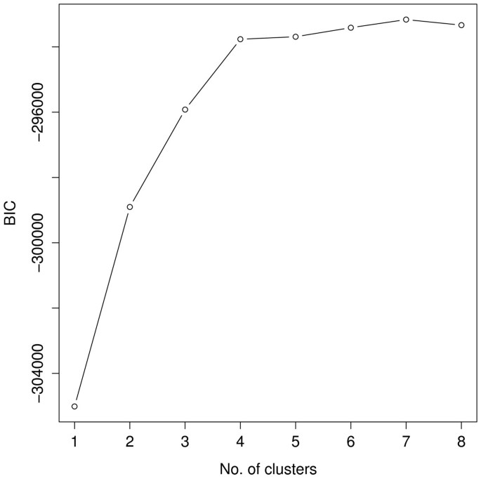
To estimate the number of clusters, we run flowClust on the data repetitively with K = 1 up to K = 8 clusters in turn, and apply the BIC to guide the choice. Values of the BIC can be retrieved through the criterion method. Figure 1 shows that the BIC curve remains relatively flat beyond four clusters. We therefore choose the model with four clusters. Below is a summary of the corresponding clustering result.
** Experiment Information **
Experiment name: Flow Experiment
Variables used: FSC-H SSC-H
** Clustering Summary **
Number of clusters: 4
Proportions: 0.1779686 0.1622115 0.3882043 0.2716157
** Transformation Parameter **
lambda: 0.1126388
** Information Criteria **
Log likelihood: -146769.5
BIC: -293765.9
ICL: -300546.2
** Data Quality **
Number of points filtered from above: 168 (1.31%)
Number of points filtered from below: 0 (0%)
Rule of identifying outliers: 90% quantile
Number of outliers: 506 (3.93%)
Uncertainty summary:
Min. 1st Qu. Median Mean 3rd Qu. Max. NA's
9.941e-04 1.211e-02 3.512e-02 8.787e-02 1.070e-01 6.531e-01 1.680e+02
The estimate of the Box-Cox parameter λ is 0.11, implying a transformation close to a logarithmic one (λ = 0).
Note that, by default, flowClust selects the same transformation for all clusters. We have also enabled the option of estimating the Box-Cox parameter λ for each cluster. For instance, if a user finds the shapes of the clusters significantly deviate from one another and opts for a different transformation for each cluster, he may write the following line of code:
flowClust(GvHD, varNames = c("FSC-H", "SSC-H"), K = 4, trans = 2)
The trans argument acts as a switch to govern how λ is handled: fixed at a predetermined value (trans = 0), estimated and set common to all clusters (trans = 1), or estimated for each cluster (trans = 2). Incidentally, the option of estimating the degrees of freedom parameter ν has also been made available, either common to all clusters or specific to each of them. The nu.est argument is the corresponding switch and takes a similar interpretation to trans. Such an option of estimating ν further fine-tunes the model-fitting process such that the fitted model can reflect the data-specific level of abundance of outliers. To compare the models adopting a different combination of these options, one may make use of the BIC again. See Additional file 3 for a graph with two BIC curves corresponding to the default setting (common λ) and the setting with cluster-specific λ, respectively. Little difference in the BIC values between the two settings can be observed. In accordance with the principle of parsimony in Statistics which favors a simpler model, we opt for the default setting here.
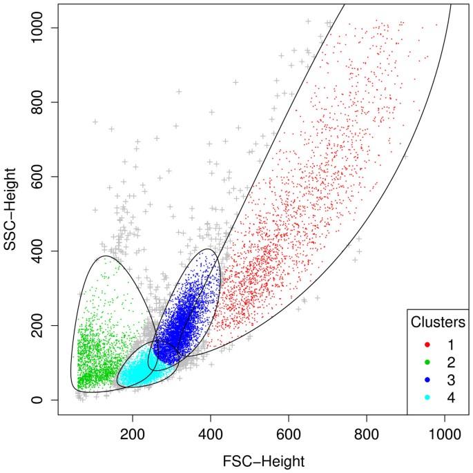
Graphical functionalities are available to users for visualizing a wealth of features of the clustering results, including the cluster assignment, outliers, and the size and shape of the clusters. Figure 2 is a scatterplot showing the cluster assignment of points upon the removal of outliers. Outliers are shown in grey with the + symbols. The black solid lines represent the 90% quantile region of the clusters which defines the cluster boundaries. The summary shown above states that the default rule used to identify outliers is 90% quantile, which means that a point outside the 90% quantile region of the cluster to which it is assigned will be called an outlier. In most applications, the default rule should be appropriate for identifying outliers. In case a user wants finer control and would like to specify a different rule, he may apply the ruleOutliers replacement method:
A scatterplot revealing the cluster assignment in the first-stage analysis. Clusters 1, 3 and 4 correspond to the lymphocyte population, while cluster 2 is referred to as the dead cell population. The black solid lines represent the 90% quantile region of the clusters which define the cluster boundaries. Points outside the boundary of the cluster to which they are assigned are called outliers and marked with "+".
ruleOutliers(res1[[4]]) <- list(level = 0.95)
See Additional file 4 for the corresponding summary. As shown in the summary, this rule is more stringent than the 90% quantile rule: 133 points (1.03%) are now called outliers, as opposed to 506 points (3.93%) in the default rule.
Clusters 1, 3 and 4 in Figure 2 correspond to the lymphocyte population defined with a manual gating strategy adopted in [40]. We then extract these three clusters to proceed with the second-stage analysis:
GvHD2 <- split(GvHD, res1[[4]], population = list(lymphocyte = c(1,3,4), deadcells = 2))
The subsetting method split allows us to split the data into several flowFrames representing the different cell populations. To extract the lymphocyte population (clusters 1, 3 and 4), we may type GvHD2$lymphocyte or GvHD2[[1]], which is a flowFrame. By default, split removes outliers upon extraction. The deadcells = 2 list element is included above for demonstration purpose; it is needed only if we want to extract the dead cell population (cluster 2), too.
In the second-stage analysis, in order to fully utilize the multidimensionality of FCM data we cluster the lymphocyte population using all the four fluorescence parameters, namely, anti-CD4 (FL1-H), anti-CD8β (FL2-H), anti-CD3 (FL3-H) and anti-CD8 (FL4-H), at once:
res2 <- flowClust(GvHD2$lymphocyte, varNames = c("FL1-H", "FL2-H", "FL3-H", "FL4-H"), K = 1:15)
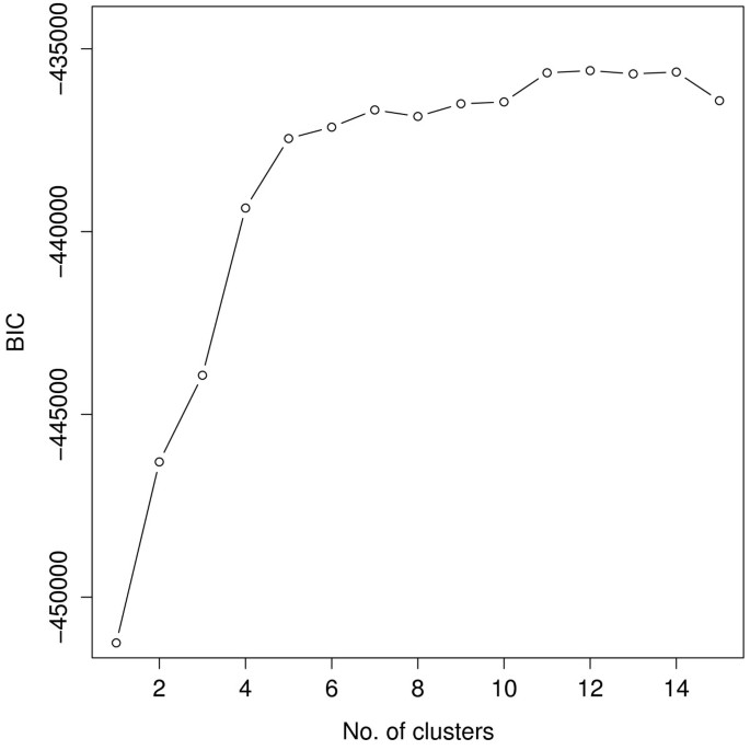
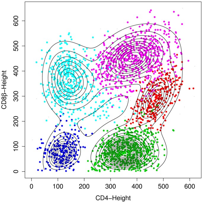
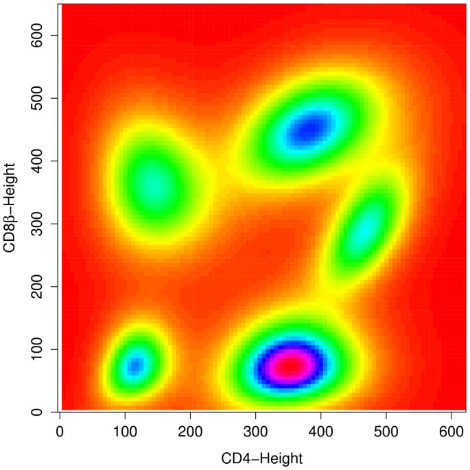
The BIC curve remains relatively flat beyond 11 clusters (Figure 3), suggesting that the model with 11 clusters provides a good fit. Figure 4 shows a contour plot superimposed on a scatterplot of CD8β against CD4 for the sub-population of CD3-stained cells, which were selected based on a threshold obtained from a negative control sample [40]. We can easily identify from it the red and purple clusters at the upper right as the CD3+CD4+CD8β+ cell population. A corresponding image plot is given by Figure 5. Also, see Additional file 5 for the code used to produce all the plots shown in this article.
The example above shows how an FCM analysis is conducted with the aid of flowClust. When the number of cell populations is not known in advance, and the BIC values are relatively close over a range of the possible number of clusters, the researcher may be presented with a set of possible solutions instead of a clear-cut single one. In such a case, the level of automation may be undermined as the researcher may need to select the best one based on his expertise. We acknowledge that more effort is needed to extend our proposed methodology towards a higher level of automation. Currently, we are working on an approach which successively merges the clusters in the solution as suggested by the BIC using some entropy criterion to give a more reasonable estimate of the number of clusters.
Integration with flowCore
As introduced in the Background section, flowClust has been built in a way such that it is highly integrated with the flowCore package. The core function flowClust which performs the clustering operation may be replaced by a call to the constructor tmixFilter creating a filter object similar to the ones used in other gating or filtering operations found in flowCore (e.g., rectangleGate, norm2Filter, kmeansFilter). As an example, the code
res1 <- flowClust(GvHD, varNames = c("FSC-H", "SSC-H"), K = 1:8)
used in the first-stage analysis of the GvHD data may be replaced by:
s1filter <- tmixFilter("lymphocyte", c("FSC-H", "SSC-H"), K = 1:8)
res1f <- filter(GvHD, s1filter)
The use of a dedicated tmixFilter-class object separates the task of specifying the settings (tmixFilter) from the actual filtering operation (filter), facilitating the common scenario in FCM gating analysis that filtering with the same settings is performed upon a large number of data files. The filter method returns a list object res1f with elements each of class tmixFilterResult, which directly extends the filterResult class defined in flowCore. Users may apply various subsetting operations defined for the filterResult class in a similar fashion on a tmixFilterResult object. For instance,
Subset(GvHD [, c("FSC-H", "SSC-H")], res1f[[4]])
outputs a flowFrame that is the subset of the GvHD data upon the removal of outliers, consisting of the two selected parameters, FSC-H and SSC-H, only. Another example is given by the split method introduced earlier in this section.
We realize that occasionally a researcher may opt to combine the use of flowClust with filtering operations in flowCore to define the whole sequence of an FCM gating analysis. To enable the exchange of results between the two packages, filters created by tmixFilter may be treated like those from flowCore; users of flowCore will find that filter operators, namely, &, |, ! and %subset%, also work in the flowClust package. For instance, suppose the researcher is interested in clustering the CD3+ cell population which he defines by constructing an interval gate with the lower end-point at 270 on the CD3 parameter. He may use the following code to perform the analysis:
rectGate <- rectangleGate(filterId="CD3+", "FL3-H" =c(270, Inf))
s2filter <- tmixFilter("s2filter", c("FL1-H", "FL2-H", "FL3-H", "FL4-H"), K = 5)
res2f <- filter(GvHD2$lymphocyte, s2filter %subset% rectGate)
The constructors rectangleGate and tmixFilter create two filter objects storing the settings of the interval gate and flowClust, respectively. When the last line of code is run, the interval gate will first be applied to the GvHD data. flowClust is then performed on a subset of the GvHD data contained by the interval gate.
Conclusion
flowClust is an R package dedicated to FCM gating analysis, addressing the increasing demand for software capable of processing and analyzing the voluminous amount of FCM data efficiently via an objective, reproducible and automated means. The package implements a statistical clustering approach using multivariate t mixture models with the Box-Cox transformation [30], and provides tools to summarize and visualize results of the analysis. The statistical model underlying flowClust extends the one originally proposed in [30]. The extensions have included modeling options allowing for a cluster-specific estimation of the Box-Cox parameter λ and the degrees of freedom parameter ν. The package contributes to the cytometry community by offering an efficient, automated analysis platform which facilitates the active, ongoing technological advancement.
Availability and requirements
Project name: flowClust
Project homepage: http://bioconductor.org
Operating systems: Platform independent
Programming language: C, R
Other requirements: GSL, R, Bioconductor
License: Artistic 2.0
Any restrictions to use by non-academics: flowClust depends on the mclust software, the use of which needs to abide by the terms stated in http://www.stat.washington.edu/mclust/license.txt.
References
Braylan RC: Impact of flow cytometry on the diagnosis and characterization of lymphomas, chronic lymphoproliferative disorders and plasma cell neoplasias. Cytometry A 2004, 58A: 57–61. 10.1002/cyto.a.10101
Hengel RL, Nicholson JK: An update on the use of flow cytometry in HIV infection and AIDS. Clin Lab Med 2001, 21(4):841–856.
Illoh OC: Current applications of flow cytometry in the diagnosis of primary immunodeficiency diseases. Arch Pathol Lab Med 2004, 128: 23–31.
Kiechle FL, Holland-Staley CA: Genomics, transcriptomics, proteomics, and numbers. Arch Pathol Lab Med 2003, 127(9):1089–1097.
Mandy FF: Twenty-five years of clinical flow cytometry: AIDS accelerated global instrument distribution. Cytometry A 2004, 58A: 55–56. 10.1002/cyto.a.10102
Orfao A, Ortuno F, de Santiago M, Lopez A, San Miguel J: Immunophenotyping of acute leukemias and myelodysplastic syndromes. Cytometry A 2004, 58A: 62–71. 10.1002/cyto.a.10104
Bagwell CB: DNA histogram analysis for node-negative breast cancer. Cytometry A 2004, 58A: 76–78. 10.1002/cyto.a.90004
Keeney M, Gratama JW, Sutherland DR: Critical role of flow cytometry in evaluating peripheral blood hematopoietic stem cell grafts. Cytometry A 2004, 58A: 72–75. 10.1002/cyto.a.10103
Krutzik PO, Irish JM, Nolan GP, Perez OD: Analysis of protein phosphorylation and cellular signaling events by flow cytometry: techniques and clinical applications. Clin Immunol 2004, 110(3):206–221. 10.1016/j.clim.2003.11.009
Maecker H, Maino V: Flow cytometric analysis of cytokines. 6th edition. Washington, DC: ASM Press. Manual of Clinical Laboratory Immunology; 2002.
Pozarowski P, Darzynkiewicz Z: Analysis of cell cycle by flow cytometry. Methods Mol Biol 2004, 281: 301–312.
Pala P, Hussell T, Openshaw PJ: Flow cytometric measurement of intracellular cytokines. J Immunol Methods 2000, 243(1–2):107–124. 10.1016/S0022-1759(00)00230-1
Vermes I, Haanen C, Reutelingsperger C: Flow cytometry of apoptotic cell death. J Immunol Methods 2000, 243(1–2):167–190. 10.1016/S0022-1759(00)00233-7
Lehmann AK, Sornes S, Halstensen A: Phagocytosis: measurement by flow cytometry. J Immunol Methods 2000, 243(1–2):229–242. 10.1016/S0022-1759(00)00237-4
Lizard G: Flow cytometry analyses and bioinformatics: Interest in new softwares to optimize novel technologies and to favor the emergence of innovative concepts in cell research. Cytometry A 2007, 71A: 646–647. 10.1002/cyto.a.20444
de Rosa SC, Brenchley JM, Roederer M: Beyond six colors: a new era in flow cytometry. Nat Med 2003, 9: 112–117. 10.1038/nm0103-112
Redelman D: CytometryML. Cytometry A 2004, 62A: 70–73. 10.1002/cyto.a.10093
Roederer M, Treister A, Moore W, Herzenberg LA: Probability binning comparison: a metric for quantitating univariate distribution differences. Cytometry 2001, 45(1):37–46. 10.1002/1097-0320(20010901)45:1<37::AID-CYTO1142>3.0.CO;2-E
Roederer M, Moore W, Treister A, Hardy RR, Herzenberg LA: Probability binning comparison: a metric for quantitating multivariate distribution differences. Cytometry 2001, 45(1):47–55. 10.1002/1097-0320(20010901)45:1<47::AID-CYTO1143>3.0.CO;2-A
Tzircotis G, Thorne RF, Isacke CM: A new spreadsheet method for the analysis of bivariate flow cytometric data. BMC Cell Biol 2004, 5: 10. 10.1186/1471-2121-5-10
Spidlen J, Gentleman RC, Haaland PD, Langille M, Le Meur N, Ochs MF, Schmitt C, Smith CA, Treister AS, Brinkman RR, et al.: Data standards for flow cytometry. OMICS 2006, 10(2):209–214. 10.1089/omi.2006.10.209
Suni MA, Dunn HS, Orr PL, de Laat R, Sinclair E, Ghanekar SA, Bredt BM, Dunne JF, Maino VC, Maecker HT: Performance of plate-based cytokine flow cytometry with automated data analysis. BMC Immunol 2003, 4: 9. 10.1186/1471-2172-4-9
Parks DR: Data processing and analysis: Data management. In Current Protocols in Cytometry. Volume chap. 10. New York: John Wiley & Sons, Inc.; 1997:10.1.1–10.1.6.
Gentleman RC, Carey VJ, Bates DM, Bolstad B, Dettling M, Dudoit S, Ellis B, Gautier L, Ge Y, Gentry J, Hornik K, Hothorn T, Huber W, Iacus S, Irizarry R, Leisch F, Li C, Maechler M, Rossini AJ, Sawitzki G, Smith C, Smyth G, Tierney L, Yang JYH, Zhang J: Bioconductor: Open software development for computational biology and bioinformatics. Genome Biol 2004, 5(10):R80. 10.1186/gb-2004-5-10-r80
Hahne F, Le Meur N, Brinkman R, Ellis B, Haaland P, Sarkar D, Spidlen J, Strain E, Gentleman R: flowCore: A Bioconductor software package for high throughput flow cytometry data analysis. BMC Bioinformatics 2008, 10: 106. 10.1186/1471-2105-10-106
Sarkar D, Le Meur N, Gentleman R: Using flowViz to visualize flow cytometry data. Bioinformatics 2008, 24(6):878–879. 10.1093/bioinformatics/btn021
Peel D, McLachlan GJ: Robust mixture modelling using the t distribution. Stat Comput 2000, 10(4):339–348. 10.1023/A:1008981510081
McLachlan G, Peel D: Finite Mixture Models. Wiley Series in Probability and Statistics: Applied Probability and Statistics, New York: Wiley-Interscience; 2000.
Fraley C, Raftery AE: Model-based clustering, discriminant analysis, and density estimation. J Amer Statist Assoc 2002, 97(458):611–631. 10.1198/016214502760047131
Lo K, Brinkman RR, Gottardo R: Automated gating of flow cytometry data via robust model-based clustering. Cytometry A 2008, 73(4):321–332.
Titterington DM, Smith AFM, Makov UE: Statistical Analysis of Finite Mixture Distributions. Chichester, UK: John Wiley & Sons; 1985.
McLachlan GJ, Basford KE: Mixture Models: Inference and Applications to Clustering. New York, NY: Marcel Dekker Inc; 1988.
Banfield JD, Raftery AE: Model-based Gaussian and Non-Gaussian Clustering. Biometrics 1993, 49: 803–821. 10.2307/2532201
Fraley C, Raftery AE: MCLUST Version 3 for R: Normal Mixture Modeling and Model-Based Clustering. In Technical Report. Department of Statistics, University of Washington; 2006.
Bickel PJ, Doksum KA: An analysis of transformations revisited. J Amer Statist Assoc 1981, 76(374):296–311. 10.2307/2287831
Dempster AP, Laird NM, Rubin DB: Maximum likelihood from incomplete data via the EM algorithm. J R Statist Soc B 1977, 39: 1–22.
Schwarz G: Estimating the Dimension of a Model. Ann Statist 1978, 6: 461–464. 10.1214/aos/1176344136
Fraley C, Raftery AE: How many clusters? Which clustering method? Answers via model-based cluster analysis. Comput J 1998, 41(8):578–588. 10.1093/comjnl/41.8.578
Chambers JM: Programming with Data: A Guide to the S Language. New York, NY: Springer; 2004.
Brinkman RR, Gasparetto M, Lee SJJ, Ribickas A, Perkins J, Janssen W, Smiley R, Smith C: High-content flow cytometry and temporal data analysis for defining a cellular signature of Graft-versus-Host disease. Biol Blood Marrow Transplant 2007, 13(6):691–700. 10.1016/j.bbmt.2007.02.002
Acknowledgements
The authors thank Martin Morgan, Patrick Aboyoun and Marc Carlson for their advice on the technical issues of building the flowClust package, and the two reviewers for suggestions that improved an earlier draft of the article. This work was supported by the NIH grants EB005034 and EB008400, and by the Michael Smith Foundation for Health Research.
Author information
Authors and Affiliations
Corresponding author
Additional information
Authors' contributions
KL and RG developed the methodology and software, and performed the analyses. FH participated in the development of the software. RRB and RG conceived of the study, and participated in its design and coordination. FH, RRB and RG helped KL draft the manuscript. All authors read and approved the final manuscript.
Electronic supplementary material
12859_2009_2875_MOESM1_ESM.zip
Additional file 1: A copy of the flowClust package. The zip file contains the source code of the flowClust package (version 2.2.0) as a gzipped tarball for direct installation into R from a command-line interface. This current release is also available from Bioconductor at http://bioconductor.org/packages/2.4/bioc/html/flowClust.html. (ZIP 262 KB)
12859_2009_2875_MOESM2_ESM.zip
Additional file 2: A copy of the GvHD data file used in this article. The zip file contains the data file in FCS format used in the GvHD analysis. Interested readers may go to http://www.ficcs.org/software.html#Data_Files for a complete set of data files for the GvHD study [40]. (ZIP 129 KB)
12859_2009_2875_MOESM3_ESM.pdf
Additional file 3: A graph with two BIC curves corresponding to the settings with a common λ and cluster-specific λ respectively for the first-stage cluster analysis. Little difference in the BIC values between the two settings is observed. In accordance with the principle of parsimony which favors a simpler model, we opt for the default setting here. (PDF 5 KB)
12859_2009_2875_MOESM4_ESM.txt
Additional file 4: Result summary of the first-stage analysis with four clusters of the GvHD data. The rule used to identify outliers is 95% quantile. 133 points (1.03%) are called outliers. (TXT 688 bytes)
12859_2009_2875_MOESM5_ESM.r
Additional file 5: Code to produce the plots in this article. R code to produce the plots in the GvHD analysis. (R 723 bytes)
Authors’ original submitted files for images
Below are the links to the authors’ original submitted files for images.
Rights and permissions
This article is published under license to BioMed Central Ltd. This is an Open Access article distributed under the terms of the Creative Commons Attribution License (http://creativecommons.org/licenses/by/2.0), which permits unrestricted use, distribution, and reproduction in any medium, provided the original work is properly cited.
About this article
Cite this article
Lo, K., Hahne, F., Brinkman, R.R. et al. flowClust: a Bioconductor package for automated gating of flow cytometry data. BMC Bioinformatics 10, 145 (2009). https://doi.org/10.1186/1471-2105-10-145
Received:
Accepted:
Published:
DOI: https://doi.org/10.1186/1471-2105-10-145


