
Abstract
In this article, some inequalities on convolution equations are presented firstly. The mean square stability of the zero solution of the impulsive stochastic Volterra equation is studied by using obtained inequalities on Liapunov function, including mean square exponential and non-exponential asymptotic stability. Several sufficient conditions for the mean square stability are presented. Results in this article indicate that not only the impulse intensity but also the time of impulse can influence the stability of the systems. At last, an example is given to show application of some obtained results.
Mathematics classification Primary(2000): 60H10, 60F15, 60J70, 34F05.
1 Introduction
Study on the stability of stochastic differential equations has gained lots of attention over the last years. The results and methods have been improved from time to time. Very recently, Taniguchi [1] studied the exponential stability for stochastic delay partial differential equations by use of the energy method which overcomes the difficulty of constructing the Liapunov functional on delay differential equations. Wan and Duan [2] extended the result of Taniguchi [1] to be applied to more general stochastic partial differential equations with memory. Another important method is about the fixed-point theory. It was first used to consider the exponential stability for stochastic partial differential equations with delays by Luo [3], where the conditions do not require the monotone decreasing behavior of the delays. This method also employed in Sakthivel and Luo [4, 5] to study the asymptotic stability of the nonlinear impulsive stochastic differential equations and the impulsive stochastic partial differential equations with infinite delays.
On considering Volterra equations, there is a significant literature devoted to the asymptotic stability of the zero solutions of Volterra integro-differential equations. In the known literature, the properties of linear scalar Voterra equation play an important role. The equation is

where the kernel k(t) is continuous, integrable and of a single sign. Brauer [6] showed that the solution could not be stable if  , Burton and Mahfoud [7] proved the zero solution is asymptotically stable if
  , Kordonis and Philos [8] discussed the stability of the solution under condition
  . Therefore, a necessary condition for
  for all solutions is that
  . About exponential asymptotic stability, Murakami [9] showed that the uniform asymptotic stability and the exponential asymptotic stability of the zero solution of this equation are equivalent if and only if
  for some γ > 0. Hence if it fails to hold, a uniformly asymptotically stable solution cannot be exponentially asymptotically stable. Some deeper related work on deterministic equations by Appleby can be found in [10–12], including the so-called "non-exponential decay rate" and "subexponential solution". Mao [13] investigated the mean square stability of the generalized equation

On some special stochastic volterra equations without impulse, we highlight here the contribution of Appely [14–19]. However real-world systems can be modeled to include random effects, including stochastic perturbations and impulses. It is natural to ask how the presence of such random effects can influence the stability of the systems. Based on the generalized equation [13], in this article, we consider the effect of the impulse intensity and the impulse time on the mean square exponential and non-exponential asymptotic stability of impulsive stochastic Volterra equation

for all i ∈ N = {0, 1, 2, ·····} by using Liapunov function, which show that both the presence of impulses and the time of the presence can influence the stability of the systems. By choosing the impulse intensity and the impulse time, We find that is not necessary condition for the exponential asymptotic stability.
The article is organized as follows: some preliminary notations and useful lemmas are given in Sect. 2. Then, sufficient conditions of the mean square exponential asymptotic stability are shown in the first part of Sect. 3, and the second part mainly deals with the mean square non-exponential asymptotic stability of the solution. Finally, an example is given.
2 Preliminary notes
Let {τ
i
, i = 1, 2,...} be a series of numbers such that t0 = τ0 < ···< τk < τk+1< ··· and  . We denote R+ = [0, +1). Consider the impulsive stochastic Volterra equations

where D
i
= (τI, τi+1) for all i ∈ N. f(t, x, y) : R+ × Rn × Rn → Rn, g(t, x, y) : R+ × Rn × Rn → Rn. ξ
i
= τ
i
- τi-1,  with respect to probability distribution for all i = 1, 2,.... I
i
(t, x) : R+ × Rn → Rn. F (t) and G(t) are both continuous and integrable matrix-valued functions on R+. B(t) is standard n-dimensional Brownian motion on a complete filtered probability space Ω, F, (FB (t)) t ≥ 0, P), where the filtration is defined as F B(t) = σ (B(s) : 0 ≤ s ≤ t). Almost sure events are Palmost sure in this article denoted by "a.s.". Suppose f(t, 0, y) = 0, g(t, 0, y) = 0 and I
i
(t, 0) = 0 for t > t0, then x(t) ≡ 0 is the solution of (1), which is called zero solution of (1). In this article, we always assume there exists a unique stochastic process satisfying (1), and assume all solutions of (1) are continuous on the left and limitable on the right. We further recall the various standard notions of stability of the zero solution required.
with respect to probability distribution for all i = 1, 2,.... I
i
(t, x) : R+ × Rn → Rn. F (t) and G(t) are both continuous and integrable matrix-valued functions on R+. B(t) is standard n-dimensional Brownian motion on a complete filtered probability space Ω, F, (FB (t)) t ≥ 0, P), where the filtration is defined as F B(t) = σ (B(s) : 0 ≤ s ≤ t). Almost sure events are Palmost sure in this article denoted by "a.s.". Suppose f(t, 0, y) = 0, g(t, 0, y) = 0 and I
i
(t, 0) = 0 for t > t0, then x(t) ≡ 0 is the solution of (1), which is called zero solution of (1). In this article, we always assume there exists a unique stochastic process satisfying (1), and assume all solutions of (1) are continuous on the left and limitable on the right. We further recall the various standard notions of stability of the zero solution required.
Definition 2.1. The zero solution of (1) is said to be
-
(i)
mean square asymptotically stable, if for any ε > 0, there exist constants δ > 0 and T = T (t0, ε) > 0 such that E (||x (t)||2) < ε for all t > t0 + T when E (||x0||2) < δ.
-
(ii)
mean square exponentially asymptotically stable, if for any t0 ∈ R+ there exist λ > 0, T > 0 and C = C(x0, t0) > 0 such that E (||x (t)||2)< C exp (-λt) for t > T.
-
(iii)
mean square non-exponentially asymptotically stable, if
 and
and  hold.
hold.
 and
and  hold.
hold.Suppose that a ∨ b = max{a, b}, E(x) is the expectation of x and ||x (t)|| is some norm in the sequel. Let C1[0, ∞) be the family of all continuous functions on [0, ∞) which are once continuously differentiable and C1,2(R+ × Rn, R+) denote the family of all nonnegative functions from R+ × Rn to Rn which are once continuously differentiable in t and twice in x. For each V ∈ C1,2(R+ × Rn, R+), we denote V (t) = E(V (t, x(t))), V (t-) = E(V (t, x(t-))) and

where  and
and  .
.
Before going to the main results, let's consider some lemmas about linear Volterra equation without impulses.
Lemma 2.2. Suppose k(t) > 0 is a function on R+. a > 0 is constant. Let z(t) satisfy

Then z(t) > 0 and  for t ≥ s ≥ 0. Moreover, implies that z(t) ≤ 1.
Proof. Firstly we claim that z(t) > 0 for all t ∈ [0, +∞), if not, there exists t > 0 such that  . Then we have z(t) > 0 for all
  . Since
  , we get that
  , then there is
  satisfying

From (2),

holds, which contradicts with (3). So we get that z(t) > 0 for all t ∈ [0, +∞). Again from (2), we get

By integrating on both sides, we get  for t ≥ s ≥ 0.
If  , by integrating on (2) we get

The proof is complete.
Lemma 2.3. [[20], Corollary 3.3] Under conditions in Lemma 2.2. Let z(t) be solution of (2). Suppose

Then z(t) is nonincreasing on [0, +∞).
Lemma 2.4. Suppose k(t) > 0 is a function on R+. a > 0 is constant. h(t) ≥ 0 is a function on R+. Let y(t) satisfy

for all t ∈ (τ I , τi+1) where i ∈ N. Then

is true for all t ∈ (τ I , τi+1).
Proof. If τ i = 0,

holds for

If τ
i
> 0, we have  . By supposing
  for all t ∈ [τ
I
, τi+1), we get
for all t ∈ [τ
I
, τi+1), we get

where z(t) is solution of (2). Now we prove that y(t) ≤ p(t) for all t ∈ [τ
i
, τi+1). If it is not true, then there exist t1 ∈ (τI, τi+1) such that y(t1) > p(t1). Denote  , then
  and
and

for all  . Therefore
  holds, which implies

From (4), we have

for all  . From (5), we get

for all . By combining (6)(8) and (9), we obtain  which contradicts with (7). From above all, we arrive at the desired result.
3 Main results
In this section, we consider the nonlinear volterra equation with impulsive effect and denote the solution of (1) by x(t). Several sufficient conditions of mean square stability are presented by comparison method with Liapunov function, which include mean square exponential asymptotic stability and mean square non-exponential asymptotic stability.
3.1 Mean square exponential asymptotic stability
Theorem 3.1. If there exist positive numbers c1, c2 and V ∈ C1,2(R+ × Rn, R+) satisfying
-
(i)
c1 ||x||p ≤ V (t, x) ≤ c2 ||x||p;
-
(ii)
there exist two continuous and integrable functions k, h : R+ → R+ and constant a > 0 such that


for any i = 1, 2,...;
-
(iii)
there exist constants ω i such that for any i = 1, 2,..., we have

-
(iv)
 and
and 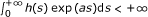 ;
; -
(v)
there exists γ > 0 such that
 and
and  .
.

 ;
; and
and  .
.Then zero solution of (1) is mean square exponentially asymptotically stable.
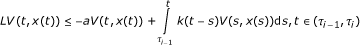
Proof. From (ii), we have

where D+ denotes the right Dini derivative. By Lemma 2.4,

for all t ∈ [τ i -1, τ i ). Now let's prove that

holds for all t∈ [τi -1, τ
i
) by mathematical induction for i = 1, 2,.... We stipulate  and
and  as i = 1 here and in the sequel. (11) is true for i = 1 immediately from (10). Assume that (11) holds for any i ≥ 1, then for t = τi we get

From assumption (iii) Then by use of (10) for all t ∈ [τ i , τi+1) we get

Thus by mathematical induction (11) is true for i = 1, 2,....
By Lemma 2.2, it follows (11) that

Then the mean square exponential asymptotic stability of (1) inherits from that of solutions of (2) under assumptions (iv) and (v). The proof is complete.
Corollary 3.2. If there exist positive numbers c1, c2 and V ∈ C1,2(R+ × Rn, R+) satisfying (i)-(iii) and
(v) in Theorem 3.1 and
(H1)  exp (as)ds < ∞;
(H2) there exists 0 < ρ < 1 such that  .
.
Then zero solution of (1) is mean square exponentially asymptotically stable.
Proof. Since implies  , the result is proved by Theorem 3.1.
Theorem 3.3. If there exist positive numbers c1, c2 and V ∈ C1,2(R+ × Rn, R+) satisfying
-
(i)
c1 ||x||p ≤ V (t, x) ≤ c2 ||x||p;
-
(ii)
there exist continuous and integrable function k : R+ → R+ and positive constant a such that for any i = 1, 2,...

holds when E||x (τi-1)||2 < θ for some constant θ > 0;
-
(iii)
there exist positive constants ω i such that for any i = 1, 2,..., we have

-
(iv)
there exists 0 < ρ < 1 such that
 ;
; -
(v)
 ;
; -
(vi)
τi ≤ t0 + i for all i ∈ N.

Then zero solution of (1) is mean square exponentially asymptotically stable.
Proof. Assumption (ii) implies

From Lemma 2.4, let h(t) = 0, for all t ∈ [τi-1, τ i ) we get

By denoting  , it can be proved that when ||x0||2 < δ0,

Holds for all i = 1,2,..., and

holds for all t ∈ [τ i-1 , τ i ) by mathematical induction. From (12), it is obviously true for i = 1. Assume that (14) is true for any i ≥ 1, then for all t ∈ [τ i-1 , τ i )), it is true that

and

From assumption (iii), we have that

Then by (ii),

for  . Then by mathematical induction (14) is true for i = 1,2,....
Combining z(t) ≤ 1, (iv) (vi) and the above results,

since τi-1≤ t ≤ τ i ≤ t0 + i.
Therefore  holds. The proof is complete.
Remark 1. Theorem 3.3 is not a simple corollary of Theorem 3.1, since the conditions (ii) and (v) in Theorem 3.3 is weaker than that in Theorem 3.1.
Remark 2. Theorem 3.3 shows that is not necessary condition for exponential asymptotical stability, which can also be found in Theorem 3.5.
3.2 Mean square non-exponential asymptotic stability
To show that the solution of (1) is mean square non-exponentially asymptotically stable, we have to prove that  and
and  . Now we prove the solution convergent to zero firstly.
Theorem 3.4. If there exist positive numbers c1, c2 and V ∈ C1,2(R+ × Rn, R+) satisfying
-
(i)
c1 ||x||p ≤ V (t, x) ≤ c2 ||x||p;
-
(ii)
there exist two continuous and integrable functions k, h : R+ → R+ such that for any i = 1, 2, ······
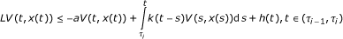

holds for some constant a > 0;
-
(iii)
there exist constants ω i such that for any i = 1, 2,······, we have

-
(iv)
there exists 0 < ρ < 1 such that
; -
(v)
.

Then zero solution of (1) is mean square asymptotically stable.
Proof. From (11), by Lemma 2.2 and by Lemma 2.3,

for t ∈ [τi-1, τ
i
). Noticing 0 < ρ < 1, for any ε > 0, there is k0 > 0 such that  where
where  . For h(t) is integrable, for any ε defined above, there is
  such that
  for
for  . It follows that

for  . By choosing
  , it follows (15) directly that for any ε > 0, we have
  for
for  when
when  . The proof is complete.
Theorem 3.5. If there exist positive numbers c1, c2 and V ∈ C1,2(R+ × Rn, R+) satisfying (i)-(v) in theorem 3.3 and
(H1) there exist continuous and integrable function
 satisfying
 and constant
 satisfying
 such that

for any i = 1, 2,...;
(H2) there exist constants  such that for any i = 1, 2,..., we have

(H3)  satisfies
  and
and  ;
;
(H4) there is constant 1 > d > 0 such that  ;
;
(H5) log (τ i - t0) ≥ i for all i = 1, 2,....
Then zero solution of (1) is mean square non-exponentially asymptotically stable.
Proof. By use of Theorem 3.3, we obtain

From (H 1), we have that

for all t ∈ [τi-1, τ i ). Consequently, we get

for all t ∈ [τi-1, τ i ) for i = 1, 2,... by mathematical induction from (H1)-(H2). From assumption

Since  satisfies and , then

By L'Hospital rule

From (H5) and d < 1,

Thus, combine (16) and (17) to show

Since holds under assumptions (i)-(v) in Theorem 3.3, we get

Therefore

The proof is complete.
Remark 3. Assumption (H5) in Theorem 3.5 can be replaced by  .
.
4 Example
Example 1. Consider a nonlinear impulsive stochastic Volterra equation of the form

for t ∈ (τ
k
, τ
k
+ 1) with  , where τ
k
= 2kand the impulse is defined as
, where τ
k
= 2kand the impulse is defined as

for all k ∈ N. λ1(k) and λ2(k) are random variables on  . Then the zero solution of (18) and (19) is mean square non-exponentially asymptotically stable.
Proof. By putting  , we have that

It follows that

Since

we have

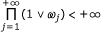
for all j > 0. In addition,

and

hold. By Theorem 3.4, it is true that

Next, we prove

From (20),

Since  and log τ
k
= k, we finish the proof by Theorem 3.5.
and log τ
k
= k, we finish the proof by Theorem 3.5.
References
Taniguchi T: The exponential stability for stochastic delay partial differential equations. J Math Anal Appl 2007, 331: 191–205. 10.1016/j.jmaa.2006.08.055
Wan L, Duan J: Exponential stability of non-autonomous stochastic partial differential equations with finite memory. Stat Probab Lett 2008, 78: 490–498. 10.1016/j.spl.2007.08.003
Luo J: Fixed points and exponential stability of mild solutions of stochastic partial differential equations with delays. J Math Anal Appl 2008, 342: 753–760. 10.1016/j.jmaa.2007.11.019
Sakthivel R, Luo J: Asymptotic stability of nonlinear impulsive stochastic differential equations. Stat Probab Lett 2009, 79: 1219–1223. 10.1016/j.spl.2009.01.011
Sakthivel R, Luo J: Asymptotic stability of impulsive stochastic partial differential equations with infinite delays. J Math Anal Appl 2009, 356: 1–6. 10.1016/j.jmaa.2009.02.002
Brauer F: Asymptotic stability of a class of integro-differential equations. J Diff Equ 1978, 28: 180–188. 10.1016/0022-0396(78)90065-7
Burton TA, Mahfoud WE: Stability criterion for Volterra equations. Trans Am Math Soc 1983, 279: 143–174. 10.1090/S0002-9947-1983-0704607-8
Kordonis IGE, Philos ChG: The behavior of solutions of linear integro-differential equations with unbounded delay. Comput Math Appl 1999, 38: 45–50. 10.1016/S0898-1221(99)00181-9
Murakami S: Exponential asymptotic stability for scalar linear Volterra equations. Diff Integral Equ 1991,4(2):519–525.
Appleby JAD, Reynolds DW: On necessary and sufficient conditions for exponential stability in linear Volterra integro-differential equations. J Integral Equ Appl 2004,16(3):221–240. 10.1216/jiea/1181075283
Appleby JAD, Reynolds DW: Subexponential solutions of linear integro-differential equations and transient renewal equations. Proc R Soc Edinb 2002, 132A: 521–543.
Appleby JAD, Reynolds DW: On the non-exponential convergence of asymptotically stable solutions of linear scalar Volterra integro-differential equations. J Integral Equ Appl 2002,14(2):109–118. 10.1216/jiea/1031328362
Mao X, Riedle M: Mean square stability of stochastic Volterra integro-differential equations. Syst Control Lett 2006, 55: 459–465. 10.1016/j.sysconle.2005.09.009
Appleby JAD, Reynolds DW: Non-exponential stability of scalar stochastic Volterra equations. Statist Probab Lett 2003,62(4):335–343. 10.1016/S0167-7152(03)00035-X
Appleby JAD, Riedle M: Almost sure asymptotic stability of stochastic Volterra integro-differential equations with fading perturbations. Stoch Anal Appl 2006,24(4):813–826. 10.1080/07362990600753536
Appleby JAD: Subexponential solutions of scalar linear Ito-Volterra equations with damped stochastic perturbations. Funct Differ Equ 2004,11(1–2):5–10.
Appleby JAD: Almost sure subexponential decay rates of scalar Ito-Volterra equations. Electron J Qual Theory Differ Equ., Proc 7th Coll QTDE, Paper no 1 2004, 1–32.
Appleby JAD, Freeman A: Exponential asymptotic stability of linear Ito-Volterra equations with damped stochastic perturbations. Electron J Probab 2003,8(22):22.
Appleby JAD, Reynolds DW: Decay rates of solutions of linear stochastic Volterra equations. Electron J Probab 2008,13(30):922–943.
Becker LC: Function bounds for solutions of Volterra equations and exponential asymptotic stability. Nonlinear Anal 2007, 67: 382–397. 10.1016/j.na.2006.05.016
Acknowledgements
The authors sincerely thank the anonymous reviewer for his careful reading, constructive comments and fruitful suggestions to improve the quality of the manuscript. This article is partially supported by NSFC (No. 11001173).
Author information
Authors and Affiliations
Corresponding author
Additional information
Competing interests
The authors declare that they have no competing interests.
Authors' contributions
DZ and DH conceived of the study. DZ carried out most of the analysis and drafted the manuscript. DH revised and commented on the draft. All authors read and approved the final manuscript.
Rights and permissions
Open Access This article is distributed under the terms of the Creative Commons Attribution 2.0 International License (https://creativecommons.org/licenses/by/2.0), which permits unrestricted use, distribution, and reproduction in any medium, provided the original work is properly cited.
About this article
Cite this article
Zhao, D., Han, D. Mean square exponential and non-exponential asymptotic stability of impulsive stochastic Volterra equations. J Inequal Appl 2011, 9 (2011). https://doi.org/10.1186/1029-242X-2011-9
Received:
Accepted:
Published:
DOI: https://doi.org/10.1186/1029-242X-2011-9