
Abstract
Mobile crowd computing (MCC) has emerged as an ideal platform for accessing required computing services from public-owned mobile devices in the vicinity, not requiring to going to the Cloud. But it may happen that the service is not available within the network (of the consumer) always. In this case, a carrier is needed, which carries the request to the service provider (in another network), gets the service from it and handovers to the consumer. But the mobility of the service consumer, provider, and the carrier poses a great challenge in binding between them for service request and service exchange. Device mobility is considered as one of the performance metrics in MCC. Though it is not trivial to measure, the efficacy of MCC heavily depends on this metric. To mitigate this issue, in this paper, we propose a service provisioning model in MCC based on the mobility patterns of the above-mentioned three entities. We applied a mobility prediction algorithm on the UCSD dataset that comprises real-traces of 235 mobile device users for 78 days across 402 access points (APs). In this experiment, we focussed mainly to get the information: (a) average time gap after a user connects to an AP, (b) average duration he/she remains connected to an AP, and (c) a set of users who remains connected to a particular AP simultaneously. Knowing the mobility patterns of the service consumer, provider, and the carrier, in terms of the above-mentioned information, is helpful to bind them in particular time frames. This allows avoiding the liveness problem (consumer waits for the service indefinitely) and availability problem (carrier returns with the service but cannot find the consumer).
1 Introduction
1.1 Mobile crowd computing
The deep penetration of cellular networks and the low-cost and affordability of the mobile devices have increased their popularity and usage on a massive scale. It is estimated that by 2020, the shipment of smartphones (not including tabs) will reach 6 billion globally [1, 2]. Thanks to the ever-increasing capacity (hardware and software) of the smart mobile devices (SMDs) like smartphones and tabs along with increasing battery capacity and efficient energy management [3], they are increasingly being used as the primary computing device by many people. Due to the flexibility and mobility, these powerful SMDs can be a great prospect for offering computing services anywhere. Establishing an ad-hoc computing facility using the public-owned (crowd’s) SMDs is known as mobile crowd computing (MCC) [4]. The widespread highspeed cellular networks and abundantly available internet APs have fuelled the feasibility of such systems where the SMDs can exchange computing services with peer SMDs straightforwardly. The MCC not only provides a cheap and flexible computing facility, but it also offers an energy-efficient and sustainable computing infrastructure [5, 6].
1.2 Mobile crowd computing vs mobile cloud computing
Though these two terms seem nearly homophones, they are different altogether. Mobile crowd computing refers to an ad-hoc computing setup utilising the public mobile devices [7] whereas mobile cloud computing typically refers to offloading heavy applications or tasks from mobile devices to the cloud [8, 9].
1.3 Asymmetrical competences of SMDs
As the SMDs have been integrated with our daily life, consumers are asking for more and more effective and functional services to satisfy their needs using their SMDs. This has led to the continuous development of sophisticated mobile applications (apps) that are supposed to make our lifestyle easier. To run most of these apps, certain hardware and software resources are required. But all the SMDs do not boast equal capacity or functionality. Some of them are high-end with greater capacity and can afford to host various types of apps, while some might have inferior configuration and capacity; hence, they may not afford to have/run the resource-demanding apps.
1.4 Proposed service provisioning scheme in MCC
Now, let us theorise an MCC environment where a low-end SMD can get/hire the service, that it requires but does not have, from one SMD that has the concerned service. To make it simple, software and hardware capabilities can be delivered and consumed as services, and if an SMD (or its user) needs such service, it may contact one nearby SMD which has the service and is willing to give/lend that. If the service seeker (SS) is not in a direct contact of the service provider (SP) (they are in different networks) then one mediator/agent, we call it a service carrier (SC), may be employed which carries the service request to the SP, gets the service from it and handovers to SS. The SMD may provide the service on profit (gets something in return) or non-profit (doing social service) basis. Since this approach involves latency, it particularly suits the delay-tolerant applications (DTA), which may afford to wait for the required service.
1.5 Service lending scenarios in MCC
The proposed service lending scheme in MCC can be used in several real-life scenarios and has a wide range of significant applications. MCC will play a critical role for anytime-anywhere computing service provisioning through impromptu collaboration. These services may include educational programs, multimedia services, business applications, instant messaging, etc. MCC may also be useful for hiring network services such as routing and packet forwarding to other nodes. Moreover, ad-hoc environments such as military battlefields and disaster management areas also can make use of MCC.
Consider the following real application scenarios of MCC to visualise the advantage of MCC better:
-
Scenario 1 John, while sitting in the student canteen, downloads a research article that seems to be related to his project. But after downloading, he finds that the document is not opening on his SMD as it is in some unknown format. John has a pdf reader application installed in his device, and if the document could be converted to pdf, he could read it. But he does not have any such conversion app. So, he searches the network for a buddy, having the conversion service. And thank goodness, he found one such and got the file converted to pdf. John is elated and dives into the paper without delay.
-
Scenario 2 Lilly goes to a shopping mall to buy a laptop. The salesman shows her a couple of models from different companies. Though the salesman tries his best to explain to her about the features of the products, Lilly wants to be sure about the advantages and disadvantages, in a comparative manner, of the products the salesman showed her. Her smartphone is not able to help her because she does not have any such benchmarking applications installed. She also tries to visit the websites of the companies of the products using her smartphone, but due to the inferior cellular connection, she cannot manage to open all the websites either. In an MCC environment, she requests for a benchmarking service to an SP, in her vicinity. The SP agrees to help her and makes the comparison for her and sends her the comparison result. Satisfied with the best one (according to her requirements) she bought the laptop and went home happily.
-
Scenario 3 Merry intends to fill up the library subscription form while sitting in the college library. But the form is in pdf format, and she does not have the edit option in her pdf reader version (the pdf reader might be a pirated one or with a limited licence). So, she tries to convert it into a Word document. But again, she does not have the conversion software. So, she searches for an SP which can provide this conversion service within the network. Unfortunately, there was no SP available in the network. So, an SC comes to her rescue, which goes out and searches for the required service in other networks. Once it finds the service, gets from that SP, returns to the previous network, and delivers the converted Word document to Merry. But, interestingly, Merry is not aware of all these processes. The MCC system took care of all these, transparently.
1.6 Issues in service provisioning in MCC
Among others, the major challenge in MCC is handling the issues caused by the random mobility of the participating SMDs which can join and leave the network any time. In the proposed model, what happens if the SC returns with the requested service and finds that the concerned SS is not present in the network at that time? Or what happens if the SS waits for indefinite time not knowing when the SC will return to the network with the service?
1.7 Suggestive solution
If the mobility patterns of the SMDs are studied, especially in a campus-based MCC environment, the in and out time of a particular SMD to a particular network can be predicted. And the SC and SP are selected according to the predicted contact time between SS, SC, and SP.
1.8 Contribution of this paper
The major highlights of this paper are as follows:
-
Lays out a service provisioning model in MCC.
-
Find out relative mobility and stability among the service requester, provider, and the carrier based on their individual mobility pattern.
-
Based on the mobility pattern, predict the contact times between these three entities. The mobility prediction is made using the mobility prediction algorithm described in [10].
-
The prediction is performed and tested on real data traces which are collected from a large number of mobile device users.
1.9 Organisation of the paper
The rest of the paper is organised as follows. Section 2 mentions some related works and patents. The system architecture is presented in Sect. 3. Section 4 provides the details of the experiment, including the results and validation. The paper is concluded in Sect. 5.
2 Related works
Since the concept of MCC is relatively new, we couldn’t find research works that exactly matches that of the proposed in this paper. Below we list some prominent works related to the core concepts that are essential in realising MCC.
2.1 Mobility tracking
Several approaches are proposed to predict the mobility of a node. Most of them use certain methods like GPS (global positioning system), RSS (received signal strength), etc. which have several limitations, as mentioned in [11], and listed in Table 1. Researchers tried different means to track human mobility by analysing their accompanying devices. For example, to analyse human mobility, Smoreda et al. [12] discussed the data collection methods from mobile phones. In [13], users’ mobility is analysed and characterised with the data collected from smartphones and smartwatches. Williams et al. [14] measured human mobility based on the user’s mobile phone records and GIS data. Wang and Ak yildiz [15] predicted user mobility with respect to a set of mobile switching cells, based on the aggregated history of the mobile users and system parameters. To determine the user’s current location, Ma et al. [16] considered the user’s movement and the current system time.
2.2 Mobility-aware service discovery and delivery
Deng et al. [17] proposed a mobile service provisioning architecture for sharing services among the mobile device user community. Tyagi, Som and Rana [18] proposed a reliability-aware data delivery protocol for MANET (mobile ad-hoc network) based on AODV (ad-hoc on-demand distance vector), considering the speed of intermediate nodes in the route. Vadde and Syrotiuk [19] studied the impact of various factors such as QoS architecture, routing protocol, medium access control protocol, offered load, and mobility and their interactions on service delivery, based on different measures like real-time throughput, total throughput, and average delay. Various service discovery protocols are discussed in [20] while a decentralized service discovery mechanism is presented in [21].
2.3 Leader selection in mobile and wireless network
Several leader election algorithms and approaches are proposed for wireless networks [22,23,24,25], Similarly, several works available on leader selection in MANETs [26,27,28,29,30,31].
3 System architecture
3.1 The service provisioning model in MCC
High mobility and heterogeneous resources of the SMDs in an MCC environment has posed a challenge in deciding the right architecture for it. The three traditional architectures, namely, centralised, P2P, and hybrid, can be applied to MCC as well.
The centralised model, where a centralised node is responsible for coordinating the service provisioning, is suitable for small-scale MCC. The main drawback of this model is that it is prone to congestion, single-point failure, and DoS (denial of service) attack.
The P2P model does not justify the notion of MCC presented in this paper. In this architecture, in the absence of a centralised coordinator, each SMD has to maintain the information of all other SMDs in the whole network. But the point is that if an SMD has the resources to keep track of all other SMDs’ various information, then it can be assumed that they are rich enough for not requiring to solicit services from someone else.
The hybrid model seems to be the most suitable for the concept of MCC in the context of this paper. In this model, all the APs are considered as different disjoint clusters. Within a cluster, one leader is selected or elected. All SMDs within the cluster forward the service request to the leader. If the requested service is not available in the cluster, then searching will be done in another cluster, typically in the clusters that are very close to the original cluster such as the siblings, parent, or immediate child.
If all the clusters are dense in nature, i.e. all the clusters are placed near to each other, then it is easy to find the service across the clusters; but if the clusters are sparse and placed far from each other and also not directly connected, as shown in Fig. 1, then the mobility property plays a crucial role in searching as well as getting the service. In such cases, an SMD is selected, within the cluster, that has the highest mobility in the requesting cluster. It goes to another cluster that might have the requested service, collect the service, and get back to the requesting cluster and provide to the requesting node.

Clustering in a dense network and b sparse network
3.2 Key components
Before diving into the details, let us be familiar with the key components of the proposed system. Some of the crucial terms we encounter throughout the article are as follows:
Service Seeker (SS) An SMD (or SMD user) which needs a service that it does not have.
Service Provider (SP) An SMD which has the service that is requested by a SS and it (or the mobile phone user) is willing to lend/provide the service.
Service Carrier (SC) An SMD which, if required, carries the request (with necessary details) of an SS to an SP and gets back the result/service to the SS.
Access Point (AP) Usually, a Wi-Fi router to which the SMDs are connected. Also, each AP forms an individual cluster comprising the SMDs connected to it. The APs are not connected to each other.
Reference Node (RN) It is one of the most resourceful and highly stable SMDs in the cluster. It acts as the leader of the concerned cluster and is responsible for keeping the information of all the peers within the cluster so that when it receives a service request form an SS, it can rightly suggest the most suitable SP or SC to the SS, regarding services that could be provided by the SMDs in the network. Under each AP, at any point of time, an RN should be present.
3.3 Working of the proposed system
The working of the proposed system is stepwise described in the following:
-
1.
As mentioned earlier, under each AP, an RN is maintained, which holds the information of all the peer SMDs in the same network.
-
2.
When needed, an SMD refers to the concerned RN for probable SP.
-
3.
If the requested service is available within the own network (AP) then:
-
(a)
RN suggests SS the most suitable SP.
-
(b)
SS requests the SP for the service.
-
(c)
SP provides the service to the SS.
This scenario is depicted in Fig. 2.
-
(a)
-
4.
If the service is not available in the network, the RN suggests a suitable SC under it that has a higher probability of moving to another network where the service may be available and come back soon. If the SC is willing to do this job then:
-
(a)
The SC takes along the request with the required data/inputs to another network and requests the RN of that network (remote RN) to suggest the most suitable SP (remote SP) for the job.
-
(b)
As per the suggestion from the remote RN, the SC requests the suggested SP for the desired service.
-
(c)
SC gets the service, returns to the previous AP (home network), and hands over the service to the SS.
This scenario is depicted in Fig. 3.
-
(a)
-
5.
If the service is not found in the other network also, any one of the following measures can be adopted:
-
(a)
The searching cycle might go on in other networks.
-
(b)
SS can try later to get the service.
-
(c)
The request is aborted.
-
(a)
The workflow of the whole system is presented in Fig. 4.

Service is available within the network

Service is not available within the network

The workflow of the proposed service provisioning system
3.4 Issues in the proposed system
Some of the following mentioned issues are crucial and need to be addressed for successful implementation of the proposed system for service provisioning:
-
Synchronisation between SS and SC Since the nodes in an MCC are typically dynamic in nature, it is crucial to synchronise the presence of SS and SC in the same network. The absence of which may result in the following significant problems (see Fig. 5):
Fig. 5 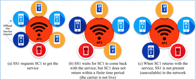
Availability and Liveness problems
-
Liveness problem The SS assigns the job of getting the service from a different network to SC (Fig. 5a). But SC may not come back with the service to the SS network, as illustrated in Fig. 5b. It is treated as liveness problem. The liveness problem can be avoided if an SMD is selected as SC that has high mobility.
-
Availability problem On the contrary, it may happen that the SC returns with the service but finds that SS is not present in the network, as illustrated in Fig. 5c. To avoid this availability problem, we require a mechanism that makes synchronization between the SS and SC and so that SS remains in the network when SC comes back with the service.
-
-
Selecting a node with high mobility We just mentioned that a highly mobile SC could help in avoiding the liveness problem. Also, an SC with high mobility has a better chance to get a service in different networks at different times. Because, if the service is not available in one network, a highly mobile SMD can move to other networks and find the service. That implies, the search for service is widely propagated across several networks. But identifying the node that is highly mobile is not straight forward. Several approaches are proposed in this regard, as discussed in Sect. 2.
-
Calculating the probability and the probable time of meeting SS with SC again In addition to being highly mobile, an SC should be selected based on the contact frequency with the SS. This requires calculating the number of times the SC comes in contact with the SS.
-
Calculating the overall contact period of SC with the SP It is very crucial to know the approximate time for which the SP will remain in contact with the SC because if the stay-time of the SP in the network (while providing the service) is less than the amount of time required for serving the request, the purpose is not fulfilled. So, the contact period between SP and SC should be larger than that of service providing time.
-
Deciding on the optimal waiting time of SS for SC to bring the service The SS cannot wait indefinitely for the SC to get the service for it. This might result in an indefinite lock in for a certain service. So, there should be a timeout value for SS as well as SC to wait or search for the particular service.
-
Permissible time an SC can spend in other networks while carrying a pending service request When carrying a service request form an SS an SC cannot stay in other networks for a very long or very small duration. If SC stays for an abnormally long time outside of the network, the SS may starve for the service, and if the SC stays in the external network (from it is supposed to get the service) for a very small duration, it may not get enough time to receive the service. Therefore, finding out the optimum time duration an SC can stay in another network is very important.
-
Weighing the reliability of SC How to be sure that the designated SC will surely get the service? Due to several reasons (intentional or circumstantial, SC may not deliver the service to the SS, even after agreeing to do that. Though exact assessing is not trivial, an approximation should be made on the reliability of SC in getting the service assuredly. To tackle this problem, the SC can be incentivised so that they will find interest in delivering the service to SS successfully.

3.5 Essential criteria of the key components
From the above discussions, now we are able to get a clear depiction of the desirable properties of the key components mentioned in Sect. 3.2.
SS Ideally, should be stable in the network, so that whenever SC returns to the network, it should be available to receive the service.
SC Since SC plays a crucial role in getting the requested service while selecting an SMD as an SC, the following crucial factors should be considered:
-
A node with high mobility should be chosen as an SC since the highly mobile node has a high frequency of changing its position and comes in contact with different networks and thus, having a high probability that it will search the service providing node faster.
-
In spite of the high mobility, the SC should regularly be in contact with the SS for service delivery.
-
The SC should be present in the network of the SP for sufficient duration so that it can receive the service fully and successfully.
-
The SC should have sufficient memory to carry the service request and the service itself.
SP Ideally should be stable in the network. If not, then, it should be stable at least for the contact period with SC so that the service can be provided completely to SC.
RN The RN is also an important entity which should have the following characteristics:
-
Ideally, should be very much stable in the network.
-
It should be active enough to retrieve the information of the SMDs whenever they enter the network.
-
To store the information of all other SMDs, the RN must have sufficient hardware and software resources.
-
It should have adequate decision-making capability for suggesting SP and SC.
4 Materials and methods
4.1 UCSD dataset
To implement our system for finding relative mobility, we used the UCSD trace dataset,Footnote 1 obtained from the University of California, San Diego (UCSD). Marvin McNett and Geoffrey M. Voelker of the University of California, San Diego conducted a study of the movements of as many as 275 students of the university for the period from 22nd September 2002 to 8th December 2002—a total of 78 days [37]. The trace data was collected for 402 APs within a range of approximately 130 m × 130 m square area. In the trace collection, the users were given a Jornada personal digital assistant (PDA) which recorded the trace information with the help of a data collection tool called Wireless Topology Discovery (WTD), an in-house developed software. The WTD software sampled and collected the trace data before uploading them periodically to a server. The users are identified through the Media Access Control (MAC) addresses of their devices’ wireless network cards. It is assumed that there is a one-to-one mapping between users and wireless network cards. However, the mapping is anonymous, i.e. there is no mapping between usernames and MAC addresses.
After a user’s device was powered on, the WTD software collected the following data periodically during the 11-week trace period:
-
The signal strength of each detected AP.
-
MAC address of each AP that was detected.
-
Current AP association.
-
The version number of the WTD program.
-
Type of device (Jornada 548 or 568).
-
Power state the device is running on (connected to an AC socket or using battery power).
It is to be noted that the WTD program recorded the MAC address of all APs that were detected by the PDA, not only the AP the PDA was associated with at the time of sampling. This is evident from the recorded data contained in the trace file wtd.csv (described later in this section). A sampling of data was done with a time interval of 20 s, i.e. the WTD software recorded data after every 20 s. During data collection, when the local data file reached a critical size, the WTD software contacted the data collecting server and uploaded the file at the next opportunity. A feature of the WTD software was that it automatically checks the server for new updates and downloads and installs them, so that it may adapt to unexpected problems if necessary.
Key terms The key terms used in the trace data analysis are as follows:
-
User A user is someone who has a mobile device connected to one of the AP in the context.
-
AP session An AP session is a contiguous time period for which a user’s device was associated with a particular AP in the UCSD campus.
-
User session A user session is a contiguous time period in which a user’s device is powered on and is able to detect the signals of nearby APs. A user session includes the user’s movements among different APs.
Contents The dataset contains three files, namely, ap_locations.csv, README, and wtd.csv. The files ap_locations.csv and wtd.csv are trace files containing the data recorded by the UCSD researchers and README, a text file, is the metadata file of these two trace files.
The file ap_locations.csv is a file of comma-separated values comprising 4 fields as follows:
-
AP_ID: Unique identifier assigned to the AP.
-
X_COORDINATE: X-coordinate (in feet) of AP w.r.t. campus coordinate system.
-
Y_COORDINATE: Y-coordinate (in feet) of AP w.r.t. campus coordinate system.
-
Z_COORDINATE: Z-coordinate (in feet) of AP w.r.t. campus coordinate system.
The file wtd.csv is a file of comma-separated values comprising 7 fields as follows:
-
USER_ID: Unique identifier assigned to the user.
-
SAMPLE_DATE: The date the sample was taken by the WTD software.
-
SAMPLE_TIME: The time the sample was taken by the WTD software.
-
AP_ID: Unique identifier assigned to the detected AP.
-
SIG_STRENGTH: Strength of AP signals received by the device.
-
AC_POWER: Whether the device used AC power (1) or battery (0).
-
ASSOCIATED: Whether the device is connected to the AP (1) or it is in the range but not connected (0).
It is to be noted that the trace file wtd.csv and the metadata file README, both do not mention the field SAMPLE_DATE, probably due to the human error or as per the researchers’ discretion. A snapshot of the 3D view of APs are shown in Fig. 6, and the snapshots of the files ap_locations.csv and wtd.csv are shown in Figs. 7 and 8, respectively.

Snapshot of the 3D view of APs

Snapshot of the file ap_locations.csv

Snapshot of the file wtd.csv
4.2 Our work with the dataset
In this section, we outline what has been done on the dataset and why.
4.2.1 Summary of the work performed
We performed the following operations on the original wtd.csv file in steps to obtain information:
-
1.
Eliminate all the users with associated value ‘0’ and create a separate file which includes all the users with associated value ‘1’.
-
2.
Find out the average time gap (in seconds) after which a user comes back and reconnects to the AP, he/she was connected to earlier. We calculate separate average time connection per AP for every user in the network and name these files on the name of users, for example, the file of user with ID ‘1’ is saved as 1.avg.txt.
-
3.
Find out at least four users who are connected to a particular AP at the same time. For example, four users—user ‘32’, user ‘54’, user ‘97’ and user ‘21’ are connected to AP ‘245’ at time 13:12:54, 13:12:57, 13:12:46, and 13:13:00 respectively. Here, the maximum time difference is 14 s, which is not much, hence ignored; i.e., we consider that they are connected at the same time frame.
-
4.
To find such combinations, we write a program in Python and identify a set of four users who are connected at the same time with a particular AP.
-
5.
Calculate average connection time (ACT) (the average time a user is connected to a particular AP) of the users.
4.2.2 Expected output
After performing the above-mentioned operations, we get the followings:
-
(a)
Average time (in seconds) after which a user connects to an AP.
-
(b)
Average duration (in seconds) a user remains connected to an AP.
-
(c)
A set of 4 users who are simultaneously connected a particular AP.
The first (a) and second (b) types of information are useful to find out the movement of the users that at which time the user will come again in contact with the AP and how much time a user spends. And the third information will help to find the expected future location (AP) of a group of users, i.e. when they will be in contact with that particular AP.
4.3 Details of operations performed to process the UCSD trace file
In this section, we discuss, in detail, the operations that we performed on the UCSD trace file wtd.csv for extracting the information that we required to implement our proposed architecture.
4.3.1 Remove noise
First, we filter according to the ASSOCIATED value available from the downloaded wtd.csv file. This value is used to calculate/identify the neighbours of a node (user). To make it clear, suppose three nodes at a time are in the range of an AP but the first node is only connected to this AP and the second and the third nodes are not connected or connected to some other AP. Then, they can be treated as neighbours of each other. To eliminate entries with ASSOCIATED value ‘0’ (i.e., not connected), we write a program in Java which use MySQL in the backend to access the file. Snapshot of the output is shown in Fig. 9.

Snapshot of the dataset after eliminating not connected entities
4.3.2 Calculate the time gap after a user returns to the network again
After doing away with the unwanted values (nodes that are not connected), we aim to estimate the average time period after which a user comes back to the contact (ASSOCIATED) with the particular AP. A Python program is written for this, which considers the details of the connected nodes (users) during the data tracing period, i.e. for 78 days. Figure 10 gives an idea of the average time after which a user gets connected to a particular AP.

Snapshot of ACT of all the users to a particular AP
This is important to get rid of the availability problem. Based on this information, the SMD that is highly mobile and has a high possibility of meeting with the SS after getting the service from the SP is selected as SC.
4.3.3 Identifying a group of SMDs connected to an AP simultaneously
To continue our experiment, we create a find group of 4 users who are connected to an AP at the same time. An instance of such set is shown in Table 2. It can be observed that a group of 4 users are connected to AP ‘354’ on 24-sept between 13:00:51 to 13:01:08. In this table, there are 6 columns as follows:
-
USER_ID indicates a device unique ID which is carrying by the user.
-
SAMPLE_DATE shows the time at which the record is taken.
-
SAMPLE_TIME shows the time of connection.
-
AP_ID indicates connected AP with the user.
-
ASSOCIATED, as mentioned earlier, denotes the active connection.
-
AVERAGE is the ACT after which a user is connected to that AP.
4.3.4 Selecting the reference node
From Table 2, we select an SMD as an RN. To find the RN, we calculated the ACT of the SMDs, which indicate how long an SMD is available in the network and how many occasions and for how long they are disconnected. This is important for a node to active in the network to provide or access services.
We divide a day into 12 sessions of 2 h each and track the movement of the SMDs for each session. For example, the first session of 2 h’ starts from 00:00:00 to 02:00:00, and we calculate ACT of User 42, User 208, User 232, and User 242 in this time interval. Similarly, the ACTs of these users are collected for all sessions, as shown in Table 3. Using these ACT, we calculate average time and standard deviation.
To calculate the mean of ACT, collected for different sessions, we use Eq. 1.
Where, µ ⇒ Mean, s ⇒ No. of sessions, xi ⇒ Values, N ⇒ Total no. of values.
For calculating the standard deviation, we use Eq. 2.
Where, σ ⇒ Standard deviation, N ⇒ Total no. of values, xi ⇒ Values, µ ⇒ Mean of N values.
Using the mean value and the standard deviation, we spot the user (SMD) that stays in the network for most of the time. Within the considered 4 users, we find out that User 41 is more frequently available in the network. For comparative demonstration, ACT graphs of User 41 and User 208 are shown in Fig. 11.

Average connection time graph of a User 41 and b User 208
From Fig. 11a, it can be observed that the ACT of User 41 is close to its mean and standard deviation, which shows that there is less variation in the ACT. Whereas, in Fig. 11b, we can see that there is a large difference between standard deviation and ACT of User 208, and the variation of ACT is more than User 41. So, we consider User 41 as a better choice to be an RN.
4.3.5 Assessing the relative stability
Another decisive criterion for choosing an SMD as an RN is relative stability (RS). To calculate the RS of each user, we use the algorithm proposed in [7], as shown in Eq. 3. The RSs of the four users in consideration are shown in Table 4.
where \(s_{t}^{x}\) ⇒ Relative stability, \(m_{t}^{x}\) ⇒ Current neighbour list and is defined by Eq. 4.
The RS graphs for User 41, User 208, User 232, and User 242, obtained from Table 4, are shown in Fig. 12.

Relative stability graph of a User 41 b User 208 c User 232 d User 242
From Fig. 12a, it can be observed that the RS for User 41 is varying very close to the standard deviation and mean, which are almost equal. In the case of User 208 also, the RS is varying around standard deviation, as can be seen in Fig. 12b. But the difference between mean and standard deviation is much higher for User 232, and this user is not active/relatively stable for most of the time, as can be seen in Fig. 12c, hence, not suitable as the RN. User 242 is not active at this duration (Fig. 12d). So, comparing these 4 graphs, we found that User 41 and User 208 are the two choices to be selected as the RN. But the ACT of User 41 is better than User 208; therefore, we select User 41 as the RN.
4.3.6 Calculate the latency of the users in returning to the AP
Now, we estimate when a user returns to the previous AP after it left. It is important because if a SS leave the AP, it should come back as soon as the service is available which is brought by an SC. Similarly, for an SC also, it is crucial to return with the service as soon as possible. To calculate the return time, we use the ACT of the users. For this calculation, we use Table 5, which includes all the values required to calculate. An instance of the four considered users is shown in the table. It can be seen that the SCs (User 208 and User 242) returns to the network after 0.085 days.
Figure 13 shows the arrival time of the four users when they return after leaving the A; in this case, AP 354. User 41 and User 232 are SSs, which require services and User 208 and User 242 are SCs, which are mobile in nature and supposed to bring service to the requesting node.

Predicted arrival time of a User 41 b User 208 c User 232 d User 242
The estimated time of returning of User 208 and User 242 to the AP is at 13:30:00, as shown in Table 5. It is assumed that they bring the service along with them. Hence, at that time, the SSs, i.e. User 41 and User 232, should be present in the network to receive the requested services.
The standard deviation is used to measure variation between the ACT of the sessions. From Fig. 13, it is evident that though the users seem to be roaming around the campus across the sessions, they all are connected to the particular AP (354) between session 6 and 7, which indicates time duration 12:00:00 to 14:00:00, and this is in range of our predicted time (13:30:00).
4.3.7 Validating the proposed mobility estimation scheme
Now let us check how our proposed approach for estimating the relative mobility works in a different scenario. Let us consider that User 41 and User 208 are the SSs (which request for services that are not available in the network) and User 232 and User 242 are the SCs. The estimated time of returning of User 232 and User 242 to the AP is at 16:00:00 on 25-Sept, as shown in Table 6.
Now, let us check if the SCs can deliver the service to the SSs at the time of contact. As we have seen, according to our estimation, the predicted time of contact is 25-Sept at 16:00:00 pm (approx.), which belongs to session 8 (14:00:00–16:00:00). From Fig. 14, we can see that at that time, User 208 and User 41 are not active; and User 242 is not active on 25 Sept, whereas User 232 is active on that session but connected to some other AP which are not in the range of the SS. So, SSs are not able to get the requested service from the SCs on the predicted time.

Nodes did not arrive on the predicted time
In the first case (Fig. 13), users arrived at the predicted location on time, but in the second case (Fig. 14), the same does not happen. So, using these two scenarios, we can conclude that to predict the future time on which SS and SC may communicate, a fixed pattern is required.
5 Conclusions and future scope
Though mobile crowd computing is a brilliant opportunity for sharing computing services in a flexible and ad-hoc manner, the failure in addressing the mobility factor of the participating mobile devices will lead to an unsuccessful implementation. The mismatch in the contact time between the service consumer, provider, and the carrier (that acts as a mediator to exchange the service between the provider and the consumer) will prohibit in exchanging the service. Hence, it is very important to know when they will be in contact with each other so that the service can be exchanged. In a mobile setup, it is not trivial to know. But if the mobility patterns of the devices are tracked, the location of the devices and the duration for which they remain in a network can be predicted. In this paper, applying a mobility prediction algorithm on a dataset of real mobility traces, different mobility-related information are extracted. These information are utilised in selecting the service carrier and the provider so that the availability (consumer waits for the service indefinitely) and liveness (the carrier returns with the service but cannot find the consumer) problems can be averted. The shortcoming of this work is that the dataset that is used in the experiment is not wide enough; it is only of 78 days. And also, the traces do not follow a fixed pattern whereas our proposed model is based on a fixed mobility pattern because, in real life, most people do their task in a fixed pattern like they wake up in the morning, take breakfast, go to their work, stay at the workplace till evening, return back to their home and, generally, follow the same pattern, except holidays. So, experimenting with a dataset of fixed mobility patterns would have yielded a better prediction.
References
GSMA. Smartphones to account for two thirds of world’s mobile market by 2020 says new GSMA intelligence study. 11 September 2014. https://www.gsma.com/newsroom/press-release/smartphones-account-two-thirds-worlds-mobile-market-2020/. Accessed 17 Aug 2018
Statista. Global smartphone shipments forecast from 2010 to 2022 (in million units), May 2018. https://www.statista.com/statistics/263441/global-smartphone-shipments-forecast/. Accessed 17 Aug 2018
Pramanik PKD, Sinhababu N, Mukherjee B, Padmanaban S, Maity A, Upadhyaya BK, Holm-Nielsen JB, Choudhury P (2019) Power consumption analysis, measurement, management, and issues: a state-of-the-art review on smartphone battery and energy usage. IEEE Access 7(1):182113–182172
Pramanik PKD, Pal S, Pareek G, Dutta S, Choudhury P (2018) Crowd computing: the computing revolution. In: Lenart-Gansiniec R (ed) Crowdsourcing and knowledge management in contemporary business environments. IGI Global, Hershey, pp 166–198
Pramanik PKD, Pal S, Choudhury P (2019) Smartphone crowd computing: a rational solution towards minimising the environmental externalities of the growing computing demands. In: Das R, Banerjee M, De S (eds) Emerging trends in disruptive technology management. Chapman and Hall/CRC, New York, pp 45–80
Pramanik PKD, Pal S, Choudhury P (2019) Green and sustainable high-performance computing with smartphone crowd computing: benefits, enablers, and challenges. Scalable Comput Pract Exp 20(2):259–283
Pramanik PKD, Choudhury P, Saha A (2017) Economical supercomputing thru smartphone crowd computing: an assessment of opportunities, benefits, deterrents, and applications from India’s perspective. In: 4th International conference on advanced computing and communication systems (ICACCS-2017), Coimbatore, India
Noor TH, Zeadally S, Alfazi A, Sheng QZ (2018) Mobile cloud computing: challenges and future research directions. J Netw Comput Appl 115:70–85
Shiraz M, Sookhak M, Gani A, Shah SAA (2015) A study on the critical analysis of computational offloading frameworks for mobile cloud computing. J Netw Comput Appl 47:47–60
Choudhury P, Nandi S, Debnath NC (2012) A publish/subscribe system using distributed broker for SOA based MANET applications. J Comput Methods Sci Eng 12(S1):129–138
Brown P, Estefan JA, Laskey K, McCabe FG, Thornton D (2012) OASIS reference architecture foundation for service oriented architecture version 1.0, 4 December 2012. http://docs.oasis-open.org/soa-rm/soa-ra/v1.0/cs01/soa-ra-v1.0-cs01.pdf. Accessed 10 Mar 2019
Smoreda Z, Raimond A-MO, Couronné T (2013) Spatiotemporal data from mobile phones for personal mobility assessment. In: Zmud J, Lee-Gosselin M, Carrasco JA, Munizaga MA (eds) Transport survey methods: best practice for decision making. Emerald, Bingley
Faye S, Bronzi W, Tahirou I, Engel T (2017) Characterizing user mobility using mobile sensing systems. Int J Distrib Sens Netw 13(8):2017
Williams NE, Thomas TA, Dunbar M, Eagle N, Dobra A (2015) Measures of human mobility using mobile phone records enhanced with GIS data. PLoS ONE 10(7):e0133630
Wang W, Yildiz IFA (2002) On the estimation of user mobility pattern for location tracking in wireless networks. In: IEEE global telecommunications conference (GLOBECOM ‘02), Taipei, Taiwan
Ma W, Fang Y, Lin P (2007) Mobility management strategy based on user mobility patterns in wireless networks. IEEE Trans Veh Technol 56(1):2007
Deng S, Huang L, Taheri J, Yin J, Zhou M, Zomaya AY (2017) Mobility-aware service composition in mobile communities. IEEE Trans Syst Man Cybern Syst 47(3):555–568
Tyagi S, Som S, Ranab QP (2016) A reliability based variant of AODV in MANETs: proposal, analysis and comparison. Procedia Comput Sci 79:903–911
Vadde KK, Syrotiuk VR (2004) Factor interaction on service delivery in mobile ad hoc networks. IEEE J Sel Areas Commun 22(7):1335–1346
Gao Z, Yang Y, Zhao J, Cui J, Li X (2006) Service discovery protocols for MANETs: a survey. In: Cao J, Stojmenovic I, Jia X, Das SK (eds) Mobile ad-hoc and sensor networks (MSN 2006). Springer, Berlin, pp 232–243
Lenders V, May M, Plattner B (2005) Service discovery in mobile ad hoc networks: a field theoretic approach. Pervasive Mobile Comput 1:343–370
Gołȩbiewski Z, Klonowski M, Koza M, Kutyłowski M (2009) Towards fair leader election in wireless networks. In: Ruiz PM, Garcia-Luna-Aceves JJ (eds) Ad-hoc, mobile and wireless networks (ADHOC-NOW 2009). Springer, Berlin, pp 166–179
Vasudevan S, DeCleene B, Immerman N, Kurose J, Towsley D (2003) Leader election algorithms for wireless ad hoc networks. In: DARPA information survivability conference and exposition, Washington, DC, USA
Sheshashayee AV, Basagni S (2019) WiLE: leader election in wireless networks. Ad Hoc Sensor Wirel Netw 44(1–2):59–81
Alzubi JA, Shahabi AS, Fernndez-Campusano C, Gheisari M, Qin Y (2018) A new algorithm for cluster leader selection in wireless sensor networks. In: 24th international conference on automation and computing (ICAC’18), Newcastle upon Tyne, UK
Malpani N, Welch JL, Vaidya N (2000) Leader election algorithms for mobile ad hoc networks. In: 4th international workshop on discrete algorithms and methods for mobile computing and communications (DIALM’00), Boston, USA
Raychoudhury V, Cao J, Niyogi R, Wu W, Lai Y (2014) Top K-leader election in mobile ad hoc networks. Pervasive Mobile Comput 13:181–202
Dagdeviren O, Erciyes K (2008) A hierarchical leader election protocol for mobile ad hoc networks. In: Bubak M, van Albada GD, Dongarra J, Sloot PMA (eds) Computational science—ICCS 2008. Springer, Berlin, pp 509–518
Melit L, Badache N (2012) An Ω-based leader election algorithm for mobile ad hoc networks. In: Benlamri R (ed) International conference on networked digital technologies. Springer, Berlin, pp 483–490
Masum S, Ali A, Bhuiyan MT (2006) Asynchronous leader election in mobile ad hoc networks. In: 20th International conference on advanced information networking and applications—volume 1 (AINA’06), Vienna, Austria
Sharma S, Singh AK (2018) An election algorithm to ensure the high availability of leader in large mobile ad hoc networks. Int J Parallel Emergent Distrib Syst 33(2):172–196
Agarwal R, Motwani M (2009) Survey of clustering algorithms for MANET. Int J Comput Sci Eng 1(2):98–104
Basu P, Khan N, Little TDC (2001) A mobility based metric for clustering in mobile ad hoc networks. In: 21st International conference on distributed computing systems workshops, Mesa, USA
Er II, Seah WKG (2004) Mobility-based d-hop clustering algorithm for mobile ad hoc networks. In: IEEE wireless communications and networking conference, Atlanta, USA
Choi W, Woo M (2006) A distributed weighted clustering algorithm for mobile ad hoc networks. In: Advanced international conference on telecommunications and international conference on internet and web applications and services (AICT-ICIW’06), Guadelope, French Caribbean
Chatterjee M, Das SK, Turgut D (2002) WCA: a weighted clustering algorithm for mobile ad hoc networks. Cluster Comput 5(2):193–204
McNett M, Voelker GM (2005) Access and mobility of wireless PDA users. Mobile Comput Commun Rev 9(2):2005
Author information
Authors and Affiliations
Corresponding author
Ethics declarations
Conflict of interest
The authors confirm that this article content has no conflict of interest.
Additional information
Publisher's Note
Springer Nature remains neutral with regard to jurisdictional claims in published maps and institutional affiliations.
Rights and permissions
About this article

Cite this article
Pramanik, P.K.D., Choudhury, P. Mobility-aware service provisioning for delay tolerant applications in a mobile crowd computing environment. SN Appl. Sci. 2, 403 (2020). https://doi.org/10.1007/s42452-020-2212-7
Received:
Accepted:
Published:
DOI: https://doi.org/10.1007/s42452-020-2212-7