
Abstract
Artificial neural network (ANN) is an important tool, which is used in numerous fields, such as computer vision, pattern recognition, signal processing, solving optimization problems, and voice analysis and synthesis. Many real-life problems, where the future events play a vital role, are based on the past history. For example, predicting the behavior of stock market indices and electrical load forecasting. In this paper, we establish an efficient learning algorithm for periodic perceptron (PP) in order to test in realistic problems, such as the XOR function and the parity problem. Here, the periodic threshold output function guarantees the convergence of the learning algorithm for the multilayer perceptron. By using the binary Boolean function and the PP in single and multilayer perceptron, XOR problem is solved. The performance of PP is compared with multilayer perceptron and the result shows superiority of PP over the multilayer perceptron.
1 Introduction
Now-a-days, research on ANN is very much challenging and it is an emerging part of artificial intelligence (AI) [1,2,3,4,5,6]. It is a technique, which attempts to simulate the function of the human brain and implement it in machine intelligence. The main parts of the human brain are a network of neurons, synapses, axons, dendrites and others. The neurons (i.e., information processor) are interconnected through dendrites. The different neurons and dendrites meet to form synapses, which is the roadways for passing the information. The neuron receives electrochemical impulses through synapses. If the total impulses received by the neuron exceed a firm threshold value, the neuron fires and sends another impulse down to other neurons through the axon. Synapses help to create the connection between axon and other neurons. Therefore, a neuron receives a set of input impulse and sets out another pulse, which depends on the total input to it and its activation level in the brain. The information is processed through a large number of such neurons. Essentially, ANN is a graph with a set of nodes and arcs [6]. A generalized view of network structure and model of neuron is as follows (Fig. 1).

A simple neuron model
Here, y is the output of neuron and it is defined as follows.
where wi = weight of input signal i, 1 ≤ i ≤ n, xi = input signal i, 1 ≤ i ≤ n, θ = threshold level and f(∙) = a non-linear function.
A weight is multiplied with each input, which is analogous to a synaptic strength. The activation value is the product of the inputs and its corresponding weights ( ∑ wixi) and it is compared with a given threshold value. If the summation is more than the given threshold value, the threshold element calculates an output signal \((\sum\nolimits_{i = 1}^{n} {w_{i} x_{i} } - \theta )\) using activation. Note that the threshold function may be a sigmoid or a hyperbolic tangent function.
The primary contribution of this paper is stated as follows.
-
A two-layer perceptron is developed with a periodic non-monotonous activation function (referred as PP) to compute any Boolean function.
-
An efficient learning algorithm is proposed and a comparison is performed between PP and multilayer perceptron. It is observed that PP gives better result than the multilayer perceptron.
-
PP is tested with realistic problems, such as the XOR function and the parity problem.
The paper is structured as follows. Section 2 discusses the background work. Section 3 shows the two-layer perceptron with non-monotonous activation function. Section 4 presents the results and discussion. At last, the conclusion is presented in Sect. 5.
2 Related works
Figure 2 gives the structure of a neural network (NN) that is represented by a set of nodes and a set arrows. This structure mainly deals with three layers, such as input, hidden and output layers. In order to function the NN, the weights are being initialized. As a result, the network is made to learn by using some learning methods and rules [2,3,4,5,6,7,8,9,10,11,12,13,14,15]. The connection weights are adjusted during the training. When the training is completed, the weights are fixed to some value. Note that learning of NN indicates parameter change and synaptic changes in brain or nervous system. There are various learning rules for NN, such as simple Hebbian, delta rule and generalized delta rule.

Neural information processor
The two popular methods of learning are supervised and unsupervised. A number of well-known NN models have been built, such as perceptron, multilayered perceptron, adaptive resonance theory network and Boltzmann machine. ANN has gained immense popularity as a useful tool in modeling and simulation. Moreover, it is a mathematical model inspired by the working of a biological brain and borrows heavily from the literature of brain and memory modeling. It comes in many flavors, but, the most popular is the backpropagation model, which is synonymous with ANN. The most significant use of a backpropagation ANN is creating an approximate model of a system, whose response to a large set of stimuli is known and there is no need for creating a mathematical model of any particular kind. A system, which takes an N-dimensional stimulus vector, X and produces M-dimensional response vector Y, can generate a set of P stimulus pairs of the form {X, Y}. To model this system, we create a backpropagation network with a set of unknown weights that is attached to each connection and a non-linear transformation function on the internal nodes. Each internal node works on the following model.
where f is highly non-linear function. The most popular one is the sigmoid function. The weights are estimated using an iterative stage, called training. The problem of training is as follows.
Given a function yʹ=g(W, X), where, X is a stimulus vector, yʹ is the response vector and W is the set of weights assigned to the internal connections to find the value. It is required to minimize the least square error (Er) of the periodic function as follows.
In Fig. 3, the inputs are denoted as {v1, v2,…, vn} and the weights are denoted as {w1, w2,…, wn}.

A simple (McCulloch-Pitts) neurons
The total input of the neuron is calculated as follows.
The output of the neuron is as follows.
where θ is called as threshold associated with this neuron. In addition, there is a transfer function f(x), which provides the discrete and continuous output as follows.
The below perceptron is called as Rosenblatt’s perceptron [7].
Hornik et al. [16] have stated that a perceptron with a huge number of hidden layers can estimate any type of function. But, finding an optimal solution remains a crucial problem as addressed by Hinton [17]. Brady [18] has used periodic activation function to study the convergence of learning algorithm. Gioiello et al. [19] have used multilayer perceptron to study handwritten classification. Filliatre and Racca [20] have studied the PP for speech synthesis. Many such works have been presented in [21,22,23,24,25]. Hu et al. [21] have used two distributions, namely Cauchy and laplace and one error function, called Gaussian to generate novel activation functions. Moreover, they have compared three functions, namely sigmoid, hyperbolic tangent and normal distribution functions. Fawaz et al. [23] have focused on binary neural network and presented the usefulness of quantum amplitude amplification. Godfrey [25] has stated that most of the literautres are relying on one or two activation functions throughout the network. As a result, they have studied various heterogeneous activation functions and their possible applications.
3 Two-layer perceptron with non-monotonous activation function
Let Ni be the ith neuron receiving input signals {s1, s2,…, sn}. Let Ii be the total stimulus (input) and Oi be the output, which are mathematically expressed as follows.
where f is denoted as activation function (Fig. 4).

Output signal of the input given to the neuron
Let us consider that there are three neurons (Fig. 5) in which two neurons in the first layer and one neuron in the second layer. The input and output of the neurons are binary (i.e., 0 and 1). The activation of two neurons, namely N1 and N2 are given by the system, when the input neuron is equal to their excitation, that is, O1 = I1 and O2 = I2. The activity of the neuron N3 is given as follows.
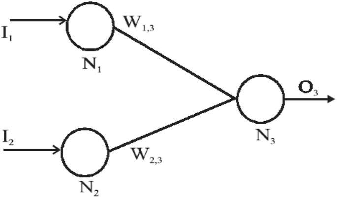
The network of PP with three neurons
where Cr is the crenel function, which is defined as follows.
where T1 and T2 are the threshold of the neuron N1 and N2.
The crenel function of the PP is given as follows (Fig. 6).

The crenel function of PP
The weights W1,3 and W2,3 can be taken as follows.
The XOR function calculation by PP is shown in Table 1.
We can adopt the following rule for changing periodicity of the activation function.
Let \(f_{r}^{k} (x)\) be the activation function with period 2 k. Here, \(f_{r}^{k} (x)\)=\(f_{r}^{{}} (\frac{x}{k})\) with weight matrix Wk. Based on the above facts, the following theorem is proved.
Theorem 1
Every Boolean function can be evaluated by using a periodic perceptron with three neurons.
Proof
Consider the network of the PP of three neurons as shown in Fig. 5, where the output neuron (i.e., N3) is provided by the activation function fr. The following need to be considered to compute the Boolean function f.
Here, r is determined as \(\left\{ {\begin{array}{*{20}c} {r = 0} & {{\text{if }}\phi (0,0) = 0} \\ {r = 1} & {\text{Otherwise}} \\ \end{array} } \right\}\).□
The weights W1,3 and W2,3 are selected randomly in order to satisfy Eqs. (13) and (14). As fv is a periodic (i.e., period 2), there exists an interval length l around W1,3, where Eqs. (13) and (14) are fulfilled. If [x1, x2] is the interval, where W1,3 satisfying Eq. (13) and [x3, x4] is the interval satisfying Eq. (14), then W1,3 and W2,3 sweep through these intervals and through an interval of length 2 ([x1 + x3, x2 + x4]), where fr (W1,3 + W2,3) is equals to 0 and 1 alternately.
The learning algorithm for PP is shown in Table 2, which is adopted based on the delta learning method.
4 Results and discussion
In this section, the results are computed to test the performance of the learning algorithm for PP in order to find the Boolean function. The algorithm uses the XOR function and the parity concept to get the results.
-
1.
The XOR function: In this problem, we train PP with three neurons and we compute XOR function.
-
2.
The parity problem: Let A be a set of n-bit vector. The set splits into A0 and A1, where A0 includes odd number of 0’s and Ai includes the others.
For t instance of time, let a be the learning rate and r is the correction factor and 0≤r≤1. The test results for the activation function with the delta learning rule are shown in Table 3. Periodic perceptron is used in such a way that the remaining hidden layer gives the same output. The algorithm is an efficient one for finding the Boolean function.
5 Conclusion
In this paper, we have observed that a two-layer perceptron with a periodic non-monotonous activation function can compute any Boolean function. An efficient learning algorithm for periodic perceptron has been proposed to test two realistic problems, such as the XOR function and the parity problem. The performance of PP have compared with multilayer perceptron and it has been observed that PP gives better result than the multilayer perceptron. In future, this work can be extended by adding the deep nueral network (DNN) and/or convolution neural network (CNN) concept to analyze the error.
References
Esteves JT, de Souza Rolim G, Ferraudo AS (2019) Rainfall prediction methodology with binary multilayer perceptron neural networks. Clim Dyn 52(3–4):2319–2331
Mileiko S, Shafik R, Yakovlev A, Edwards J (2019). A pulse width modulation based power-elastic and robust mixed-signal perceptron design. In: 2019 design, automation & test in Europe conference & exhibition (DATE). IEEE, pp 1603–1606
Sakar CO, Polat SO, Katircioglu M, Kastro Y (2019) Real-time prediction of online shoppers’ purchasing intention using multilayer perceptron and LSTM recurrent neural networks. Neural Comput Appl 31:6893–6908
Yamamoto AY, Sundqvist KM, Li P, Harris HR (2018) Simulation of a multidimensional input quantum perceptron. Quantum Inf Process 17(6):128
Amaral RPF, Ribeiro MV, de Aguiar EP (2019) Type-1 and singleton fuzzy logic system trained by a fast scaled conjugate gradient methods for dealing with binary classification problems. Neurocomputing 355:57–70
Struye J, Latré S (2019) Hierarchical temporal memory and recurrent neural networks for time series prediction: an empirical validation and reduction to multilayer perceptrons. Neurocomputing. https://doi.org/10.1016/j.neucom.2018.09.098
Rosenblatt F (1958) The perceptron: a probabilistic model for information storage and organization in the brain. Psychol Rev 65(6):386–408
Heidari AA, Faris H, Aljarah I, Mirjalili S (2019) An efficient hybrid multilayer perceptron neural network with grasshopper optimization. Soft Comput 23(17):7941–7958
Lima-Junior FR, Carpinetti LCR (2019) Predicting supply chain performance based on SCOR metrics and multilayer perceptron neural networks. Int J Prod Econ 212:19–38
Li Y, Tang G, Du J, Zhou N, Zhao Y, Wu T (2019) Multilayer perceptron method to estimate real-world fuel consumption rate of light duty vehicles. IEEE Access 7:63395–63402
Bhowmik M, Muthukumar P, Anandalakshmi R (2019) Experimental based multilayer perceptron approach for prediction of evacuated solar collector performance in humid subtropical regions. Renew Energy 143:1566–1580
Tang X, Zhang L, Ding X (2019) SAR image despeckling with a multilayer perceptron neural network. Int J Dig Earth 12(3):354–374
Pełka P, Dudek G (2019) Pattern-based forecasting monthly electricity demand using multilayer perceptron. In: International conference on artificial intelligence and soft computing. Springer, Cham, pp 663–672
Wang SH, Zhang Y, Li YJ, Jia WJ, Liu FY, Yang MM, Zhang YD (2018) Single slice based detection for Alzheimer’s disease via wavelet entropy and multilayer perceptron trained by biogeography-based optimization. Multimedia Tools Appl 77(9):10393–10417
Díaz-Álvarez A, Clavijo M, Jiménez F, Talavera E, Serradilla F (2018) Modelling the human lane-change execution behaviour through Multilayer Perceptrons and Convolutional Neural Networks. Transp Res Part F Traffic Psychol Behav 56:134–148
Hornik K (1991) Approximation capabilities of multilayer feedforward networks. Neural Netw 4(2):251–257
Hinton GE (1989) Connectionist learning procedures. Artif Intell 40(1–3):185–234
Brady MJ (1990) Guaranteed learning algorithm for network with units having periodic threshold output function. Neural Comput 2(4):405–408
Gioiello G, Sorbello F, Vassallo G, Vitabile S (1996) A new VLSI neural device with sinusoidal activation function for handwritten classification. In: Proceedings of 2nd international conference on neural networks and their applications, pp 238–242
Filliatre B, Racca R (1996) Multi-threshold neurones perceptron. Neural Process Lett 4(1):39–44
Hu J, Xu L, Wang X, Xu X, Su G (2018) Effects of BP algorithm-based activation functions on neural network convergence. J Comput 29(1):76–85
Du KL, Swamy MNS (2019) Multilayer perceptrons: architecture and error backpropagation. In: Neural networks and statistical learning. Springer, London, pp 97–141
Fawaz A, Klein P, Piat S, Severini S, Mountney P (2019). Training and meta-training binary neural networks with quantum computing. In: Proceedings of the 25th ACM SIGKDD international conference on knowledge discovery & data mining. ACM, pp 1674–1681
Laudani A, Lozito GM, Fulginei FR, Salvini A (2015) On training efficiency and computational costs of a feed forward neural network: a review. Comput Intell Neurosci 2015:83
Godfrey LB (2018) Parameterizing and aggregating activation functions in deep neural networks. Theses and Dissertations. University of Arkansas, Fayetteville. Retrieved from https://scholarworks.uark.edu/etd/2655
Author information
Authors and Affiliations
Corresponding author
Ethics declarations
Conflict of interest
The authors declare that they have no competing interests.
Additional information
Publisher's Note
Springer Nature remains neutral with regard to jurisdictional claims in published maps and institutional affiliations.
Rights and permissions
About this article

Cite this article
Mallick, C., Bhoi, S.K., Panda, S.K. et al. An efficient learning algorithm for periodic perceptron to test XOR function and parity problem. SN Appl. Sci. 2, 160 (2020). https://doi.org/10.1007/s42452-020-1952-8
Received:
Accepted:
Published:
DOI: https://doi.org/10.1007/s42452-020-1952-8