
Abstract
The present study is an effort to examine the capability of a differential evolution based radial basis function neural network (RBFDE) to model weekly reference evapotranspiration (ET0) as a function of climatic parameters in different agro-climatic zones (ACZs) of a moist sub-humid region in East-Central India. The ET0 computed using the empirical equation of Penman–Monteith suggested by the Food and Agricultural Organization (FAO56-PM) is considered as a target variable for investigation. The performance of the proposed RBFDE model is compared with particle swarm optimization based radial basis function (RBFPSO), radial basis function neural network (RBFNN), multilayer artificial neural network (MLANN) models and conventional empirical equations of Hargreaves, Turc, Open-Pan, and Blaney-Criddle. Weekly ET0 estimates that are obtained using RBFDE, RBFPSO, and RBFNN and MLANN are observed to be more consistent than equivalent empirical methods. For a critical analysis of simulation results, mean absolute percentage error (MAPE), root means square error (RMSE), determination coefficient (R2) and Nash–Sutcliffe efficiency factor (NSE) is computed. Low MAPE and RMSE values along with higher R2 and NSE close to 1, obtained with soft computing models exhibit that, soft computing models produce better estimates of ET0 than empirical methods. Among the soft computing models, RBFDE provides improved results as compared to RBFPSO, RBFNN, and MLANN models. This method can be extended for ET0 estimation in other ACZs.
1 Introduction
In response to atmospheric demand, soil surface evaporation and transpiration from plant occurs simultaneously in a cropping field and is termed as evapotranspiration (ET) in a combined manner [1]. Approximately two-thirds of the total precipitation is consumed by the atmosphere in the form of ET [2]. Therefore, ET is considered one of the most important water balance components for the determination of crop water requirement, length of the crop growing season, and associated agro-climatic studies. Hence, accurate measurement or estimation of ET is essential for the planning and effective implementation of irrigation and water management practices for practical applications. Accurate measurement of ET by volumetric and gravimetric lysimeter is practically very difficult because various factors affect the ET process, which includes climatic parameters, crop characteristics, soil properties, and management practices. Therefore, consumptive use of water from a uniformly distributed grass reference crop under nonlimiting conditions is estimated for practical purposes and termed as ET0 [3]. In general, ET0 is computed employing empirical equations as climatic parameters being the only factor affecting the ET process. Solar radiation, temperature, humidity, wind speed, and sunshine are the most influential climatic factors which contribute to the ET process [1]. Precise estimation of ET0 is vital for the efficient utilization of available water resources for agricultural purposes.
Several physicals, empirical equations based on radiation, temperature, mass transfer, and water budget methods have been derived in the past to determine ET0 with different input combinations of meteorological parameters. Among these empirical methods, the Penman–Monteith equation is recommended by the Food and Agricultural Organization for ET0 estimation (FAO56-PM) because of its preciseness [1]. FAO56-PM equation requires meteorological parameters such as maximum and minimum temperatures, relative humidity, sunshine hours, wind speed, and solar radiation to determine ET0. In developing countries, like India, it is invariably very difficult to obtain long term meteorological parameters to compute ET0 using the FAO56-PM model [4]. Therefore, other empirical models like Hargreaves [5], Turc [6], Open Pan [7], Blaney-Criddle [7], and Christianson [8], etc., are also in use. These empirical equations involve fewer complex variables as compared to FAO56-PM to compute ET0. However, ET0 estimates obtained using these models are not comparable with FAO56-PM as these methods yield more errors and hence their practical applications become limited [9].
To address this issue, in recent decades, researchers have successfully demonstrated the application of a variety of computational intelligence based conventional and hybrid soft computing techniques for modeling extremely complex and non-linear relationship between climatic factors and ET0 [10,11,12,13,14,15,16,17,18,19]. Improved predictions of FAO56-PM ET0 are obtained by Wen et al. [20] using a support vector machine (SVM) as compared to the artificial neural network (ANN) and empirical methods in extremely arid regions of China. Partal [21] has developed a hybrid model combining wavelet transformation and radial basis function neural network (W-RBF) that outperformed conventional RBF, wavelet-multi-linear regression (W-MLR) and empirical methods of Hargreaves and Turc for daily ET0 estimation with improved accuracy. Kisi and Demir [22] have evaluated the potential of multi-layer perceptron (MLP) with six different weight update algorithms for modeling ET0 and found MLP with the Levenberg-Marquard algorithm produced a better estimate of ETo. In a recent study, Dou and Yang [23] have recommended hybrid extreme learning machine (ELM) and adaptive neuro-fuzzy inference system (ANFIS) based models that are more robust and flexible in comparison to traditional ELM and ANFIS. Adamala [24] has reported improved generalized performance of wavelet neural network (WNN) and ANN model for estimation of ET0 as compared to linear regression (LR), wavelet regression (WR) and Hargreaves (HG) methods for the studied locations in different agro-ecological regions of India. Sanikhani et al. [25] have applied several artificial intelligence models including multi-layer perceptron (MLP), generalized regression neural network (GRNN), integrated ANFIS systems with grid partitioning (ANFIS-GP) and subtractive clustering (AFNIS-SC), radial basis neural network (RBNN) and GEP for modeling ET0 in a cross-station scenario for different locations in Turkey and demonstrated that AI-based models performed better than the empirical equation of Hargreaves-Samani (HS) and its calibrated version (CHS).
It is also observed from the literature review that researchers have successfully implemented various types of hybrid soft computing models combining conventional neural networks along with evolutionary computing algorithms for estimation of ET0. Application of nature-inspired algorithms such as genetic algorithm (GA), particle swarm optimization (PSO), artificial bee colony (ABC), etc., in combination with conventional neural networks like ANN and RBNN are investigated in some research publications for ET0 estimation [26,27,28,29,30]. A study conducted by Feng et al. [31] for estimating FAO56-PM ET0 in a humid region of Southwest China reveals that ELM and ANN optimized by genetic algorithm (GANN) has resulted in better ET0 estimates than WNN and empirical approaches of Hargreaves, Makkink, Priestley–Taylor and Ritchie models. Gocić et al. [32] have analyzed the potential of genetic programming (GP), support-vector machine-firefly algorithm (SVM-FFA), ANN, and SVM-Wavelet soft computing approaches and found SVM-Wavelet resulted in improved FAO56-PM ET0 estimates in Serbia. Mehdizadeh et al. [33] have evaluated the performance of gene expression programming (GEP) and MARS along with two SVM based hybrid models, SVM-Polynomial and SVM-RBF for estimation of monthly mean ET0 and reported SVM-RBF and MARS outperformed GEP and SVM-Poly and also performed better than 16 other empirical equations considered for comparison. However, Mattar and Alazba [34] have confirmed that the GEP model performed better than the conventional multilinear regression (MLR) approach in Egypt. Most of the soft computing models discussed above are developed under a given scenario in terms of study location, the combination of available input climatic parameters, time scale and duration of climatic data, model structure, learning parameters, and an optimization algorithm, etc. Therefore, practically it becomes very difficult to employ these models in a new location without proper calibration and validation of the model parameters.
To examine the potential of an evolutionary optimized soft computing technique, RBFNN in combination with the differential evolution algorithm (RBFDE) is introduced here for the estimation of ET0 under three different ACZs in the Chhattisgarh region of East-Central India. Differential evolution (DE) is considered because it is a simple algorithm in comparison to GA which requires intensive calculations. Due to its simplicity, DE is used in various applications [35,36,37]. Technical analysis of DE parameters, hybridization of DE with other soft computing techniques, and its practical applications have been discussed by Das et al. [38]. Different variants over state-of-the-art DE have also been presented in the literature. Among these, Hui and Suguntham [39] suggested ensemble and arithmetic recombination-based speciation DE for multimodal optimization of common benchmark problems. Ramdas et al. [40] developed a reconstructed mutation strategy for DE and applied the same with multilevel image thresholding for improved weather radar image segmentation [41]. A DE variant with multi-donor mutation strategy and annealing-base local search has been developed by Ghosh et al. [42] for optimization of Lennard-Jones potential function-based molecular clustering. The effect of DE-based constraint handling techniques has been evaluated by Biswas et al. [43] for the optimization of power flow systems. One of the authors of this investigation has also been engaged in DE based training of adaptive autoregressive moving average (ARMA) model for exchange rate forecasting [44] and development of a hybrid system using functional link artificial neural network (FLANN) and DE for Odia handwritten numeral recognition [45]. The proposed evolutionary optimized hybrid structure of RBFDE is developed and used for the first time to model FAO56-PM ET0, and therefore it may be considered as a novel scientific approach for such application. Conventional soft computing techniques like MLANN, RBFNN along with empirical methods of Hargreaves, Turc, Open Pan, and Blaney-Criddle are considered for comparison purposes. Results obtained with RBFDE is also compared with RBFPSO under similar condition. This paper is organized into different sections. Section 1 introduces the problem formulation, literature reviews, and motivation behind the investigation. The detailed description of the data sets, soft computing techniques, and empirical methods are described in the Materials and methods of Sect. 2. Simulation results and comparative performance evaluation of different models are outlined in the results and discussion of Sect. 3. The salient findings of the study are summarized in the conclusion section.
2 Materials and methods
2.1 Study area and dataset
This investigation is carried out to model weekly ET0 using soft computing techniques. Long term weekly meteorological data (2001 to 2019) of maximum temperature (Tmax), minimum temperature (Tmin), bright sunshine hours (BSS), wind speed (WS), morning relative humidity during (RH1), afternoon relative humidity (RH2) and weekly cumulative pan evaporation (EP) are collected from Raipur, Jagdalpur and Ambikapur stations located in three distinct ACZs of Chhattisgarh region in central India (Fig. 1). The climate of Chhattisgarh is moist sub-humid in general with an average annual rainfall of 1200–1400 mm and annual ET0 losses between 1400 and 1600 mm in different ACZs. Data sets are collected from the India Meteorological Department (IMD) (https://mausam.imd.gov.in/) certified observatories located in these stations. These surface meteorological observatories follow the World Meteorological Organization (WMO) guidelines for data collection [46]. WMO guidelines for the observational procedure and quality control are adopted uniformly in these surface meteorological observatories while data acquisition, tabulation, and computation. The online data entry system, itself has an inbuilt quality control mechanism to test the errors like data format, duplicate records, and incorrect units of measurement, impossible values, extremes, and outliers.

Location map of the study area
Descriptive statistics of different meteorological parameters in terms of mean, high, low, range, standard deviation (SD), and coefficient of variation (CV) are also computed to understand data patterns and to ensure the quality check of data (Table 1). To measure the strength and direction of a linear relationship between two variables, correlation coefficient (R) between meteorological parameters (Tmax. Tmin, BSS, WS, RH1, RH2, and EP) with FAO56-PM ET0 are also computed (Table 1). Weekly totals of ET0 are computed using the FAO56-PM equation which is considered as the target output for model development [1].
The pattern of different meteorological parameters considered as input variables for model development along with target variable FAO56-PM ET0 in selected stations is represented as box plot arrangements in Fig. 2. The middle line of the box plot signifies the median value while the upper and lower edges signify 75% and 25% of the data set respectively. The highest and lowest limits of the upper and lower vertical lines indicate the highest and lowest values respectively. The square depicts the simulated mean, and the straight-line shows the observed mean.

Box plot of input meteorological parameters and FAO56-PM ET0 in different stations
2.2 Design of soft computing models
2.2.1 Radial basis function neural network (RBFNN) based estimator
RBFNN is a category of feed-forward neural network with a single hidden layer and an output layer formulated by Broomhead and Lowe [47]. Pictorial representation of the RBFNN is given in Fig. 3. The processing units termed as neurons in the hidden layer are associated with centers, \(c = c_{1} ,c_{2} ,c_{3} ,.,.,c_{h} ,\) and their width \(\sigma = \sigma_{1} ,\sigma_{2} ,\sigma_{3} ,.,.,.\sigma_{h} ,\) where h is the number of neurons in the hidden layer. Each neuron in the hidden layer receives the same set of input data \(\left( {X = x_{1} ,x_{2} ,x_{3} ,.,.,.,x_{n} } \right).\) The centers of every hidden neuron have the same dimension as that of the input data, i.e. \(c_{i } \in R^{n} ,X \in R^{n} .\) The output of hidden layer neurons \(\left( {\varphi_{1} ,\varphi_{2} ,\varphi_{3} ,.,.,.,\varphi_{h} } \right)\) are associated with synaptic weights \(\left( {w_{1} ,w_{2} ,w_{3} ,.,.,.,w_{h} } \right).\) Output, \(\emptyset_{i}\) of ith hidden layer neuron is basically a Gaussian function and is represented by:
where \(z = \left| {\left| {x - c_{i} } \right|} \right|,\) represents the Euclidian distance between input data and the corresponding centers and \(\emptyset_{i} = \emptyset \left( {\left| {\left| {X - c_{i} } \right|} \right|} \right)\). The Gaussian function used in each hidden layer neuron is a category of radial basis function. Finally, the response of the RBFNN at the output layer, for a given set of input data is linear in terms of weights and computed using the following expression.
Development of the RBFNN for each instant of input data and its corresponding output {X, y} is obtained recursively by updating the network parameters \(\left\{ {w_{i} , c_{i} , \sigma_{i} } \right\}\) to minimize the instantaneous error cost function given as.
The weight update rules to optimize the network parameters \(\left\{ {w_{i} , c_{i} , \sigma_{i} } \right\}\) at time t are given by following equations which are derived using gradient descent algorithm [48].
where yd desired output or target value, cij jth element of the ith center, η1, η2, η3 learning rates for network parameters \(\left\{ {w_{i} , c_{i} , \sigma_{i} } \right\}\) respectively.

Block diagram of RBFNN based estimator
2.2.2 Differential evolution based RBF neural network estimator
Differential evolution (DE) [49, 50] is a simple and efficient global optimization technique based on a heuristic method for minimizing a nonlinear function. Using this efficient heuristic approach a hybrid structure, RBFDE is developed in which total d number of network parameters, represented by a parameter vector, \(\vec{x}_{i} = \left\{ {w_{i} , c_{i} , \sigma_{i} } \right\}\), is optimized by the differential evolution algorithm (DE). DE algorithm involves three basic operations viz., mutation, recombination, and selection. The step-wise procedure for the development of RBFDE is described below.
-
Step 1 Randomly initialize \(i = 1,2,3,.,.,.NP\) number of target or population vectors, \(\vec{x}_{i, G}\) between 0 to 1, where each ith individual of the population vector represents parameters of the RBFDE model. The ith target vector of Gth generation, \(\vec{x}_{i,G}\) is given as \(\vec{x}_{i, G} = \left\{ {w_{i} , c_{i} , \sigma_{i} } \right\}.\)
-
Step 2 Repeat step 3 with each target vector \(\vec{x}_{i, G}\) for \(i = 1, 2,3,.,.,.NP\).
-
Step 3 a) Give K numbers of input patterns to the RBF network sequentially with each pattern having dimension n.
b) For each one of the K input patterns, obtain corresponding network output using ith target vector \(\vec{x}_{i,G}\) as the parameters of the network and compare it with the corresponding desired output to get an error using (3). For K patterns, the K number of error values will be obtained.
c) Calculate \(f\left( {\vec{x}_{i,G} } \right)\) using (7), where \(f\left( {\vec{x}_{i,G} } \right)\) represents the fitness function i.e. mean square error (MSE).
$$f\left( {\vec{x}_{i,G} } \right) = \frac{{\mathop \sum \nolimits_{j = 1}^{K} e^{2} }}{K}$$(7) -
Step 4 Obtain \(f_{min} \left( {\vec{x}_{i,G} } \right)\) and represent the corresponding \(\vec{x}_{i,G }\) as the \(\vec{x}_{best, G}\) for Gth generation.
-
Step 5 Choose a scaling factor F \(\in \left[ {o, 1} \right]\) and a cross over ratio CR, \(\in \left[ {o, 1} \right]\) and repeat step 6 to step 15 until the desired minimum MSE is obtained.
-
Step 6 Repeat the steps from 7 to 8 for \(i = 1, 2,3,.,.,.NP\) times
-
Step 7 Randomly choose two indices \(r_{1} , r_{2}\) from 1 to NP, such that, \(r_{1} \ne r_{2} \ne i\).
-
Step 8 Compute the mutant vector \(v_{i,G}\) for each target vector \(\vec{x}_{i,G }\) for Gth generation as
$$\vec{v}_{i,G} = \vec{x}_{i,G} + F*\left( {\vec{x}_{{r_{1, G} }} - \vec{x}_{{r_{2} , G }} } \right) + F*\left( {\vec{x}_{best,G} - \vec{x}_{i,G} } \right).$$(8) -
Step 9 Repeat the steps from 10 to 11 for \(i = 1, 2,3,.,.,.NP\) times
-
Step 10 Randomly choose an index \(r_{3}\) between 1 to d and repeat step 11 for j = 1 to d, where d is the dimension of the target or population vector.
-
Step 11 Generate a random number rand \(\in \left[ {o, 1} \right]\) and compute the trial vector \(\vec{U}_{j,i, G }\) by recombination operation, which replaces the previously successful individuals with mutant vector as
$$\vec{U}_{j,i, G } = \left\{ {\begin{array}{*{20}l} {\vec{v}_{j,i, G} \;\;\;if\left( {rand \le CR} \right)\;or\;j = r_{3} } \hfill \\ {else} \hfill \\ {\vec{x}_{j, i, G} } \hfill \\ \end{array} } \right..$$(9) -
Step 12 For each trial vector \(\vec{U}_{j,i, G ,} i = 1, 2,3,.,.,.NP\), evaluate \(f\left( {U_{i, G } } \right)\), which is a mean square error (MSE). (Similar to step 3)
-
Step 13 Repeat the step14 for \(i = 1, 2,3,.,.,.NP\)
-
Step 14 Finally, the next generation of NP number of target/population vector \(\vec{x}_{i, G + 1}\) is selected based on survival of the fittest criteria as
$$\vec{x}_{i,G + 1} = \left\{ {\begin{array}{*{20}l} {\vec{U}_{i, G }\;\; \;if\;f\left( {\vec{U}_{i, G } } \right) \le f\left( { \vec{x}_{i, G} } \right)} \hfill \\ {else} \hfill \\ {\vec{x}_{i, G} } \hfill \\ \end{array} } \right..$$(10) -
Step 15 Obtain \(f_{min} \left( {\vec{x}_{i, G + 1} } \right)\) and represent it as \(\vec{x}_{best, G + 1}\) for the next generation.
-
Step 16 Stop
Pictorial representation of the DE algorithm is shown in Fig. 4.

Flowchart differential evolution algorithm
2.2.3 Particle swarm optimization based RBF neural network estimator
In this approach parameters of the RBFNN model i.e. {wi, ci, σi}, as described in Sect. 2.2.1, are updated using the PSO algorithm. The PSO [51,52,53] is a metaheuristics optimization algorithm inspired by the paradigm of swarm intelligence which mimics the social behavior of animals like fish and birds. It is successfully applied to various applications in engineering and science [54,55,56]. The algorithm uses a fixed number of particles that represent the parameters of RBFNN. Each particle updates its current velocity and position by its own experience called personal best (p-best) and by the social experience of the swarm called global best (g-best). Steps involved in PSO are briefly described below:
-
Step 1 Initialize fix number of particles with random position and velocity uniformly distributed over the search space.
-
Step 2 Evaluate the fitness of each particle according to the objective function
-
Step 3 Record pbest for each particle and g-best of the swarm.
-
Step 4 Update velocity of each particle
-
Step 5 Update the position of each particle.
-
Step 6 Update pbest and gbest
-
Step 7 Repeat the steps from 2 to 6 until the termination condition is satisfied and stop.
Pictorial representation of the PSO algorithm is shown in Fig. 5.

Flowchart particle swarm optimization algorithm
2.2.4 Multi-layer artificial neural network (MLANN)
MLANN, suggested by Haykin [57] is successfully employed in many applications to solve the regression problem. MLANN architecture considered for this proposed investigation consists of an N-5-1 structure. N represents the number of input features. Optimum results are obtained with 5 neurons in the intermittent hidden layer. Desired ET0 estimates are obtained at output neurons. Hyperbolic tangent (tanh) is used as an activation function in every processing neuron. The training of the network is done by a conventional back-propagation algorithm which is based on the error-correcting learning rule to update the weights and bias of each neuron in different layers.
2.3 Empirical models
Weekly ET0 for the study locations is also computed using empirical methods of FAO56-PM, Blaney-Criddle, Open Pan, Turc, and Hargreaves from available meteorological data. A brief description regarding empirical approaches considered in this investigation and the corresponding input meteorological parameter requirement are listed in Table 2. The description regarding different climate based empirical methods considered in this investigation is not included in this paper. More details regarding these empirical approaches can be obtained from basic references [1, 5,6,7].
2.4 Performance evaluation measures
Comparative analysis of estimated ET0 obtained with different soft computing models and empirical methods considered for the investigation is carried out by computing performance evaluation measures, namely, mean square percentage error (MAPE), root mean square error (RMSE), determination coefficient (R2) and efficiency factor (EF) proposed by Nash and Sutcliffe (NSE) [58]. The mathematical expression of different evaluation measures is as follows.
where \(Out_{obs}\) denotes the target and \(Out_{est}\) denotes model estimated ET0 values. n is the number of testing patterns. Low MAPE and RMSE values represent the close agreement between desired and estimated output. Similarly, R2 and EF values close to 1 are also indicators of a higher accuracy level of the model.
3 Results and discussion
The key objective of this investigation is to examine the potential of different evolutionary optimized hybrid (RBFDE, RBFPSO) and conventional (RBFNN, MLANN) soft computing approaches with available climatic features for estimation of ET0 comparable to FAO56-PM ET0. Input features combination of different models is decided based on empirical approaches of Hargreaves, Turc, Open Pan, Blaney-Criddle, and FAO56-PM ET0 listed in the previous section. These soft computing models are categorized into type I to type V models. Like the Hargreaves method, type I models include only Tmax and Tmin as input features, whereas Type II soft computing models include BSS with temperature, which is equivalent to the Turc approach. In type III soft computing models, EP, RH1, RH2, and WS are considered as input features similar to that of the Open Pan empirical approach. Type IV models include six weather parameters (Tmax, Tmin, BSS, WS, and RH1 and RH2) equivalent to the Blaney-Criddle empirical approach. Another category of soft computing model termed Type V models are developed using Tmax, Tmin, BSS, and WS since these weather parameters exhibit positive correlations with ET0. The input feature EP, which is also positively correlated with ET0, is not included in type V soft computing models as obtaining EP data is very difficult. Input feature combinations used in different types of soft computing models and their equivalent empirical models are shown in Table 3. Weekly meteorological data of Raipur, Jagdalpur, and Ambikapur from 2001 to 2015 (80%) are used for model calibration or training, whereas the recent 4 years (20%) of the weekly meteorological data from 2016 to 2019 are used for model validation.
Soft computing models RBFDE, RBFPSO, RBFNN, and MLANN are coded in MATLAB as per the design and the learning algorithm described earlier. Simulation studies are carried out with a different input features combination to test the sensitivity of the soft computing approach to control parameters until a satisfactory accuracy level is achieved for estimation of FAO56-ET0 for different study locations. Detailed information regarding modeling strategies and respective control parameters that produce optimum results during the simulation process are shown in Table 4 for different soft computing models.
Calibration of RBFDE, RBFPSO, RBFNN, and MLANN models is done using the above-listed network parameters with training datasets of all the three study locations, Raipur, Jagdalpur, and Ambikapur. During the training process, input patterns are given to the model sequentially and the corresponding estimated output is obtained at the output layer after completion of the forward pass (Fig. 3). The estimated output is compared with the corresponding target FAO56-ET0 output to compute the instantaneous error cost function. Real-time update of the model parameters is done in each instance to minimize the squared error using respective evolutionary (DE and PSO) and conventional back-propagation learning algorithms (RBFNN and MLANN). The process continues until all the available training input patterns for model calibration gets exhausted. This completes one cycle called an epoch. At the end of each epoch, the mean square error is computed and stored for each epoch to examine the learning characteristic of soft computing models. The iterative process is repeated several times until MSE is minimized to a desired low value nearly close to zero. This completes the supervised learning process and model parameters are then fixed to constitute soft computing models. A similar calibration process is adopted for all soft computing approaches.
To test the performance of different soft computing models, test data patterns are then presented sequentially at the input layer of the model and through forward pass respective estimated ET0 is obtained at the output layer for all the test patterns. These ET0 estimates are then compared with corresponding target FAO56-PM ET0 values. Performance evaluation measures, MAPE (%), RMSE (mm week−1), R2, and NSE as described in the previous section are then computed using desired and estimated output of different types of soft computing models and equivalent empirical approaches for comparison of model performance, which ultimately leads to model selection. The computed values of performance evaluation measures for different types of soft computing models and equivalent empirical approaches considered are listed in Tables 5 and 6 for all three locations. Comparative results of the analysis are discussed below:
-
i.
For type I soft computing models, MAPE ranges from lowest of 7.4 for RBFDE1 and RBFDE2 (at Raipur) to highest of 11.8 for MLANN1 (at Jagdalpur), whereas MAPE obtained with Hargreaves model is comparatively very high and ranges between 22.6 (at Raipur) to 30.3 (at Ambikapur).
-
ii.
Type II soft computing models produce improved ET0 estimates with low MAPE compared to type I models. For type II models, MAPE ranges from the lowest of 4.9 with RBFDE2 (at Raipur) to a high of 10.2 with MLANN2 (at Raipur). MAPE is again quite higher with the equivalent empirical approach of Turc, which is obtained between 10.1 (at Jagdalpur) to 13.9 (at Raipur).
-
iii.
Subsequently, for type III models, MAPE values are computed close to that of type II models, which varied between a lowest of 4.7 with RBFDE3 & RBFPSO3 (at Raipur) to a high of 8.0 with MLANN3 (at Jagdalpur). MAPE for the Open Pan approach varies between 12.2 (at Raipur) to 22.2 (at Ambikapur), which is very high as compared to type III soft computing models.
-
iv.
Type IV soft computing models yield better results as compared to all other types of soft computing and empirical models. MAPE ranges between a low of 1.1 to a high of 3.9 at Raipur, followed by 3.7 to 4.4 at Jagdalpur and 2.2 to 4.6 at Ambikapur with RBFDE4 and MLANN4 respectively. MAPE with the Blaney-Criddle method is again quite inferior as compared to type IV soft computing approaches and ranges from 15.5 (at Jagdalpur) to 22.6 (at Raipur).
-
v.
Type V models also produced good results, as reasonably fair estimates of ET0 can be obtained between a low MAPE of 1.9 with RBFDE5 (at Raipur) to 5.2 with MLANN5 (at Jagdalpur and Ambikapur), which is very much comparable to that of type IV models, even without taking humidity data as one of the input features.
-
vi.
Regarding RMSE, type I soft computing models have resulted in RMSE between 2.98 mm week−1 (at Raipur) with RBFDE1 and RBFPSO1 to 3.88 week−1 (at Jagdalpur) with MLANN1, as against the higher RMSE of 6.13 week−1 (at Raipur) to 7.53 mm week−1 (at Jagdalpur) obtained with Hargreaves approaches.
-
vii.
Type II soft computing models have produced improved RMSE as compared to type I models, which ranges between a low of 2.10 mm week−1 with RBFDE2 (at Ambikapur) to a high of 3.45 mm week−1 with MLANN2 (at Raipur). Interestingly, at Jagdalpur the soft computing models produce comparatively better estimates of FAO56-PM ET0 in terms of RMSE as compared with similar models at Jagdalpur and Raipur. In general, type II soft computing models have yielded better ET0 estimates as compared to Turc methods, for which RMSE ranges between 3.73 (at Ambikapur) to 6.54 mm week−1 (at Raipur).
-
viii.
Regarding type III models, RMSE has improved further and is computed between a low of 1.75 mm week−1 with RBFDE3 to a high of 2.28 mm week−1 with MLANN3 at Raipur, whereas the same for Jagdalpur and Ambikapur, it varied between a low of 1.82 mm week−1 with RBFDE3 to a high of 2.48 mm week−1 with MLANN3. The equivalent empirical method of Open Pan has produced higher RMSE, which varied between 5.05 mm week−1 in Raipur to 6.55 mm week−1 at Ambikapur, which is almost three times more as compared to type III soft computing models.
-
ix.
Similar to MAPE, type IV soft computing models have yielded excellent results in terms of RMSE also. In Raipur, RMSE ranges between the lowest of 0.36 mm week−1 with RBFDE4 to the highest of 1.29 mm week−1 with MLANN4. At Jagdalpur, it ranges between 1.06 mm week−1 with RBFDE4 to 1.25 mm week−1 with MLANN4, whereas at Ambikapur, RMSE ranges between 0.68 mm week−1 with RBFDE4 to 1.36 mm week−1 with MLANN4. The low RMSE values (< 1 mm week−1) obtained with evolutionary optimized hybrid soft computing models (RBFDE4 and RBFDE5) are quite encouraging. This demonstrates the potential of the RBFDE4 and RBFPSO4 models and these models may consider as an alternative to the FAO56-PM empirical approach for ET0 estimation in the study area. In contrast, Blaney-Criddle has produced very high RMSE, which ranges between 4.27 to 7.29 mm/week at different locations, similar to that of the Open Pan method.
-
x.
Type V, soft computing models have also produced better results which is quite identical with type IV models even without including humidity data as an input feature. RMSE with type V models ranges between lowest 0.66 mm week−1 with RBFDE5 to highest of 1.48 mm week−1 with MLANN5 at Ambikapur. At Raipur and Jagdalpur, RMSE ranges between 0.80 to 1.31 and 1.06 to 1.46 mm week−1 with RBFDE5 and MLANN5 models respectively.
To further examine the relationship between the estimated and FAO56-PM ET0, two more statistical measures, R2 and NSE are computed for different soft computing and empirical models and shown in Table 6. The linear relationship between estimated ET0 and FAO56-ET0 is also depicted in Figs. 6, 7, and 8 in Ambikapur, Jagdalpur, and Raipur respectively. In general, both R2 and NSE convey similar information about the model performance and therefore, the marginal difference is observed between these two performance evaluation measures within a similar type of model in different locations. However, sometimes R2 values give a false indication and produce higher values close to 1 despite a very high intercept. In such cases corresponding NSE helps in evaluating the model performance.
Fig. 6 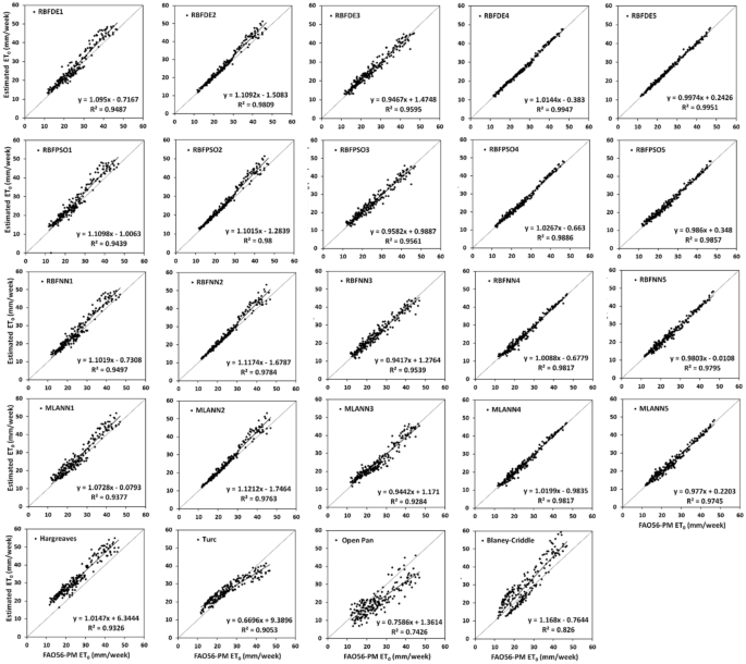
Relationship between estimated ET0 and FAO56-PM ET0 for different soft computing and empirical models with test data sets at Ambikapur
Fig. 7 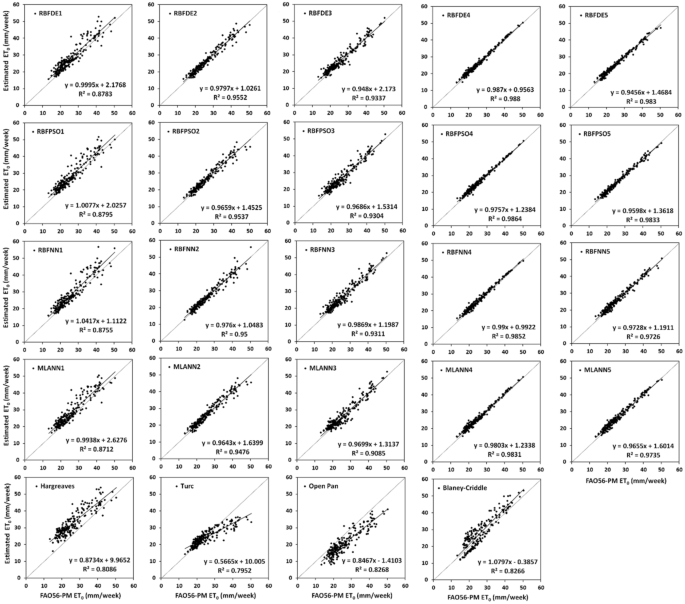
Relationship between estimated ET0 and FAO56-PM ET0 for different soft computing and empirical models with test data sets at Jagdalpur
Fig. 8 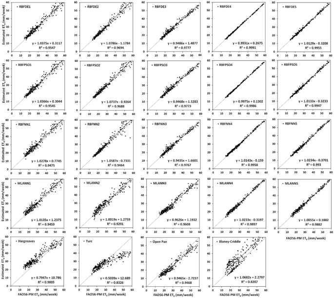
Relationship between estimated ET0 and FAO56-PM ET0 for different soft computing and empirical models with test data sets at Raipur
-
xi.
Type IV soft computing models have produced better R2 and NSE values as compared to all other models considered for investigation. The highest R2 values of 0.999, 0.988, and 0.995 are obtained with RBFDE4 and RBFPSO4 in Raipur, Jagdalpur, and Ambikapur respectively with test data sets. The remaining type IV soft computing models also produced good R2 and NSE values as compared to the equivalent empirical approach.
-
xii.
Similar results are obtained with type V soft computing models, as R2 and the corresponding NSE vary between 0.965 to 0.996 in different locations, with RBFDE5 and RBFPSO5 being the best models.
-
xiii.
For the type III model, R2 and NSE range between 0.961 to 0.978 at Raipur and between 0.900 to 0.960 at Jagdalpur and Ambikapur. R2 and NSE with type II soft computing models vary between 0.910 to 0.981. Hence, it can be stated that consistent ET0 estimates with a fair degree of agreement between estimated and target ET0 can be obtained using Type both II and III soft computing models.
-
xiv.
Type I soft computing models of RBFDE1 and RBFPSO1 have resulted in slightly lower R2 and NSE values than RBFNN1 and MLANN1 as compared to remaining types mainly as fewer input features are involved in computations.
-
xv.
Inconsistence and low R2 and NSE values that have obtained with empirical approaches of Hargreaves, Turc, Open Pan, and Blaney Criddle as compared to their equivalent soft computing models of respective types, clearly establish the fact that soft computing models produce better estimates of FAO56-PM ET0 than empirical models.


Results of the performance evaluation analysis indicate that the evolutionary optimized hybrid soft computing models considered for the investigation (RBFDE and RBFPSO) performed consistently better than other conventional soft computing techniques (RBFNN and MLANN) and empirical approaches in all the objectives. From the inferences, it is also evident that when a complete set of the climatic variable is involved in the computation of ET0 using these models, it looks very difficult to choose between RBFDE and RBFPSO as they look statistically similar in some cases. However, the proposed RBFDE is recommended because of its preciseness and generalization performance in estimating ET0 in all the stations considered for the study.
4 Conclusions ET0
The present investigation is carried out to examine the generalized potential of evolutionary optimized hybrid soft computing techniques RBFDE and RBFPSO for the estimation of ET0 in different ACZs. The ET0 estimates obtained with proposed RBFDE and RBFPSO models are compared to the conventional neural network (RBFNN, MLANN) and existing empirical approaches. Looking to the scarcity of complete datasets required for computation of FAO-PM ET0, four variants of each category of soft computing models (RBFDE, RBFPSO, RBFNN, and MLANN) equivalent (in terms of input feature combination) to empirical approaches (Hargreaves, Turc, Open Pan and Blaney-Criddle) is examined. It can be concluded that different soft computing models considered in this investigation, have resulted in improved and more consistent FAO56-PM ET0 estimates as compared to equivalent empirical approaches. Among the soft computing models, evolutionary models RBFDE and RBFPSO produced a more precise estimation of FAO56-PM ET0 than conventional RBFNN and MLANN as proposed RBFDE and RBFPSO models resulted in low MAPE and RMSE and high R2 and NSE close to 1 in most of the cases. However, ET0 estimates obtained with the proposed RBFDE seems to be slightly better than RBFPSO. Hence, appropriate soft computing models may be recommended for the estimation of ET0 in other stations of respective ACZs of the study area. The proposed soft computing models may be embedded in crop weather simulation models as subroutines for precise estimation ET0 with available input features. However, re-calibration and re-validation of these data-driven models are essentially required for their effective implantation in other parts of the world.
References
Allen RG, Pereira LS, Raes D, Smith M (1998) Introduction to evapotranspiration. In: Crop evapotranspiration-guidelines for computing crop water requirements-FAO Irrigation and drainage paper, vol 56, pp 1–13. FAO, Rome. https://doi.org/10.1016/j.eja.2010.12.001
Elizabeth AH, Robert EC (2013) Water balance estimates of evapotranspiration rates in areas with varying land use. In: Evapotranspiration-an overview. InTech. https://doi.org/10.5772/52811
Allen RG, Jensen ME, Wright JL, Burman RD (1989) Operational estimates of reference evapotranspiration. Agron J 81(4):650–662. https://doi.org/10.2134/agronj1989.00021962008100040019x
Droogers P, Allen RG (2002) Estimating reference evapotranspiration under inaccurate data conditions. Irrigat Drain Syst 16(1):33–45. https://doi.org/10.1023/A:1015508322413
Hargreaves GL, Hargreaves GH, Riley JP (1985) Agricultural, benefits for Senegal River Basin. J Irrig Drain Eng ASCE 111:113–124
Turc L (1961) Evaluation des besoins en eau d’irrigation, evapotranspiration potentielle, formule climatique simplifice et mise a jour. Ann Agron 12:13–49 (in French)
Doorenbos J, Pruitt WO (1977) Guidelines for predicting crop water requirements. Irrigation and drainage paper No 24, 2nd edn, Food and Agriculture Organization, Rome, p 156
Christiansen JE (1968) Pan evaporation and evapotranspiration by climatic data. J Irrig Drain Div Am Soc Civil Eng 94:243–263
Bapuji RB, Sandeep VM, Rao VUM, Venkateswarlu B (2012) Potential Evapotranspiration estimation for Indian conditions: Improving accuracy through calibration coefficients. Technical Bull No 1/2012. All India Co-ordinated Research Project on Agrometeorology, Central Research Institute for Dryland Agriculture, Hyderabad, p 60
Chauhan S, Shrivastava RK (2009) Performance evaluation of reference evapotranspiration estimation using climate based methods and artificial neural networks. Water Resour Manag 23(5):825–837
Kisi O, Guven A (2010) Evapotranspiration modeling using linear genetic programming technique. J Irrig Drain Eng 136(10):715–723. https://doi.org/10.1061/(asce)ir.1943-4774.0000244
Kumar M, Raghuwanshi NS, Singh R (2011) Artificial neural networks approach in evapotranspiration modeling: a review. Irrig Sci. https://doi.org/10.1007/s00271-010-0230-8
Mallikarjuna P, Jyothy SA, Sekhar Reddy KC (2012) Daily reference evapotranspiration estimation using linear regression and ANN models. J Inst Eng Ser A 93(4):215–221. https://doi.org/10.1007/s40030-013-0030-2
Kisi O (2016) Modeling reference evapotranspiration using three different heuristic regression approaches. Agric Water Manag 169:162–172. https://doi.org/10.1016/j.agwat.2016.02.026
Yassin MA, Alazba AA, Mattar MA (2016) Artificial neural networks versus gene expression programming for estimating reference evapotranspiration in an arid climate. Agric Water Manag 163:110–124. https://doi.org/10.1016/j.agwat.2015.09.009
Antonopoulos VZ, Antonopoulos AV (2017) Daily reference evapotranspiration estimates by artificial neural networks technique and empirical equations using limited input climate variables. Comput Electron Agric 132:86–96. https://doi.org/10.1016/j.compag.2016.11.011
Nema MK, Khare D, Chandniha SK (2017) Application of artificial intelligence to estimate the reference evapotranspiration in sub-humid Doon valley. Appl Water Sci 7(7):3903–3910. https://doi.org/10.1007/s13201-017-0543-3
Pandey PK, Nyori T, Pandey V (2017) Estimation of reference evapotranspiration using data-driven techniques under limited data conditions. Model Earth Syst Environ 3(4):1449–1461. https://doi.org/10.1007/s40808-017-0367-z
Patil AP, Deka PC (2017) Performance evaluation of hybrid Wavelet-ANN and Wavelet-ANFIS models for estimating evapotranspiration in arid regions of India. Neural Comput Appl 28(2):275–285. https://doi.org/10.1007/s00521-015-2055-0
Wen X, Si J, He Z, Wu J, Shao H, Yu H (2015) Support-vector-machine-based models for modeling daily reference evapotranspiration with limited climatic data in extreme arid regions. Water Resour Manag 29(9):3195–3209. https://doi.org/10.1007/s11269-015-0990-2
Partal T (2016) Comparison of wavelet-based hybrid models for daily evapotranspiration estimation using meteorological data. KSCE J Civil Eng 20(5):2050–2058. https://doi.org/10.1007/s12205-015-0556-0
Kisi O, Demir V (2016) Evapotranspiration estimation using six different multi-layer perceptron algorithms. Irrig Drain Syst Eng. https://doi.org/10.4172/2168-9768.1000164
Dou X, Yang Y (2018) Evapotranspiration estimation using four different machine learning approaches in different terrestrial ecosystems. Comput Electron Agric 148:95–106. https://doi.org/10.1016/j.compag.2018.03.010
Adamala S (2018) Temperature based generalized wavelet-neural network models to estimate evapotranspiration in India. Inf Process Agric 5(1):149–155. https://doi.org/10.1016/j.inpa.2017.09.004
Sanikhani H, Kisi O, Maroufpoor E, Yaseen ZM (2018) Temperature-based modeling of reference evapotranspiration using several artificial intelligence models: application of different modeling scenarios. Theoret Appl Climatol 135(1–2):449–462. https://doi.org/10.1007/s00704-018-2390-z
Ozkan C, Kisi O, Akay B (2011) Neural networks with artificial bee colony algorithm for modeling daily reference evapotranspiration. Irrig Sci 29(6):431–441. https://doi.org/10.1007/s00271-010-0254-0
Eslamian SS, Gohari SA, Zareian MJ, Firoozfar A (2012) Estimating Penman-Monteith reference evapotranspiration using artificial neural networks and genetic algorithm: a case study. Arab J Sci Eng 37(4):935–944. https://doi.org/10.1007/s13369-012-0214-5
Aghajanloo MB, Sabziparvar AA, Hosseinzadeh TP (2013) Artificial neural network-genetic algorithm for estimation of crop evapotranspiration in a semi-arid region of Iran. Neural Comput Appl 23(5):1387–1393. https://doi.org/10.1007/s00521-012-1087-y
Petković D, Gocic M, Shamshirband S, Qasem SN, Trajkovic S (2016) Particle swarm optimization-based radial basis function network for estimation of reference evapotranspiration. Theoret Appl Climatol 125(3–4):555–563. https://doi.org/10.1007/s00704-015-1522-y
Jovic S, Nedeljkovic B, Golubovic Z, Kostic N (2018) Evolutionary algorithm for reference evapotranspiration analysis. Comput Electron Agric 150:1–4. https://doi.org/10.1016/j.compag.2018.04.003
Feng Y, Cui N, Zhao L, Hu X, Gong D (2016) Comparison of ELM, GANN, WNN and empirical models for estimating reference evapotranspiration in the humid region of Southwest China. J Hydrol 536:376–383. https://doi.org/10.1016/j.jhydrol.2016.02.053
Gocić M, Motamedi S, Shamshirband S, Petković D, Ch S, Hashim R, Arif M (2015) Soft computing approaches for forecasting reference evapotranspiration. Comput Electron Agric 113:164–173. https://doi.org/10.1016/j.compag.2015.02.010
Mehdizadeh S, Behmanesh J, Khalili K (2017) Using MARS, SVM, GEP and empirical equations for estimation of monthly mean reference evapotranspiration. Comput Electron Agric 139:103–114. https://doi.org/10.1016/j.compag.2017.05.002
Mattar MA, Alazba AA (2018) GEP and MLR approach for the prediction of reference evapotranspiration. Neural Comput Appl. https://doi.org/10.1007/s00521-018-3410-8
Baltzis K (2013) Patented applications of differential evolution in microwave and communication engineering. Recent Patents Comput Sci 6(2):115–128. https://doi.org/10.2174/22132759113069990004
Tenaglia GC, Lebensztajn L (2014) A multiobjective approach of differential evolution optimization applied to electromagnetic problems. IEEE Trans Magn. https://doi.org/10.1109/TMAG.2013.2285980
Uher V, Gajdoš P, Radecký M, Snášel V (2016) Utilization of the discrete differential evolution for optimization in multidimensional point clouds. Comput Intell Neurosci. https://doi.org/10.1155/2016/6329530
Das S, Abraham A, Konar A (2008) Particle swarm optimization and differential evolution algorithms: technical analysis, applications and hybridization perspectives. Stud Comput Intell 116:1–38. https://doi.org/10.1007/978-3-540-78297-1_1
Hui S, Suganthan PN (2016) Ensemble and arithmetic recombination-based speciation differential evolution for multimodal optimization. IEEE Trans Cybern 46(1):64–74. https://doi.org/10.1109/TCYB.2015.2394466
Ramadas M, Abraham A, Kumar S (2018) RDE reconstructed mutation strategy for differential evolution algorithm. Adv Intell Syst Comput 614:76–85. https://doi.org/10.1007/978-3-319-60618-7_8
Ramadas M, Pant M, Abraham A, Kumar S (2019) Segmentation of weather radar image based on hazard severity using RDE: reconstructed mutation strategy for differential evolution algorithm. Neural Comput Appl 31:1253–1261. https://doi.org/10.1007/s00521-017-3091-8
Ghosh A, Mallipeddi R, Das S, Das AK (2018) A switched parameter differential evolution with multi-donor mutation and annealing based local search for optimization of lennard-jones atomic clusters. In: 2018 IEEE congress on evolutionary computation, CEC 2018-Proceedings. Institute of Electrical and Electronics Engineers Inc. https://doi.org/10.1109/CEC.2018.8477991
Biswas PP, Suganthan PN, Mallipeddi R, Amaratunga GAJ (2018) Optimal power flow solutions using differential evolution algorithm integrated with effective constraint handling techniques. Eng Appl Artif Intell 68:81–100. https://doi.org/10.1016/j.engappai.2017.10.019
Rout M, Majhi B, Majhi R, Panda G (2014) Forecasting of currency exchange rates using an adaptive ARMA model with differential evolution based training. J King Saud Univ Comput Inf Sci 26(1):7–18. https://doi.org/10.1016/j.jksuci.2013.01.002
Pujari P, Majhi B (2017) Application of natured-inspired technique to Odia handwritten numeral recognition, book chapter in handbook of research on modeling, analysis and application of nature-inspired Metaheuristic algorithms, IGI Global Publication, USA, pp 377–399 https://doi.org/10.4018/978-1-5225-2857-9.ch019
World Meteorological Organization (2012) WMO-No. 8-Guide to meteorological instruments and methods of observation, pp I.8-1–I.9-1
Broomhead D, Lowe D (1988) Multivariable functional interpolation and adaptive networks. Complex Syst 2:321–355
Fernández-Redondo M, Hernández-Espinosa C, Ortiz-Gómez M, Torres-Sospedra J (2004) Training radial basis functions by gradient descent. In: Lecture notes in artificial intelligence (subseries of lecture notes in computer science), Vol 3070, pp 184–189. Springer Verlag. https://doi.org/10.1007/978-3-540-24844-6_23
Storn R, Price K (1995) Differential evolution-a simple and efficient adaptive scheme for global optimization over continuous spaces. Technical Report TR-95-012, pp 1–12 https://doi.org/10.1.1.1.9696
Storn R, Price K (1997) Differential evolution-a simple and efficient Heuristic for global optimization over continuous spaces. J Global Optim 11(4):341–359. https://doi.org/10.1023/A:1008202821328
Kennedy J, Eberhart R (1995) Particle swarm optimization. Proc IEEE Int Conf Neural Netw 4:1942–1948
Eberhart R, Kennedy J (2002) A new optimizer using particle swarm theory. In: Institute of Electrical and Electronics Engineers (IEEE), pp 39–43 https://doi.org/10.1109/mhs.1995.494215
Eberhart R, Yuhui S (2002) Particle swarm optimization: developments, applications and resources. In: Institute of Electrical and Electronics Engineers (IEEE), pp 81–86 https://doi.org/10.1109/cec.2001.934374
del Valle Y, Venayagamoorthy GK, Mohagheghi S, Hernandez JC, Harley RG (2008) Particle swarm optimization: basic concepts, variants and applications in power systems. IEEE Trans Evol Comput. https://doi.org/10.1109/TEVC.2007.896686
Chen LF, Su CT, Chen KH (2012) An improved particle swarm optimization for feature selection. Intell Data Anal 16(2):167–182. https://doi.org/10.3233/IDA-2012-0517
Zhang Y, Wang S, Ji GA (2015) Comprehensive survey on particle Swarm optimization algorithm and its applications. Mathematical Problems in Engineering, pp 1–38 https://doi.org/10.1155/2015/931256
Haykin S (1998) Neural networks–a comprehensive foundation, 2nd edn. Prentice-Hall, Upper Saddle River, pp 26–32
Nash JE, Sutcliffe JV (1970) River flow forecasting through conceptual models part I-a discussion of principles. J Hydrol 10(3):282–290
Author information
Authors and Affiliations
Corresponding author
Ethics declarations
Conflict of interest
The authors declare that they have no conflict of interest.
Ethical approval
This article does not contain any studies with human participants or animals performed by any of the authors.
Additional information
Publisher's Note
Springer Nature remains neutral with regard to jurisdictional claims in published maps and institutional affiliations.
Rights and permissions
Open Access This article is licensed under a Creative Commons Attribution 4.0 International License, which permits use, sharing, adaptation, distribution and reproduction in any medium or format, as long as you give appropriate credit to the original author(s) and the source, provide a link to the Creative Commons licence, and indicate if changes were made. The images or other third party material in this article are included in the article's Creative Commons licence, unless indicated otherwise in a credit line to the material. If material is not included in the article's Creative Commons licence and your intended use is not permitted by statutory regulation or exceeds the permitted use, you will need to obtain permission directly from the copyright holder. To view a copy of this licence, visit http://creativecommons.org/licenses/by/4.0/.
About this article

Cite this article
Majhi, B., Naidu, D. Differential evolution based radial basis function neural network model for reference evapotranspiration estimation. SN Appl. Sci. 3, 56 (2021). https://doi.org/10.1007/s42452-020-04069-z
Received:
Accepted:
Published:
DOI: https://doi.org/10.1007/s42452-020-04069-z