Modelling evaporation in electron-beam physical vapour deposition of thermal barrier coatings

Abstract

This work presents computational models of ingot evaporation for electron-beam physical vapour deposition (EB-PVD) that can be applied to the deposition and development of thermal barrier coatings (TBCs). TBCs are insulating coatings that protect aero-engine components from high temperatures, which can be above the component’s melting point. The development of advanced TBCs is fuelled by the need to improve engine efficiency by increasing the engine operating temperature. Rare-earth zirconates (REZ) have been proposed as the next-generation TBCs due to their low coefficient of thermal conductivity and resistance to molten calcium-magnesium alumina-silicates (CMAS). However, the evaporation of REZ has proven to be challenging, with some coatings displaying compositional segregation across their thickness. The computational models form part of a larger analytical model that spans the whole EB-PVD process. The computational models focus on ingot evaporation, have been implemented in MATLAB and include data from 6 oxides: ZrO₂, Y₂O₃, Gd₂O₃, Er₂O₃, La₂O₃ and Yb₂O₃. Two models (2D and 3D) successfully evaluate the evaporation rates of constituent oxides from multiple-REZ ingots, which can be used to highlight incompatibilities and preferential evaporation of some of these oxides. A third model (local composition activated, LCA) successfully predicts the evaporation rate of the whole ingot and replicates the cyclic change in composition of the evaporated plume, which is manifested as changes in compositional segregation across the coating’s thickness. The models have been validated with experimental data from Cranfield University’s EB-PVD coaters, published vapour pressure calculations and evaporation rate formulas described in the literature.

1 Introduction

The drive for increasing engine efficiency and decreasing fuel consumption are two of the biggest challenges for the aerospace industry. These had been addressed to some degree through the application of thermal barrier coatings (TBCs) and labyrinthine internal air cooling passages [1, 2]; in combination, these two features enable high pressure, high temperature (HPHT) turbine blades to operate at surface temperatures above their melting point [3]. However, additional challenges arise at even higher operating temperatures including degradation induced by ingestion of airborne particulates, known as CMAS, that melt and flux the ceramic topcoat. CMAS mainly comprise calcia, magnesia, alumina and silica, along with more minor earth oxides, iron oxides and oxides such as those of nickel and titanium arising from within the engine. These melt on the surface of the TBC at high temperatures, leading to coating damage and loss of thermal protection for the underlying substrate alloy. New TBC materials are being sought to overcome these chemical challenges. Particular classes of materials of interest for the challenge include the rare-earth zirconates and especially gadolinium zirconate, many of which undergo reactive crystallisation with CMAS forming a protective environmental barrier layer. A significant drawback for such materials is their low fracture toughness, when compared with the industry standard TBC material of 7 wt% yttria stabilised zirconia (7YSZ). This has led to much interest in the application of rare-earth zirconate TBCs modified with toughening additives, such as titania and tantala, or structurally modified to include a tough interfacial layer. Examples here include gadolinium zirconate on top of 7YSZ or gadolinium zirconate on top of a low thermal conductivity interlayer. These approaches allow the structural balance of thermal conductivity, CMAS resistance and topcoat toughness [4].

Different methods can be used to produce TBCs, but electron-beam physical vapour deposition (EB-PVD) is the most widely used for coating HPHT turbine components. EB-PVD results in columnar microstructures that have high strain tolerance under thermal cyclic conditions encountered during service duty cycles. However, significant challenges exist in evaporating such novel materials.

EB-PVD is one of a collection of coating deposition processes that comprise PVD. The different PVD techniques, such as EB-PVD, cathodic arc and sputtering, generate coatings with different properties, but all share a common physical principle. In general, a PVD process is a vacuum deposition method used for producing high-purity thin films. First, molecules are vaporised or ejected from a solid or liquid target by an energy source. Then, molecules move inside a vacuum or low-pressure chamber to the substrate by molecular flow, with some scattering at soft vacuums, where they condense to form the coating [5]. Such produced thin films have a thickness from a few to many thousands of nanometres [5]. As shown in Fig. 1, the PVD process can be divided into three main steps [6].

Fig. 1

Steps of the PVD process

In the EB-PVD process, the energy source is an electron beam, and the coating thickness produced can be of the order of hundreds of micrometres, much larger than other PVD techniques such as sputtering, as shown in Fig. 2. These thick coatings are achieved thanks to the large deposition rates that EB-PVD can produce compared to other PVD techniques. Figure 3 shows the equipment needed for the process. Electrons are accelerated by a high voltage towards the target, which is usually in ingot form, as more material is needed to deposit thicker coatings. A beam guidance system is used to focus the beam on the target, and the target material then melts to create a melt pool. If the energy is sufficient, target atoms and molecular sub-species are able to leave the melt pool and evaporate inside the chamber [7] and then condense on any available cooler surfaces, including the substrate. Ingots are held in a water-cooled hearth and screw-fed through holes to control the feed rate of target material. To obtain complex compositions, mixtures of materials or layered coatings, multiple ingots can be placed in the hearth for sequential or simultaneous evaporation. However, producing complex compositions, or even evaporating single-source novel materials, can be difficult depending on local vapour pressures and lead to inhomogeneous coatings [8]. Therefore, the development of advanced TBCs requires a prior optimisation of the evaporation process before the desired coatings can be deposited. This can be expensive due to the necessary permutations on ingot manufacture, with different compositions, and the time, energy and expense associated with multiple EB-PVD deposition campaigns.

Fig. 2

Back-scattered electron microscope image of typical columnar structure of an EB-PVD Thermal barrier coating composed of 7 wt.% yttria-stabilised zirconia. Deposited and imaged at Cranfield University

Fig. 3

Schematic diagram of EB-PVD equipment. Additional heat sources for substrate pre-heating can also be present in the form of heating elements in the chamber, heating elements in a loading chamber or a secondary electron-beam gun

The use of computer modelling could reduce the expense and time required to optimise the evaporation process and coating development overall. Most published models are concerned with prediction of coating properties, such as thermal conductivity of zirconia ceramics [9], or with estimation of reflectance and transmittance of the coating [10]. Fewer models have been developed to study the consequences of evaporation on coating morphology. One of them is the work of Baek, Prabhu et al. [11, 12], which predicts the thickness distribution of the coating from considerations of the geometry of the evaporation plume. Their work was later refined to predict the generation of diverse coating microstructures, such as zigzag and helical columnar shapes [13]. However, these models consider single materials being evaporated, whereas advanced TBC materials are composed of diverse constituents. During evaporation, these complex materials decompose into their sub-constituents, and difficulties often arise from the difference in vapour pressure of each sub-component [8].

This paper presents a model for the evaporation of multiple-component materials during the EB-PVD process, based on the deposition parameters used in the laboratory, and is validated with experimental results and published data. The model considers the energy input from the electron-beam gun, the raster pattern on the ingot surface to predict the temperature profile on the ingot and its evolution over time. 2D and 3D variants of the model are presented, each of them considering the vapour pressures of the materials considered as ingot constituents, which enables an accurate prediction of ingot consumption rates and of differential evaporation of the diverse constituents. The predictions of temperature profiles, evaporation rates and preferential evaporation are compared with experimental observations and published literature.

2 Method

2.1 Analytical model for the evaporation step

The evaporation process is divided into smaller steps that are studied to create the analytical model used for programming, as shown in Fig. 4.

Fig. 4

Flow chart of the evaporation step

2.1.1 Electron-beam settings and ingot surface temperature

The analytical model intends to replicate Cranfield University’s EB-PVD coating system (a modified Von Ardenne EBE 150, with custom designed 3-ingot hearth and jumping-beam technology). Coating deposition usually takes place in a chamber in a 90% O₂ + 10% Ar atmosphere at around 5 ∙ 10⁻³ mbar, with samples to be coated pre-heated to ~ 1030 ºC. The material to be evaporated is in the form of an ingot of 40 mm in diameter and up to 300 mm long, which rests in a water-cooled hearth, so it is not greatly affected by the pre-heat temperature. Further detail on deposition parameters and coting structure can be found in our previous work such as [14,15,16,17]. The arrangement is described in Fig. 3. Two machine parameters are relevant to obtain a temperature profile at the surface of the ingot: the power density of the electron beam and the temperature of the water in the cooling system.

From practical experience, using Cranfield University’s EB-PVD coater, gadolinium zirconate evaporation occurs at a power of 20 kW applied to a 40 mm diameter ingot; these power and dimensions are used for the simulation. Thus, the surface heat flux $\varphi = \frac{\phi }{S}=15.92 W/{mm}^{2}$ represents the heat coming from the e-beam, with $\phi$ the heat flux and S the top surface area of the ingot. The temperature of the water in the cooling circuit, measured during evaporation runs, is typically around 20 ºC. A schematic diagram of the system and heat fluxes is shown in Fig. 5a.

Fig. 5

a EB, cooling system, and ingot. b Ingot representation in Abaqus with the load and boundary conditions. c Temperature distribution in the ingot

Having established the heat fluxes going into the ceramic ingot, the thermal properties of the ceramic material and geometry of the ingot are used to construct a heat exchange model in Abaqus to calculate the temperature profile at the surface of the ingot. The ingot is represented by a cylinder divided into three parts (Fig. 5b and c). This is to more closely replicate the experimental conditions, where the top of the ingot melts while the bottom and edges stay solid, as per Fig. 5b. In the model, the bottom of the cylinder and the edges of the circle are solid ZrO₂ with a thermal conductivity σ = 2 W/m∙K. The inner circle is the melt pool, where ZrO₂ is liquid and dissociates to ZrO and Zr [18]. The mix of materials is complex, and thermal conductivity values are difficult to obtain for this material mix. As a first approximation, this work assumes a conductivity for the melt pool two orders of magnitude above that of Zr (σ = 22.7 W/m∙K [18]) to allow for convection within the melt-pool, so σ = 22,700 W/m∙K. A boundary condition of T = 298 K around the perimeter of the ingot represents the water-cooled effect of the hearth. Given the low vacuum within the chamber, heat transfer through convection is considered negligible. The relative contributions of conduction, radiation and advection, as well as other relevant assumptions of the heat transfer model, are discussed in detail in Sect. 4.1.

The simulation gives the temperature distribution in the ingot as shown in Fig. 5c. In the liquid, the temperature is relatively uniform, around 4,100 K, and then temperature drops in the melt pool boundary region (shown in more detail in Fig. 6). This is the area of interest for determining the evaporation of the ceramic material. These values will be implemented in MATLAB to calculate the vapour pressure and the evaporation rate of each species in the ingot.

Fig. 6

Temperature distribution across the ingot surface calculated from the Abacus model displayed in Fig. 5c

2.1.2 Ingot definition

The ingot composition is dictated by the intended coating, with each constituent sub-species having its own material properties that must be defined in the programme before evaporating. The evaporation characteristics of six ceramic oxides are assessed in this paper, due to their relevance as novel TBC component materials: ZrO₂, Y₂O₃, Gd₂O₃, Er₂O₃, La₂O₃ and Yb₂O₃. For simplicity at this stage, we assume that ingots are compositionally pure and exhibit no defects. In reality, voids and impurities in the ingot could influence its evaporation characteristics and final coating composition.

2.1.3 Vapour pressure

Another parameter that must be defined is the vapour pressure of the constituent sub-species. This parameter is a measure of the volatility or evaporation rate, which is dependent on composition and temperature. The vapour pressure of a substance increases exponentially with temperature according to the Clausius-Clapeyron relation.

A semi-empirical approximation of this relation is given by the simplified Antoine equation, which can be formulated as $P\left(T\right)=A{e}^{\frac{1}{T\times B}}$, where A and B are material-specific constants, T is temperature in K and P pressure in Pa. Table 1 summarises the material parameters A and B for the six oxides of interest, taken from the work of Schulz et al. [19].

Table 1 Material-specific constants of 6 oxides for the simplified Antoine equation, extracted from [19]

2.1.4 Mass flow rate

Once the vapour pressure is defined, it is possible to calculate the mass flow rate of each oxide that evaporates from the target with the following equation, based on the Hertz-Knudsen theory [20]: $\Gamma =\sqrt{\frac{m}{2\pi {k}_{B}T}}\times P$. With m the mass of an evaporated particle in kg, ${k}_{B}$ the Boltzmann constant, T the temperature in K, and P the vapour pressure in Pa at T. $\Gamma$ is the mass flow rate in kg/s.

2.2 Computational model for ingot evaporation

Using the analytical model, the next step is to create the computational model in MATLAB. The evaporation will be modelled using a finite element method. The ingot is divided into small elements to create a mesh and simplify calculations. As represented in the flow chart in Fig. 7, the computational model in MATLAB takes the following user-defined arguments as an input:

Fig. 7

Flow chart for the computational model

• Delta t and evaporation time: determine the minimum unit of time and overall evaporation time to be simulated.

• Ingot composition: Given as a series of 6 values for the wt% of each of the oxides considered.

• Mesh size: Given as two values corresponding to the vertical (Delta X) and horizontal (Delta Y) coordinates of the ingot. The size of the elements in the ingot mesh as a function of Delta X and Delta Y are represented in Figs. 8 and 11 for the 2D and 3D models, respectively.

  Fig. 8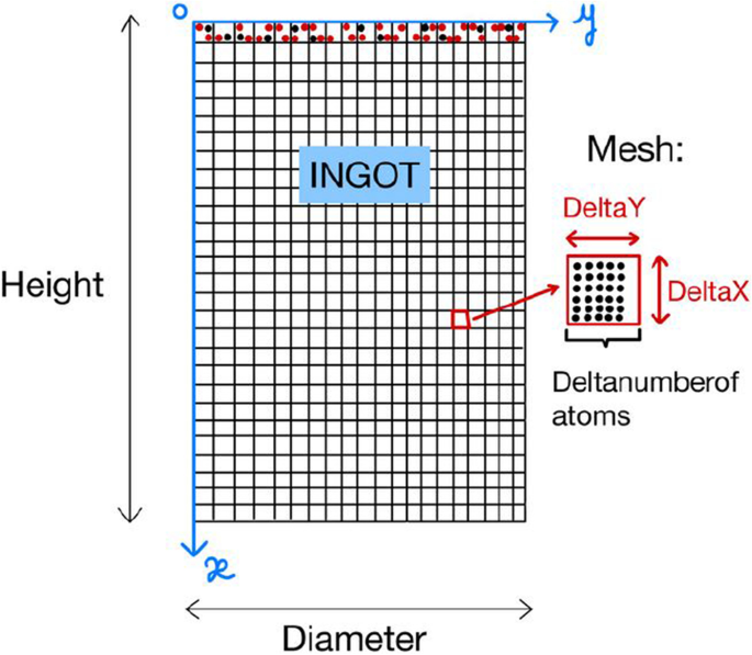

  

  Ingot representation in 2D

In addition to the user-defined arguments, the temperature distribution calculated and shown in Fig. 5 is also used by the model to establish the vapour pressure and evaporation rate on each of the constituent sub-species of the mesh. Optimisation is achieved when the modelled evaporation rate of the ingot matches that measured experimentally. This allows evaporation rates for the sub-component oxides to be determined, matched to the evaporation rates measured for the different ingot composition.

Following this optimisation Fixed values for the time and mesh size parameters are used when undertaking the simulations presented in this paper (Table 2) This enables comparison of the evaporation rates of different oxides and ease of evaporation of ingots of mixed oxide compositions.

Table 2 Value of parameters selected for the computational models

The pseudo-code of the computer model is available in reference [21]. The pseudo-code provides detail of the code and also the mathematical and analytical model.

2.2.1 2D model

Given the radial symmetry of the ceramic ingots, a programme simulating the evaporation in 2D was first created to gauge the computational cost of the evaporation model, before extending the model to 3D.

Before programming the evaporation itself, the ingot is modelled (Fig. 8). Six matrices in the programme represent the six sub-oxides possible within an ingot. Each matrix keeps track of the number of molecules in an element of the ingot deltaX*deltaY, considering the density and molar mass of each oxide and the oxide fraction out of the total composition. Consequently, the number of molecules in a mesh element is different for each of the 6 ceramic sub-oxides.

Using the computed value of the vapour pressure for each element and considering the thermal profile of the ingot surface (Fig. 6), the mass flow rate in kg/(cm²s) is calculated. Because the ingot elements have been defined based on the number of molecules they contain and not their mass, the mass flow rate is converted into molecules/(cm²s). The output produced by the model is the number of molecules that evaporate from each mesh element in the evaporation time, which is subtracted from the number in the original matrices.

A ‘while’ loop persists until the evaporation time has been reached. Once in the loop, the programme scans the top of the ingot for each element and calculates the number of molecules that evaporate as shown in Fig. 9. If an element of the mesh is empty, the programme automatically evaporates molecules in the element immediately below the empty element.

Fig. 9

Evaporation of molecules from the topmost element

2.2.2 3D model

The working principle of the 3D programme is the same as that for the 2D. The most significant difference is that the ingot is represented in 3D and we calculate the height of the target.

The variables are the same as 2D but adapted to 3D. Each sub-oxide in the ingot is represented by a ‘targetmatrix’ with a dimension MxM. The topmost elements of the ingot are represented by a rectangular matrix. A circle is defined using a function defined in MATLAB that assigns a value of 1 to all elements in the ‘targetmatrix’ within a circle, with the remaining elements being assigned a value of 0. Once the circle is created, all the elements with a value of 1 are replaced with the corresponding number of molecules. Schematic diagrams of ‘targetmatrix’ and the ingot are represented in Fig. 10.

Fig. 10

‘targetmatrix’ and the ingot representation in 3D

Once all variables are defined, evaporation starts in a loop iterating over evaporation time. In 3D, ‘targetmatrices’ keep track of the number of molecules left in each of the elements of the ingot surface. ‘Targetmatrixheight’ is defined for each oxide and represents the height of the target during the evaporation. The initial condition of ‘Targetmatrixheight’ is shown in Fig. 11, with the circle representing the ingot full, with a 16 cm height. During the evaporation, molecules from each sub-oxide are removed from the corresponding ‘targetmatrix’; this follows the temperature distribution from Fig. 5C. When a value of the targetmatrix becomes 0, it means that the corresponding element is empty and the following molecules to evaporate are deeper in the ingot. The corresponding value is updated in ‘Targetmatrixheight’ and the ‘targetmatrix’ is filled again to represent the next molecules evaporating. As shown in Fig. 11, the height is decreasing at the centre due to evaporation of molecules, as it is the hottest part of the ingot.

Fig. 11

‘Targetmatrixheight’ definition in 3D

2.2.3 Local composition activated model

In the 2D and the 3D programmes, we assume that the evaporation of molecules from one sub-oxide is independent from the evaporation of the others; thus some sub-oxides are evaporating faster than others. In practice, when a sub-oxide is evaporating faster, its concentration in the melt pool decreases. If its concentration decreases, fewer molecules will evaporate until the concentration increases again.

The 2D programme has been modified to consider this effect. For every iteration, the melt pool composition is re-calculated. If the concentration of one sub-oxide is higher than others, its evaporation rate is multiplied by $1+J\bullet {X}_{oxide}$, where ${X}_{oxide}$ is the mass fraction of the oxide in the melt pool and J an adjustment parameter equal to 1.7. The origin and determination of J are presented in the discussion. On the other hand, if an oxide has a lower concentration, its evaporation rate is multiplied by ${X}_{oxide}$ to decrease the evaporation speed. It locally activates the evaporation of species evaporating slowly and the model is called local composition activated (LCA).

3 Results

3.1 Demonstration of model results

The three models (2D, 3D and LCA) with parameters from Table 2 have been used to simulate the evaporation behaviour of an ingot of composition: 90 wt% ZrO₂, 7 wt% Y₂O₃, 3 wt% Er₂O₃. Table 3 illustrates the results of the three models segregated by sub-oxide. For each model, a graphical representation of the matrices is shown. The blue parts of the 2D and LCA graphs corresponding to empty areas where all molecules have evaporated, while the yellow areas are full of molecules; for the 3D graphs, the lack of molecules is represented by transparent volumes, yellow volumes represent areas full of molecules, and the external edge of the ingot is blue (cropped in some sections due to the selected graph boundaries).

Table 3 Visual representation of results’ matrices for 2D, 3D and LCA after 1,000 s of evaporation. The blue areas in the 2D graphs are empty of molecules, as are the transparent areas in 3D graphs, whereas yellow areas contain at least to some oxide molecules

The combination of graphs in Table 3 allows to calculate the mass evaporated, the evaporation rate, and to understand the differences between each sub-oxide. The usefulness of models 2D and 3D relies on the ability to compare the constituent’s evaporation speeds. Both models are in agreement, presenting the same amount of evaporated ingot for all sub-oxides except for a 2 mm difference that is an artefact of the pixel (DeltaX) size. These models reveal that yttria evaporates ~ 2.5 times faster than zirconia, whereas erbia evaporates at about half the rate of zirconia. The evaporation takes place preferentially in the central area, leaving a solid ring that surrounds the melt; this is a consequence of the lower temperature of the outer ring as calculated in Fig. 5 and Fig. 6. However, it is clear that a real ingot won’t show such large discrepancies on the evaporation of its different constituents. To calculate a realistic ingot evaporation depth, the LCA model is used. This model harmonises the evaporation of all the different constituents and results in a final ingot evaporation depth of 18 mm, which is clearly dominated by the larger fraction of zirconia (the 18-mm depth value is very similar to the zirconia depth values of models 2D and 3D). The evaporation rate is therefore ~ 1 mm/s, similar to the experimental evaporation rate observed using Cranfield University’s EB-PVD coating system on erbia-doped 7YSZ at 20 kW.

3.2 Oxide evaporation speed comparison

This section is exclusively concerned with the evaporation speed of different oxides. The 2D model (with Table 2 parameters) was applied to oxides ZrO₂, Y₂O₃, Gd₂O₃, Er₂O₃, La₂O₃, and Yb₂O₃ without any specific ingot composition in mind, so all oxide fractions were set to 100 wt%. The results of the evaporation modelling, summarised in Table 4, show that it has an evaporation rate an order of magnitude faster than the rest of oxides. Yttria and gadolinia have a similar evaporation rate that is between 2 and 3 times larger than those for zirconia, erbia and ytterbia, which display an almost identical value that is about 10 times slower than lanthana. These results broadly agree with reported difficulties for lanthana-doped zirconia evaporation and are compared with the literature in the discussion section. It is worth noting that the evaporation speeds are affected by the oxide composition fraction introduced in the model; an example of this is the difference between the erbia rates presented in Table 3 and Table 4.

Table 4 Results for the oxide evaporation rate simulation

3.3 Evaporation of typical TBC ingot compositions

The three computational models have been applied to typical commercial TBC ingots, again using the parameters in Table 2. The more extended TBC compositions are based on yttria-stabilised zirconia (YSZ). Lately, rare-earth zirconates have attracted attention as candidate materials for advanced TBC systems [19, 22]. Gd₂Zr₂O₇, gadolinium zirconate (GZO), is an increasingly popular composition.

Therefore, two ingots representing the two different chemistries have been simulated. The first ingot (7YSZ) is composed of 7 wt% yttria and 93 wt% zirconia. The second ingot (GZO) is composed of 40.5 wt% ZrO₂ and 59.5 wt% Gd₂O₃, which corresponds to stoichiometric Gd₂Zr₂O₇. The results, summarised in Table 5, show a similar behaviour of the two ingot compositions. All discrepancies between 2 and 3D models, and between the different constituent oxides of the ingots for in local composition activated model are in the range of one DeltaX and therefore negligible at the scale of this model. For both ingots, the presence of yttria or gadolinia accelerates the natural evaporation rate of zirconia. The GZO ingot evaporates slightly faster than the 7YSZ, which matches experimental experience for evaporation under the same electron-beam power. In practice, 7YSZ is often evaporated at slightly larger powers due to its higher melting point, which increases its evaporation rate.

Table 5 Evaporation rates for sub-oxides in 7YSZ and GZO given by different models

The calculation of evaporation rate in terms of length of ingot per unit of time is useful to be directly compared to and applied in experimental evaporation. However, the models also allow to calculate the total material evaporated. The number of molecules evaporated can then be divided per unit of time and unit of matrix (voxel) to obtain an evaporation rate which is more relevant to the total material evaporated; this rate is not affected by the ring of unmolten material, which can be uneven on deep evaporations as seen in Table 3. Table 6 contains the result of this evaporation rate for GZO and compares it to the respective vapour pressures of the constituent oxides. It is noticeable that, although the trends are maintained, the ratio of the evaporation rates is not identical to the vapour pressures, which is considered further in the discussion section.

Table 6 Evaporation rate and vapour pressure comparison

3.4 Evaporation of advanced TBC ingot compositions

The model has also been applied to the evaporation of novel rare-earth zirconates, which have been proposed as candidates for advanced TBC systems. The evaporation of rare-earth zirconates can be challenging due to the different vapour pressures of the different constituent oxides, and our models can help in designing strategies to overcome these difficulties.

One strategy consists in using oxides with similar vapour pressures and evaporation rates. The results from Table 4 indicate that Ytterbia has a very similar evaporation rate to zirconia, and thus in the first simulation Yb₂O₃ will replace Gd₂O₃ from the previous section to generate Yb₂Zr₂O₇. The models, again following Table 2 parameters, applied to an ingot composed of 38.4 wt% ZrO₂ and 61.6 wt% Yb₂O₃ confirm that the expected evaporation rates are very similar (Table 7).

Table 7 Evaporation rates for an ytterbium zirconate ingot

Another strategy consists in adding small quantities of a third oxide to moderate the evaporation of high vapour pressure rare-earth oxides. This overcomes the limitations of the first strategy that constrains the diversity of oxides that are usable. An example of this strategy has been deployed with lanthanum zirconate (LZO—La₂Zr₂O₇). One of the challenges in the evaporation of LZO is the preferential evaporation of La₂O₃, which has an evaporation rate an order of magnitude larger than ZrO₂ (Table 4). This gives raise to fluctuating evaporation and compositional segregation in the coatings produced [23], which can be moderated by the addition of other oxides, such as Y₂O₃. We explored the possibility of slowing evaporation by adding 1.5 to 9 wt% of Y₂O₃ to the ingot composition and compared it to pure La₂Zr₂O₇ in a series of LCA simulations detailed in Table 8, using parameters from Table 2. The results revealed that even small additions of yttria have a powerful effect on the sub-oxide evaporation rates, reducing them by 50%. However, the results also suggest that the quantity of yttria employed is not relevant, as long as at least 1.5 wt% is present. In the literature, usually a 3 wt% of yttria is employed with successful moderating effects [22, 23].

Table 8 Ingot composition of different (La,Y)₂Zr₂O₇ ingots with their respective sub-oxides evaporation rates

4 Discussion

4.1 Temperature of the ingot

Calculating the ingot temperature is challenging because obtaining precise temperature measurements of the ingot surface is difficult within a vacuum chamber. An initial estimation can be made by comparing the surface colour to the black body radiation spectrum. The ingot has a yellow colour that corresponds to a surface temperature of around 4000 K.

Iterative Abacus simulations were performed using the known input electron-beam (EB) energy, typically 20 kW. In a scenario where all energy is absorbed by the ingot and the only heat transfer mode is through conduction to the water-cooled hearth, the surface temperature should reach 22,670 K. This result highlights the extent of energy dissipation by radiation in the chamber, conduction in the ingot and evaporation of the material. An iterative process was conducted by altering the fraction of energy dissipated by radiation and calculating the resulting ingot surface temperature. The process was stopped when the surface temperature of the ingot reached 4,100 K, similar to the estimated temperature of the target, which suggested that ~ 78% of the energy coming from the electron beam is dissipated radiatively. This corresponds well with experimental experience, where sample temperature increases sharply after evaporation begins.

Related to this result, Ohba and Shibata [24] studied the temperature profile on a liquid metal surface during EB-evaporation. They focused an EB with different powers on a copper ingot and measured the surface temperature using a charge coupled device (CCD) camera. By applying their calculated regression curve between EB power and surface temperature, and adjusting for the differences in ingot size employed by Ohba and Shibata (50 mm in diameter) and ours (40 mm), the resulting estimated temperature for 7YSZ is 3,289 K. This result somewhat differs from the 4,100 K calculated by iterative simulations, although it is of the right order of magnitude. There are two main factors that can account for the difference: extrapolation and material differences. The first factor considers that Ohba and Shibata’s regression curve only extended to an EB power of 4.5 kW compared to the 20 kW of the simulation; therefore, the curve is extrapolated far beyond their experimental data points. The second factor is that their experiments considered metal copper in a crucible, as opposed to ceramic ingots; the higher conductivity of copper might account for a lower surface temperature (as heat can be more easily transmitted to the hearth).

Moreover, the percentage of energy dissipated could be overestimated due to the assumptions made in the model. The water cooling is modelled with a constant temperature on the ingot sides. This differs from the reality because the water cooling is an outgoing heat flux decreasing the ingot temperature. Modifying this parameter could give a better approximation of the energy dissipated.

There are other limitations as well. The vapour plume is not made of Zr atoms only, but a mix of ZrO₂, ZrO and O₂ [25], as ZrO₂ can lose an oxygen atom during evaporation. To achieve a stoichiometric mix, the chamber is filled with oxygen gas, which adds another layer of complexity not considered here. The melt pool is not in a metallic state, but it is reasonable to take the conductivity of Zr for the melt pool. This conductivity is multiplied by 100 to consider the effect of convection in the liquid as a broad approximation, as no reliable value could be found in the literature for convection and convective stirring in a melt pool.

4.2 Oxide comparisons

Evaporation speed varies between oxides; for example, Y₂O₃ evaporates twice as fast as ZrO₂. It is important to understand this phenomenon because evaporation speed differences in the ingot could lead to compositional differences in the coating [8, 19, 22, 23]. As explained in the analytical model, evaporation speed mainly depends on two parameters: the vapour pressure and the mass flow rate. If a species has a greater vapour pressure and mass flow rate, it will evaporate faster compared to another and ultimately lead to the depletion of the fastest evaporating oxide.

In 1989, Jacobson [26] compared the vapour pressure of rare-earth oxides. The vapour pressures at 2,500 K are shown in Table 9 using yttria as a reference. Table 9 also contains the relative evaporation rates from Table 4 also referenced to yttria to be comparable to the first column.

Table 9 Relative vapour pressure and evaporation rate comparison between 5 rare-earth oxides from source [26] and Table 4, respectively

The vapour pressure of La₂O₃ is 65 times higher than the vapour pressure of Y₂O₃. We also observed a large difference in Sect. 3.2, with the evaporation speed comparison being 2.88 mm/min for Y₂O₃ and 14.88 mm/min for La₂O₃ (~ 5 × higher). The model predicts La₂O₃ to be the fastest evaporating oxide, as expected from its higher vapour pressure, although the differential ratio is smaller than one might expect based on the vapour pressure difference. The same is observed with the rest of the oxides; there are differences between the partial pressures and the evaporation rates calculated from the models. These differences arise from the model accounting for more aspects apart from the vapour pressure, such as molecular mass and density which influence the evaporation rate. This reflects the advantage of using the model when developing new evaporation materials, as opposed to only relying on relative vapour pressures.

The moderating effect of Y₂O₃ on the evaporation of LZO appears to be insensitive to the content of Y₂O₃, once some critical content is reached (around 1.5 wt%, maybe less), so in this study for the composition range 1.5–9 wt% Y₂O₃, the evaporation rate no longer depended on yttria content. This suggest that a tolerant processing window exists for the evaporation of LZO doped with Y₂O₃, potentially enabling compositional tuning of LZO to produce TBCs with desired properties. Even if a species has a higher vapour pressure, it can evaporate slowly compared to other oxides. This is because the evaporation rate also depends on other parameters such as the oxide mass and the temperature distribution.

This model, conveniently modified, could also be useful in other multi-element evaporation applications, such as metal alloys. For instance, the work of Ali et al. [27] describes how different EB powers produce different evaporation on different alloying elements in stainless steel EB-PVD deposition, which could potentially be modelled and predicted by an adapted version of the model presented in this paper.

4.3 Evaporation rate ratio comparison

Another way to validate the MATLAB simulation is to use the evaporation rate ratio formula. In 2011, Kember [8] studied the effect of differences in vapour pressure between two species. He found that the evaporation rate ratio between two species is linked to the composition in the melt pool, the vapour pressure and the molecular weight of species following (evaporation rate ratio formula for two species).[8].

$$\frac{{\alpha }_{A}}{{\alpha }_{B}}= \frac{{X}_{A}{P}_{A}{M}_{A}^{1/2}}{{X}_{B}{P}_{B}{M}_{B}^{1/2}}$$

with ${\alpha }_{A}$ the evaporation rate ratio of A, ${X}_{A}$ the mole fraction of A in the melt pool, ${P}_{A}$ the vapour pressure of A and ${M}_{A}$ the molecule weight of A. This formula can be applied to the results of GZO evaporation from Table 6. The ratio between evaporation rates of ZrO₂ and Gd₂O₃ is 1.46, and the ratio for the right part of the equation is 1.9. Both values are of the same order of magnitude, demonstrating that the results obtained from the MATLAB simulation are broadly in agreement with the results from the literature. One of the objectives is to produce data for the evaporation that represents reality. It is the case with the evaporation of GZO.

Moreover, the evaporation rate ratio formula can be generalised for more than two species with (evaporation rate ratio formula for 3 species A, B and C):

$$\frac{{\boldsymbol{\alpha }}_{{\varvec{A}}}}{{{\boldsymbol{\alpha }}_{{\varvec{A}}}+\boldsymbol{\alpha }}_{{\varvec{B}}}+{\boldsymbol{\alpha }}_{{\varvec{C}}}}=\frac{{{\varvec{X}}}_{{\varvec{A}}}{{\varvec{P}}}_{{\varvec{A}}}{{\varvec{M}}}_{{\varvec{A}}}^{1/2}}{{{{\varvec{X}}}_{{\varvec{A}}}{{\varvec{P}}}_{{\varvec{A}}}{{\varvec{M}}}_{{\varvec{A}}}^{1/2}+{\varvec{X}}}_{{\varvec{B}}}{{\varvec{P}}}_{{\varvec{B}}}{{\varvec{M}}}_{{\varvec{B}}}^{1/2}+{{\varvec{X}}}_{{\varvec{C}}}{{\varvec{P}}}_{{\varvec{C}}}{{\varvec{M}}}_{{\varvec{C}}}^{1/2}}$$

Taking an ingot with 89 wt% ZrO₂, 7 wt% Y₂O₃ and 4 wt% Er₂O₃, the simulation gives the results shown in Table 10. When applied to, the left part is equal to 0.89, and the right part is equal to 0.90. There is, again, good agreement that demonstrates that the model also follows the evaporation rate ratio formula for more than two species.

Table 10 Evaporation rate and vapour pressure of ZrO₂, Y₂O₃ and Er₂O₃

4.4 Determination of the activation parameter in the local composition activated evaporation

Modelling the evaporation of an ingot with multiple constituent oxides is complex. As mentioned before, models 2D and 3D were designed to compare the different evaporation rates of the different oxides and determine if preferential evaporation was likely to occur. However, the main limitation of those models is that they cannot calculate the evaporation rate of the aggregate oxides, i.e. the ‘real’ evaporation rate of the whole ingot. Therefore, these models cannot account for the moderating effect of certain oxides, nor can they be applied for the estimation of experimental evaporation rates. This is because models 2D and 3D consider evaporation of each constituent oxide in isolation, only considering the oxide’s properties and weight fraction. In reality, when preferential evaporation of an oxide takes place, the melt pool is left with a composition richer in the other sub-oxides and there is momentarily less matter to absorb the same EB energy. This results in a period where the evaporation rate of the other oxides is increased, until more of the preferentially evaporated oxide melts, fuses into the melt pool and is then evaporated. The cycle repeats itself, and it gives rise to the banding across coating thickness sometimes reported in the literature [8, 19, 22, 23].

The LCA model attempts to recreate this cyclic mechanism and estimates the evaporation rate of the aggregate of all the sub-oxides. To this end, the model introduces a coefficient J that represents the degree of enrichment of the other sub-oxides once their concentration in a unit cell is much larger than that of the preferentially evaporating oxide. Once the concentration threshold is surpassed, the evaporation rate of the predominant oxide is multiplied by $1+J\bullet {X}_{oxide}$, with ${X}_{oxide}$ the oxide composition in the melt pool. Coefficient J is not directly relatable to any physical mechanism but rather attempts to simulate the faster evaporation of species enriched in the melt pool; therefore, its value had to be iterated and its effect compared with experimental evaporation rates. The iterative simulation process was done over an evaporation time of 1,800 s, with a mesh size DeltaX = 2 mm and DeltaY = 1 mm, simulating an ingot of stoichiometric Gd₂Zr₂O₇ (so 40.5 wt% of ZrO₂ and 59.5 wt% of Gd₂O₃). The value of J was increased from 1.4 to 2, and evaporation speeds of both oxides were compared to evaporation speed from the Cranfield university coater of Gd₂Zr₂O₇ under 20 kW of EB power. The results, summarised in Table 11, show that the value of J that more closely replicates the experimental results is 1.7. Further detail of the simulation can be found in Fig. 12, which contains the ratio of evaporation rates of lanthana and zirconia of the first 1000 s. The absolute evaporation rates of the two oxides that have been used to calculate the ratio of the previous graph are presented in Fig. 13.

Table 11 Evaporation rates for oxides in GZO for different values of J compared to experimental results

Fig. 12

Temporal evolution of the ratio between evaporation rates of lanthana and zirconia calculated using different values of J by LCA model for the first 1000 s

Fig. 13

Temporal evolution of the evaporation rates of two constituent oxides (lanthana and zirconia) calculated using J = 1.7 by LCA model for the first 1000 s

This method provides reasonable results for the adjustment of the evaporation rates of the different oxides based on the composition variation in the melt pool. It successfully replicates the cyclic changes in evaporation rates of different oxides observed in literature, as illustrated in Figs. 12 and  13. The graphs also indicate that the cycle frequency increases with the value of J. Experimental observation of coating banding could be compared to the simulated cycles to further refine the value of J. Some degree of stabilisation is achieved within the time frame of the graph. More importantly, it also predicts the evaporation rate of the aggregate oxide. Despite these good results, other methods could be considered to overcome some of the limitations of the model. One of the possibilities is to create an equilibrium condition in the melt pool with the evaporation rate ratio formula. Some preliminary work was initiated, but it did not give consistent results and further work is required. Further refinements could be also account for heat dissipation through radiation and advection.

5 Conclusions

This paper presents three computational models to simulate ingot evaporation during electron-beam physical vapour (EB-PVD) deposition. The models aid in the development of new thermal barrier coatings, especially those of rare-earth zirconates, as they allow for rapid screening of different ingot compositions to evaluate the effect of preferential evaporation of the constituent oxides, which if unchecked can lead to compositional segregation within the deposited coating, and to characterise the aggregate evaporation rate. Modifications of the model could be applied to predict the evaporation of other multiple-element materials and alloys.

The computational models simulate key steps of a larger analytical model aimed as digital twin of the EB-PVD process: that is proposed to characterise the whole evaporation process. For this, some simplifications and assumptions have been made, such as the temperature distribution on the ingot surface and the amount of energy dissipated by radiation and conduction (78%). Those simplifications and assumptions have been checked against data available in the literature and against thermodynamic simulations.

The models called 2D and 3D have been developed to evaluate the difference in evaporation rates of the constituent sub-oxides of an ingot. The model called ‘local composition activated’ (LCA) is a refinement of model 2D that can be used to calculate the aggregate evaporation rate of an ingot with multiple constituent oxides. LCA introduces an activation coefficient that successfully reproduces the cyclic changes in evaporation rates that lead to compositional segregation (banding) of the coating. The models have been validated using the evaporation rate ratio formula, results from experimental evaporation in Cranfield University coaters and vapour pressure calculations from the literature.

Results from such simulations have been exploited for a better understanding of the evaporation process for complex oxide systems. It has shown that some species are evaporating faster, due mainly to the vapour pressure effect on their evaporation rate, but not directly to their partial vapour pressure. The model also showed the influence of the melt pool composition on the evaporation rate. Both of these factors are important, and observations are consistent with experimental experiences.

While progress has been made to better understand and model complex oxide evaporation, further simulation work is still needed to fully characterise the EB-PVD process and, thus, propose a complete simulation model. The following steps include the modelling of vapour fragments, modelling of displacements of these molecular parts within the chamber, their recombination, deposition and growth of the coating on the substrate, therefore, linking evaporation, transport and deposition. Regarding evaporation, further refinement could include the addition of various sub-oxides during evaporation, the introduction of variable porosity within the ingot structure and expanding available experimental data and heat transfer mechanisms affecting the surface temperature distribution achieved within the melt pool.

References

K.G. Kyprianidis, Future aero engine designs: an evolving vision. Ad. Gas Turbine. Tech. (2011). https://doi.org/10.5772/19689
M. Kawamura, Y. Matsuzaki, H. Hino, S. Okazaki, Evaluation of graded thermal barrier coating for gas turbine engine. Functionally Graded Materials 1996. (1997), pp. 413–418. https://doi.org/10.1016/B978-044482548-3/50068-8
H. Xu, H. Guo, S. Gong, 16- Thermal barrier coatings. Developments in High-Temperature Corrosion and Protection of Materials. (2008), pp. 476–491. https://doi.org/10.1533/9781845694258.2.476
D.L. Poerschke, J.S. Van Sluytman, K.B. Wong, C.G. Levi, Thermochemical compatibility of ytterbia-(hafnia/silica) multilayers for environmental barrier coatings. Acta. Materialia. 61(18), 6743–6755 (2013). https://doi.org/10.1016/j.actamat.2013.07.047 (Acta Materialia Inc)
DM. Mattox, Handbook of Physical Vapor Deposition (PVD) Processing. Noyes publications. (1998), pp. 31–33. https://doi.org/10.1515/9783110971828.1
G. Faraji, H. Torabzadeh Kashi, HS. Kim, Severe plastic deformation - methods, processing and properties. (2018), pp. 1–17. https://doi.org/10.1016/C2016-0-05256-7
D. Zhang, 1 - Thermal barrier coatings prepared by electron beam physical vapor deposition (EB–PVD). Thermal Barrier Coatings. (2011), pp. 3–48. https://doi.org/10.1533/9780857090829.1.3
T. Kember, Compositional variations in vapor deposited samarium zirconate coatings. PhD Thesis, University of Virginia (2011).
JR. Nicholls, KJ. Lawson, A. Johnstone, DS. Rickerby, Methods to reduce the thermal conductivity of EB-PVD TBCs. Surface and Coatings Technology. 151–152, 383–391 (2002). https://doi.org/10.1016/S0257-8972(01)01651-6
G. Yang, CY. Zhao, Infrared radiative properties of EB-PVD thermal barrier coatings. Int. J. Heat. Mass. Transfer. 94, 199–210 (2016). https://doi.org/10.1016/j.ijheatmasstransfer.2015.11.063
I. Fuke, V. Prabhu, S. Baek, Computational model for predicting coating thickness in electron beam physical vapor deposition. J. Manuf. Process. 7(2), 140–152 (2005). https://doi.org/10.1016/S1526-6125(05)70091-8
S. Baek, V. Prabhu, Finite element model for unified EB-PVD machine dynamics. Surf. Eng. 23(6), 453–463 (2007). https://doi.org/10.1179/174329407X239225
S. Baek, V. Prabhu, Simulation model for an EB-PVD coating structure using the level set method. J. Manuf. Process. 11(1), 1–7 (2009). https://doi.org/10.1016/j.jmapro.2009.05.001
R.G. Wellman, M.J. Deakin, J.R. Nicholls, The effect of TBC morphology and aging on the erosion rate of EB-PVD TBCs. Tribol. Int. 38(9 SPEC. ISS.), 798–804 (2005). https://doi.org/10.1016/j.triboint.2005.02.008
A. Waddie, P. Schemmel, C. Chalk, L. Isern, J. Nicholls, A. Moore, Terahertz optical thickness and birefringence measurement for thermal barrier coating defect location. Opt. Express 28(21), 31535–31552 (2020). https://doi.org/10.1364/OE.398532
G. Boissonnet, F. Pedraza, C. Chalk, J.R. Nicholls, G. Bonnet, Thermal insulation of YSZ and Erbia-doped yttria-stabilised zirconia EB-PVD thermal barrier coating systems after CMAS attack. Materials. 13(19), 1–16 (2020). https://doi.org/10.3390/ma13194382
G. Boissonnet, C. Chalk, J.R. Nicholls, G. Bonnet, F. Pedraza, Phase stability and thermal insulation of YSZ and erbia-yttria co-doped zirconia EB-PVD thermal barrier coating systems. Surface and Coatings Technology. 389, 125566 (2020). https://doi.org/10.1016/j.surfcoat.2020.125566
Granta Design Ltd. CES Edupack software. Cambridge (2013).
U. Schulz, B. Saruhan, K. Fritscher, C. Leyens, Review on advanced EB-PVD ceramic topcoats for TBC applications. App. Ceram. Technol. 1(4), 302–315 (2004). https://doi.org/10.1111/j.1744-7402.2004.tb00182.x
R. Schmidt, M. Parlak, A.W. Brinkman, Control of the thickness distribution of evaporated functional electroceramic NTC thermistor thin films. J. Mater. Process. Technol. 199(1), 412–416 (2008). https://doi.org/10.1016/j.jmatprotec.2007.08.014
J. Chevallier, L. Isern, K. Almandoz Forcen, C. Chalk, J.R. Nicholls, Pseudo-code EBPVD evaporation. (2021). https://doi.org/10.17862/cranfield.rd.14519943
J. Zhang, X. Guo, Y.G. Jung, L. Li, J. Knapp, Lanthanum zirconate based thermal barrier coatings: a review. Surf. Coat. Technol. 323, 18–29 (2017). https://doi.org/10.1016/j.surfcoat.2016.10.019
B. Saruhan, P. Francois, K. Fritscher, U. Schulz, EB-PVD processing of pyrochlore-structured La2Zr2O7-based TBCs. Surf. Coat. Technol. 182(2–3), 175–183 (2004). https://doi.org/10.1016/j.surfcoat.2003.08.068
H. Ohba, T. Shibata, Temperature profiles on liquid metal surface during electron beam evaporation. Jpn. J. Appl. Phys. 34(8 R), 4253–4257 (1995). https://doi.org/10.1143/JJAP.34.4253
M.M. Nakata, R.L. McKisson, B.D. Pollock, Vaporization of zirconium oxide. Atomics International (1961).
N. S. Jacobson, Thermodynamic properties of some metal oxide-zirconia systems. NASA Technical Memorandum (1989).
N. Ali, J.A. Teixeira, A. Addali, M. Saeed, F. Al-Zubi, A. Sedaghat et al., Deposition of stainless steel thin films: an electron beam physical vapour deposition approach. Materials. 12(4), 1–16 (2019). https://doi.org/10.3390/ma12040571
Acknowledgements
The authors would like to thank the invaluable contribution of Tony Gray, senior technical officer at Cranfield University, for his work and experience in EB-PVD deposition. The authors are also grateful to Dr Gyaneshwara Brewster, Dr Robert Jones and Mr Alan Johnstone, all coating specialists from Rolls-Royce Plc, for their helpful discussions.
Author information
Authors and Affiliations
Contributions
All authors contributed to formal analysis and investigation, methodology and manuscript review and editing. Original draft produced by J Chevallier and L Isern. Original figures produced by J Chevallier, L Isern and K Almandoz Forcen. Original computer model designed and coded by J Chevallier with input from the rest of the authors. Simulations executed by J Chevallier and K Almandoz Forcen.
Corresponding author
Ethics declarations
Conflict of interest
The authors declare no competing interests.
Rights and permissions
Open Access This article is licensed under a Creative Commons Attribution 4.0 International License, which permits use, sharing, adaptation, distribution and reproduction in any medium or format, as long as you give appropriate credit to the original author(s) and the source, provide a link to the Creative Commons licence, and indicate if changes were made. The images or other third party material in this article are included in the article's Creative Commons licence, unless indicated otherwise in a credit line to the material. If material is not included in the article's Creative Commons licence and your intended use is not permitted by statutory regulation or exceeds the permitted use, you will need to obtain permission directly from the copyright holder. To view a copy of this licence, visit http://creativecommons.org/licenses/by/4.0/.
About this article
Cite this article
Chevallier, J., Isern, L., Almandoz Forcen, K. et al. Modelling evaporation in electron-beam physical vapour deposition of thermal barrier coatings. emergent mater. 4, 1499–1513 (2021). https://doi.org/10.1007/s42247-021-00284-5
Received:
Accepted:
Published:
Issue Date:
DOI: https://doi.org/10.1007/s42247-021-00284-5