Critical Correlation of Predictors for an Efficient Risk Prediction Framework of ICU Patient Using Correlation and Transformation of MIMIC-III Dataset

Abstract

Various predictive frameworks have evolved over the last decade to facilitate the efficient diagnosis of critical diseases in the healthcare sector. Some have been commercialized, while others are still in the research and development stage. An effective early predictive principle must provide more accurate outcomes in complex clinical data and various challenging environments. The open-source database system medical information mart for intensive care (MIMIC) simplifies all of the attributes required in predictive analysis in this regard. This database contains clinical and non-clinical information on a patient’s stay at a healthcare facility, gathered during their duration of stay. Regardless of the number of focused research attempts employing the MIMIC III database, a simplified and cost-effective computational technique for developing the early analysis of critical problems has not yet been found. As a result, the proposed study provides a novel and cost-effective machine learning framework that evolves into a novel feature engineering methodology using the MIMIC III dataset. The core idea is to forecast the risk associated with a patient’s clinical outcome. The proposed study focused on the diagnosis and clinical procedures and found distinct variants of independent predictors from the MIMIC III database and ICD-9 code. The proposed logic is scripted in Python, and the outcomes of three common machine learning schemes, namely Artificial Neural Networks, K-Nearest Neighbors, and Logistic Regression, have been evaluated. Artificial Neural Networks outperform alternative machine learning techniques when accuracy is taken into account as the primary performance parameter over the MIMIC III dataset.

1 Introduction

The use of science in the healthcare industry has transformed the approach to understanding diseases, treatment, patient care, and hospital management planning. The joint science system with healthcare has emerged as a novel model, namely, the Prospective Health Care Model (PHCM). The PHCM is a probabilistic model to predict the possibilities of future medical conditions in advance so that - an optimal healthcare plan can be perceived from both the patient and the hospital management perspectives [19]. Irrespective of the sum of 1.5 trillion dollars per year expenditure for healthcare in the USA, approximately 40 million Americans lack ready access to health services [6]. A critical dimension of the healthcare system is balancing a cost burden to payers as individuals or insurers. The chosen research study is towards building a model of PHCM to determine the potential risk in advance based on the respective diagnosis-procedure applied to the intensive care unit patients. During critical health conditions, patients are admitted to intensive care units (ICUs) to treat various diagnoses. Such admission can either be into one specific ICU or in multiple ICUs to get diagonalized with the specific medical devices. Based on the diagnosis, the physician chooses a suitable set of procedures for the patient. In this process, the physician also needs to find the correlation between various types of clinical procedures and their anticipated healing outcomes. The retention of patients in the ICU is limited to the procedure level. One of the critical requirements from the hospital management perspective and patient’s well-being is predicting random readmission due to the risk of complexities after providing specific procedures and discharge [15]. Advanced healthcare data acquisition technologies acquire various formats of data from multiple dynamic sources over a timeline [3, 7, 20] and a distributed file system-oriented data-models support the intrinsic characteristics like heterogeneity, uncertainty, and high dimensionality of these data [5, 9]. There is a growing trend in data processing and artificial intelligence to build reporting and billing applications in the healthcare industry using these data [2, 26]. Concurrently, research interests are growing exponentially to build efficient prediction models to provide an automatic decision support system to be beneficial for both patients and caretaking personnel [23, 24, 29]. However, the research community faces a seamless synchronization between learning tasks and data experience without a flexible and easy-to-use collaboration between standard data access mechanism to the repository and standard processing algorithms [25]. A joint initiative of (i) MIT Clinical Inferencing Group, (ii) Philips CareVue system Philips HealthCare and, (iii) Beth Israel Deaconess Medical Centre, as in Fig. 1, has established a project under NIBIB to collect comprehensive data of intensive care unit (ICU) and produces as MIMIC-dataset [13].

Fig. 1

Comprehension of data within the MIMIC dataset by the National Institute of Biomedical Imaging and Bioengineering (NIBIB)

MIMIC provides: (i) Clinical Data: {ICU-information, hospital-archives}, (ii) physiological Data: {vital sign: $\rightarrow$ waveforms, time series} and, (iii) Death Data: {Death-Files}. The following are the significant information about this dataset:

• It records the patient's ICU admission till patient discharge.

• The acquired data are continuous to the related events.

• It includes demographic, administrative, physiologic, medication, testlab, discharge summaries.

The authorities keep updating the versions of MIMIC data and produce it from time to time, open to the research community after a compulsory formality of an examination as a pre-requisite. The first significant update to the MIMIC dataset appears from 2008 to 2012 as MIMIC-II and subsequently MIMIC-III with 60,000 ICU admissions. Table 10 describes all the dataset files with explicit information of its size on disk, number of columns, number of rows, and associated remarks that provide first-hand information for the data scientist to have an exploratory snapshot about the MIMIC-III dataset [16]. This paper proposes a prospective health care model-based framework on the MIMIC-III dataset for predicting the probability of readmission of the patient based on the risk associated with a particular procedure applied before discharging the patient from the hospital. The major obstacle to building an effective predictive system on the MIMIC-III dataset is complex feature engineering challenges [21]. The availability of large datasets like MIMIC-III provides abundant opportunities to build risk models, but it is under-exploited [12]. Therefore, an appropriate and effective feature engineering approach is required to create a feature vector for designing reliable predictive models using machine learning-based AI systems

The main highlights of this research paper are the challenges of obtaining the global feature vector and identifying the dependencies of variables with potential correlation on the vast and varied MIMIC-III dataset for designing an ML-based predictive model to visualize the insights of the hidden knowledge for a specific patient with their procedure and associated risk. The explicit benefit of feature engineering overcomes the limitations of the labour-intensive and naïve extraction process, which usually overlooks outliers’ dependencies and irregularities [18]. Therefore, practical feature engineering builds a base for more effective predictive models with reduced computational complexities. Section 2 highlights some contributions towards building predictive models and their dependencies on the feature engineering process; Sect. 3 highlights the research problem, while Sect. 4 describes the analytical modeling of feature engineering and design constructs of a learning model for risk prediction correlated with the applied procedure. Section 5 illustrates the result analysis followed by the conclusion in Sect. 6.

2 Existing Predictive Models Using the MIMIC III Dataset

At present, there are various research attempts to develop a predictive model using the MIMIC-III dataset. According to a recent study conducted by Moor et al. [14], machine learning contributes to developing a predictive model associated with sepsis. The study concludes that there are open-end challenges associated with sepsis’s predictive performance, which impedes benchmarking. Another recent work, by El-Rashidy et al. [4] indicated that; using a stacking ensemble approach where a predictive model could be developed to predict mortality rates. Johnson et al. [10] took a similar approach in their research, using the MIMIC dataset to predict mortality. Zeng et al. [28] recently published a study establishing the connection between a hospital visit and medical codes to develop a predictive model for the upcoming diseases. Ghassemi et al. [8] introduced a new predictive model in which auto-regression models are employed for unsupervised training. The study states that the predictive performance improves when original vital signs are paired with demographics and learned from. Many other studies have documented the adoption of such demographics. Veith and Steele [22] used machine learning to develop a predictive model for analyzing mortality rates in their study. Adoption of the MIMIC III dataset has also been analyzed by Shi et al. [17]where a predictive scheme for diagnosis is discussed. The study emphasizes both disease diagnosis and mortality prediction at the same time. The research uses a multi-source tasking strategy. The work carried out by Alshwaheen et al. [1] utilized recurrent neural networks. The outcome of the study revealed that the model is capable of reducing the dependency of the observation window significantly. Yu et al.’s [27] publication used a recurrent neural network for mortality risk prediction. The following section discusses the research problems associated with the existing approaches.

3 Research Problems

Here is the identification of the research problems after reviewing existing schemes:

• It has been observed that there are approximately less than 20 journals associated with the MIMIC III dataset implementation published in the recent five years in IEEE Xplore. A similar trend has also been witnessed for other publications. These studies have examined a variety of issues that can arise while diagnosing a specific illness condition. As MIMIC III is related to critical care information, it is essential to carry out more investigation. The complexities of the MIMIC-III dataset are vastly different compared to another standard healthcare dataset.

• Although Machine Learning is one of the dominant forms of the analytical and predictive mechanism used in medical datasets, the ranges of the study implementation in this regard are quite a few. Even considering that deep learning and other related predictive operation is significantly known, applying them will further introduce more complexities in implementation. It is because of the trade-off between explainability and performance [11] Although deep learning approaches suit well for more extensive data (i.e., MIMIC-III), they will still introduce a dependability issue when it comes to accuracy performance. The model will offer increased accuracy only with the condition of the availability of a larger trained dataset. Apart from this, such models too cannot comprehend outcomes based on sophisticated training only, and they will always depend on the selection of specific classifiers. Moreover, choosing an appropriate deep learning model itself is a challenging task regarding the accuracy of the critical care dataset.

• Feature engineering is another potential trade-off that has been noticed. Despite the abundance of existing feature engineering approaches, deep learning approaches are preferred since they have fewer dependencies. However, because of the challenges with deep learning indicated in the previous paragraph, MIMIC-III will need to evolve with a novel feature extraction approach. Apart from deep learning, other forms of machine learning approaches also do offer feature extraction processes. However, a cost-effective feature engineering process is still not reported in existing studies considering the MIMIC-III dataset.

Hence, looking at the points mentioned above as a research challenge, the proposed system aims to address these concerns computationally and cost-effectively. The following section discusses the solution introduced by the proposed feature engineering model.

4 Feature Engineering Analytical Model

The ICD-9-CM codes are the standard to describe the coding in the healthcare sector for different symptoms, diseases, injuries, and conditions. Table set: 1, 5, 12, 14, 21, 24, 25 MIMIC-III clinical dataset file descriptions (refer Table-I) are used as input in the feature engineering process to transform and prepare a dataset for the machine learning model to predict the possibility of risk after undergoing a specific procedure of ICD-9 codes. The correlation between the data is calculated by comparing the result column to the other columns. In this case, we are extracting contextual data. The model is generally built for common diagnoses and procedures. The prevalence of diseases and procedures is determined by truncating and counting them. The first three characters of the ICD-9 codes denote a class, whereas the remaining characters denote the precise diagnosis or procedure. In the present study, only the class of diagnosis or procedure is necessary. The commonness information is very significant as it is the main factor that decides the probability of secondary infection.

4.1 Meta-data Structure of Predictors

The meta-data structure of the source data (S) for the predictive learning model(PLM) is defined as a set: ${\upalpha }$: [2,3,4,5,10,12,13,14], ${\upbeta }$:[4], ${\upgamma }$:[6,7,12], ${\updelta }$:[5,6], ${\uptheta }$:[3,4], ${\upvartheta }$:[4,5], ${\uprho }$:[4,5]. The respective columns (C_ij) is s.t, i $\in${$\alpha , \beta ,\gamma , \delta , \theta ,\vartheta ,\uprho$}and j $\in$ $\forall$ significant construct of the PLM build on the dataset MIMIC-III. The schema of the base table (Bt) $\subset$: Bo, an original table, creates its structure with a tuple of (Cn,H) for arriving at a set P_k, where Cn and H are column number and the header in the respective Bo $\in$ S. The detailed description of $\forall$M_i$\in$M are described in details in the section as below:

4.1.1 Admissions (${\alpha }$ )

The table ADMISSIONS is mapped as ‘$\alpha$’, where the attribute ‘subject_id’: $\alpha (2)$ is a constant value of integer datatype for a patient, whereas for $\forall$ a unique visit to ‘Hf’, $\alpha (2)$ ${\rightarrow }$unique [$\alpha (3)]$, where $\alpha (3)$ is non-repeated hospital admission identity attribute ‘hadm_id’. Let, P = {P1, P2,.. Pk.. Pn} is the value of ‘subject_id’ in the MIMIC-III, $\alpha (2)$ does not maintain a sorted sequential value for the Pk, so the framework introduces a process Pcount() that provides the total number of unique patient, ‘n’ = 46520. Still, the $\alpha (2)$ contains ‘58976’, which means there is a duplication of some Pk $\in P$ with a scope of 12,456. The frequency of patient Pk$\forall$P is tabulated using a process $f_{r}P_{k}\rightarrow \alpha \left( 2\right) \left[ c\mathrm {Pk}\right]$, the max ($f_{r}P_{k})$ is found ‘42’ for Pk = 12,332. Table 1 includes observation of the top ‘m = 5’ visited Pk with higher $f_{r}$ with a threshold frequency (Tfr) between 5 to 42.

Table 1 ${f}_{{r}}$ in the range of Tfr with their respective subject_id(Pk)

The complete important predictors of ‘$\alpha$’ $\in${subject_id:2, hadm_id:3, admittime:4, dischtime:5, insurance:10, religion:12, marital status:13, Ethnicity:14}

4.1.2 CPTEVENTS (${\beta }$ )

The table CPTEVENTS is mapped as ‘${\beta }$’ while the attribute ‘Costcenter’: ${{\beta }}$(4) is a constant value of varchar data billed for current procedural terminology (CPT) codes and represents a specific procedure performed on the patient during their ICU stay. The ${\beta }(4)$ is a set of billing code {ICU, Resp} for procedure billed ICU and mechanical or non-invasive ventilation, respectively. It contains 573146 samples and ${\beta }(4)$ linked to $\alpha (3)$ as hadm_id’ and ${\theta }(3)$ as ‘gender’. The significance of $\beta$ is to correlate the respiratory cost of ventilation bill either as Non-invasive ventilation or mechanical ventilation.

4.1.3 ICUSTAYS (${\gamma }$ )

The table ICUSTAYS is mapped as ‘${\gamma }$’, where the attribute ‘firstcareunit’: ${\gamma }(6)$, lastcareunit’: ${\gamma }(7)$ and ‘los’: ${\gamma }(12)$ is a constant value of varchar datatype and double, respectively. The significance of ${\gamma } (6) and {\gamma (7)}$ correlates with the first and last ICU type to distinguish the inter transfer from one ICU type to another ICU type with the same id of ICU stay. The ${\gamma }(12)$ signifies the total length of stay either in one ICU or multiple ICU units, measured in fractions of the day. The ‘${\gamma }$’ consists of 61,532 samples and is linked with $\alpha (3)$ as ‘hadm_id’ and the ‘subject_id’ of the patient.

4.1.4 Services ($\varvec{\delta }$ )

The table SERVICES is mapped as ${'}{\delta }{'}$ where the attribute ‘preservice’: ${\delta }$(5), and ‘currservice’: ${\delta }$(6) are a constant value of varchar datatype for a patient registered or admitted under different clinical services. The attributes ${\delta (5)}$, and ${\delta ( {6})}$ are the previous and the current clinical services, respectively, under which the patient was admitted. The ${\delta }$ includes 73,343 samples and is linked with $\alpha (3)$ as ‘hadm_id’ and the ‘subject_id’ of the patient. The significance of ${'}{\delta }{'}$ lies in understanding the types of clinical services patients receive in the hospital during ICU stay.

Fig. 2

Structural representation of the predictors for domain mapping of the predictors (Pk)

4.1.5 Patients (${\theta }$ )

The table PATIENTS is mapped as ‘${\theta }$ ’ where the attribute ‘gender’: ${\theta }( {3})$ and ‘dob’: ${\theta }( {5})$ are the varchar and timestamp datatype, respectively. The attribute ${\theta }(\ {3})$ is the genotypical-categorical patient sex, and ${\theta }( {5})$ refers to the date of birth of the individual patient unique to ‘subject_id’. The ${'}{\theta }{'}$ deals with patient information where oldness of patient in the record can be computed by subtracting ${\theta }({5})$ from a certain record-time (RT). The HIPAA standard protects the patient’s personal information to maintain the privacy of the patient’s health information so as not to be disclosed without the patient’s consent. All dates are randomly shifted, compliant with the identification process, and consistently maintained throughout the dataset’s patient record. The ${\theta }$ includes 46,520 samples and is linked with $\alpha$ (2) as ‘subject_id’ and $\gamma (2)$ as ‘subject_id’ of the patient.

4.1.6 Diagnoses_ICD (${\vartheta }$ )

The table DIAGNOSES_ICD is mapped as ‘${\vartheta }$’ where the attribute ‘seq num’: ${\vartheta }({4})$ and ‘icd9_code’: ${\vartheta }( {5})$ are the integer and varchar datatype, respectively. The attribute ${\vartheta }( {4})$ is the priority-based arrangement where ICD diagnoses are relevant to the patient. The attribute ${\vartheta }( {5})$ contains the information matching to the diagnosis given to the patient. The ICD codes are created for checkout at the end of the hospital stay. The ${\vartheta }$ contains 651,047 samples and linked with $\alpha$ (3) as ‘hadm_id’, $\theta (2)$ as ‘subject_id’ of the patient, and ${D}-{\vartheta }$ on ${\vartheta }( {5})$ as ‘icd9 code’.

4.1.7 Procedures_ICD (${\rho }$ )

The table PROCEDURES_ICD is mapped as ‘${\rho }$’ where the attribute ‘seq num’: ${\rho }( {4})$ and ‘icd9_code’: ${\rho }( {5})$ are the integer and varchar datatype, respectively. The attribute ${\rho }( {4})$ provides a sequence structure in which the procedure is executed. The attribute ${\vartheta }(f {5})$ contains ICD9 codes for a given procedure. The ${\rho }$ contains 240,095 samples and linked with $\alpha$ (3) as ‘hadm_id’, $\theta (2)$ as ‘subject_id’ of the patient, and ${D}- {\rho }$ on ${\rho }( {5})$ as ‘icd9_code’.

4.1.8 D_Diagnoses_ICD (${D}-{\vartheta }$ )

The table D_DIAGNOSES_ICD is mapped as ‘${D}-{\vartheta }$’ where the attribute ‘row_id’: ${D}-{\vartheta }(\mathbf {1})$ is an integer datatype. Other attributes ‘icd9_code’: ${D}-{\vartheta }( {2})$ , ‘short_title’: ${D}-{\vartheta }( {3}),$ and ‘long_title’: ${D}-{\vartheta }( {4})$ are the varchar datatypes. ${D}-{\vartheta }$ is linked to $\vartheta (5)$ and the attribute ${D}-{\vartheta }( {1})$ indicates a total number of 14,567 samples, ${D}-{\vartheta }( {2})$ represents the corresponding icd9code to a given diagnostic concept. The attributes ${D}-{\vartheta }( {3})$ and ${D}-{\vartheta }( {4})$ indicate a concise description of the given diagnosis code in icd9_code.

4.1.9 D_Procedures_ICD (${D}-{\rho }$ )

The table D_PROCEDURES_ICD is mapped as ‘${D}-{\rho }$ ’ where the attribute ‘row_id’: ${D}- {\rho }({1})$ is an integer datatype. Other attributes ‘icd9_code’: ${D}-{\rho }( {2})$ , ‘short_title’: ${D}-{\rho }({3}),$ and ‘long_title’: ${D}-{\rho }({4})$ are the varchar datatypes. ‘${D}-{\rho }$ ’ is linked to ${\rho }( {5})$ and the attribute ${D}-{\rho }( {1})$ indicates the total number of 3,882 samples, ${D}-{\rho }({2})$ represents the corresponding icd9_code for a given procedure. The attributes ${D}-{\rho }({3})$ and ${D}-{\rho }( {4})$ indicate a concise description of the given procedure concept in the icd9_code. The combined structural representation of these constructs provides the logical domain mapping translation to identify the PLM’s predictors (Pk), shown in Fig. 2.

4.2 Correlation and Transformation for Diagnoses_ICD Data

. This algorithm is responsible for extracting the correlation with the data transformation that is significant for the diagnosis. The contextual approach is used for this purpose in order to extract the significant meaning of it. The contextual information is in terms of correlated details concerning the data transformation.

The computing environment loads the value of Cn, H for $\forall$ Bt $\in$ M, and assigns it to data vector: D. The ICD code $\in$ $\vartheta :\left[ 5\right] \text{ and } \uprho :[5 ]\subset$ Bo are of critical interest for the predictive model. The two additional data files, namely D_DIAGNOSES_ICD: $(D-\vartheta )$ and D_PROCEDURES_ICD: $( {D}- {\rho })$ $\not \exists$ M, but contains the respective ICD-9 codes for both diagnosis and procedure, which require several steps of computation among $\forall$ Bt $\in$ M. The ‘rowid(R_i )’, ‘ICD code(3CICD)’ (first three character:3-C) and ‘shorttitle(St)’ $\in$ $({D}-{\vartheta })$ forms a table namely $\overrightarrow{ {T_{D}}}$. The rationale behind the creation of table $\overrightarrow{ {T_{D}}}$ can be justified considering a case study of variance in the values found for the use-case of a patient with Tuberculous. The ICD-9 code for Tuberculous Pneumonia and Tuberculous Pneumothorax are 01166 and 01170, respectively. A careful observation indicates that both the diagnoses are related to Tuberculous variance. Pneumothorax is a collapsed lung condition due to leakage of air from the lung to the chest cavity. In contrast, Pneumonia is the condition of pulmonary infection and pus formation in the lungs. Both of these conditions occur due to several reasons; if Pneumonia occurs in the patients suffering from Tuberculous, the ICD-9 code is assigned as 01166, whereas if Pneumothorax occurs in the patients suffering from Tuberculous, the ICD-9 code gets assigned as 01170. Interestingly, in both ICD-9 codes of 01166 and 01170, the first three characters, i.e., 011, are common that correlate or represent a class of disease, not the complete variance of the class disease. The predictive model’s design considers the only class of illness rather than the full condition; therefore, the first three ICD-9 codes are considered while preparing the feature vector. The $\overrightarrow{ {T_{D}}}$ Contains 14567 rows and three columns.

The process of feature engineering that is implemented at this part of the study are as follows: The proposed study consider diagnosis-based information, i.e., D _ DIAGNOSES _ICD: that consists of three essential attributes viz. (i) {row_id as the primary key, (ii) table $\overrightarrow{ {T_{D}}}\, {\text{and}}, SrT$} as shown in Fig. 3. The idea is to explore the possibilities of secondary complication could be generated by all the short ICD-9 codes. Owing to the inclusion of the variances, there are good possibilities of the inclusion of repetition of the same ICD-9 codes. Identifying this number of occurrences of repetitive values are essential to finding the commonly occurring conditions or a class of diseases. Hence, the model compares this number of occurrences with a specific threshold Cth value and it defines the disease to be a common disease if the number of occurrences is found to be less than Cth, otherwise, it defines it as a rare disease. The PLM considers only the commonly occurring diseases corresponding with the ICD diagnosis code as shown in, Fig. 4. Further, for the reference aspect, the resolved data is as in Table 2.

Fig. 3

Transformation from $({D}-{\vartheta })$: D_DIAGNOSES_ICD to $\overrightarrow{{T}_{{D}}}$

Fig. 4

Visualization of some ICD code frequency

Table 2 T1 Contents [H1: ROW_ID, H2: ICD9_CODE, H3: SHORT_TITLE, H4: LONG_TITLE, H5: ICD9_CODE_FULL]

Further operation is the procedure of inner joining with Table T1 with $\overrightarrow{ {T_{D}}}$.

Fig. 5

Process carried out to obtain T2 Table outcome

The resulting transformed data is as in Table 3 (operation $\rightarrow$ inner join, output table is T2).

Table 3 T2 Contents [H1: ROW_ID, H2: ICD9_CODE, H3: SHORT_TITLE, H4: LONG_TITLE, H5: COUNT, H6:ICD9_CODE_TRUNK] X1: TB pneumonia_oth testm, XA2: TB puemothorax-unspec, X3: TB pneumothorax-no exam, X4: TB pneumothorax-exam unknown, X5: TB pneumothorax-micro dx,A1: Tuberculosis pneumonia (any form), tubercle bacteria, A2: Tuberculosis pneomothorax, unspecified, A3: Tuberculosis pneomothorax, bacteriological or h, A4: Tuberculosis pneomothorax, tubercle bacilli fou

Therefore, the transformation process exhibited in Fig. 5 highlights the generation of outcome data format T2, as shown in Table 3 A closer look into this transformation outcome shows the resultant table T2 generated from T1 offers a more straightforward identification of the disease condition. This requires less effort towards the analysis of the new formatted transformed data, i.e., T2. The count represents the condition’s commonness in the above table, which predicts further complications. Here, the frequency is also assigned to the primary key, which is ROW_ID. Later, when a new event happens, we can correlate the diagnosis with commonness, a significant predictor of further complication. However, T2 has a jumbled column, so we can rename two column names as intermediate steps to combine them with the primary patient diagnosis table. We are renaming ICD9_CODE as ICD9_CODE_TRUNK and ICD9_CODE_FULL as ICD9_CODE. Now we are combining the DIAGNOSES_ICD: $({\vartheta })$ with newly created T2 so that during each event. This could be significant for two reasons: (i) if it is a more common disease, there will be an established procedure for the treatment; hence the probability of complications is lower; and (ii) the rarer the disease, the more probable that the disease is more life-threatening.

4.3 Correlation and Transformation for Procedure_ICD

This algorithm is responsible for computing the correlation between the predictors with data transformation, which is significant to the procedure being performed on the patient during their admission to the hospital.

Similarly, the data-loading of Cn, H for ${\forall }$ Bt ${\in }$ M values, assigns it to data vector: D. Here, the ICD code $\in$ $\uprho :[5]$ $\subset Bo$ is of critical interest for the predictive model from the viewpoint of correlation with the distinguished procedures. The additional data file, namely: D_PROCEDURES_ICD: $(\mathbf {D}- {\rho })$ $\not \exists$ M is taken into consideration, which contains the ICD-9 codes for the procedure, that undergoes several steps of computation among $\forall$ Bt $\in$ M. The ‘rowid(R_i )’, ‘ICD code(3CICD)’ (first three character:3-C) and ‘short title(St)’ $\in$ $({D}-\uprho )$ forms a table namely $\overrightarrow{T_{P}}$. The justification behind the creation of the table $\overrightarrow{T_{P}}$ is that there is an inclusion of a variety of clinical procedures for treating a patient where some of the procedures are quite rare while others are newly planned procedures. It is often seen that old procedures could not be suitably impactful for treating patients with a higher threat of disease. On the other hand, the applicability of the new and rare procedures for treating higher-risk-oriented disease conditions requires them to be critically assessed prior to being implemented. This challenge of applying new procedures with lower risk can be overcomed by using a predictive model which is capable of assessing the risk associated with applying a new procedure. The $\overrightarrow{T_{P}}$ contains 3881 rows and three columns as shown in Fig. 6.

Fig. 6

Transformation from $({D}-{\rho })$ : D_DIAGNOSES_ICD to $\overrightarrow{{T}_{{P}}}$

In this stage of the feature engineering process, the elimination of all the intrinsic properties {row_id, $\overrightarrow{T_{P}}, SrT$} of D_PROCEDURE_ICD: $({D}-\uprho )$ takes place to get the vector ICDT1. The presence of multiple sub-categories within a procedure will eventually indicate that it has been implemented in the past and has matured over time. In the case of the availability of such multiple sub-categories, the possibility of complications is quite less as there is always a backup of other supportive categories of procedure. If any of the specific categories of the procedure seem to have adverse consequences, then a threshold of procedures is considered in order to easily classify a new procedure and risky procedure. For modelling purposes, the model considers assessing risk by considering rare and unique categories of procedure implementation. Thus, Fig. 7 illustrates the frequency of some periodic standard procedures corresponding to the ICD-9 procedure code for an assessed value of the Pth.

Fig. 7

Frequency of ICD-9 procedure code

Hence, the probability of complication is less because an alternate sub-procedure could be presented if a particular procedure seems complicated. Therefore, a procedure threshold (Pth) filters all the more risky and relatively new procedures. The PLM considers only the rare and unique procedure; thus, for a considered value of the Pth, Fig. 7 illustrates the frequency of some rare common procedure corresponding to the ICD procedure code.

Further operation is the procedure of inner joining with $\overrightarrow{T_{P}}$. A closer look at Figs. 8 and 9 reveals the generation of transformed data T5 derived from Table 4 data T4, the elements of which are shown in Table 5. It eventually shows the simplification process of transformed data associated with the procedure to make better decision-making for the model considering ICD-9 codes. Hence, a more straightforward and faster decision can now be made from the T5 table.

Table 4 Resolved data

Fig. 8

Process carried out to obtain T5 Table outcome

The resulting transformed data is as in Table 5 below (operation $\rightarrow$ innerjoin, output Table is T5).

Table 5 Elaborated T5 content [H1: ROW_ID, H2: ICD9_CODE, H3: SHORT_TITLE, H4: LONG_TITLE, H5: COUNT, H6: ICD9_CODE_TRUNK] X1: Blepharrhaphy, X2: Breast Tissu destruct NOS, X3: Local excis breast les, X4: Quadrant resect breast, X5: Subtotal mastectomy, X6: Vaccination NEC, X7: Tetanus antitoxin admini, X8: Botulism antitoxin admin, X9: Antitoxin administra NEC, X10: Vaccination/innocula NEC]

All the above steps are being repeated for getting the correlated and transformed procedure ICD (T6) table as in Table 6.

Table 6 T5 Contents H1: Subject id, H2: HADM_ID, H3: SEQ_NUM, H4: ICD9_CODE, H5: ROW_ID, H6: SHORT_TITLE, H7: LONG_TITLE, H8: COUNT, H9: ICD9_CODE_TRUNK X1: Insert intercostal cath, X2: Plaster jacket applicat, X3: Ext fat for grft/banking, X4: Hand fascietomy NEC, X5: Handfasciotomy, X6: Abd vein resect & anast A1: Insertion of intercoastal catheter for drainage, A2: Application of plaster jacket, A3: Extraction of fat for graft or banking, A4: Other fasciectomy of hand, A5: Other fasciectomy of hand, A6: Resection of Vessel with anastomosis, abdomina

In the above table, the count shows the procedures’ frequency, which predicts further complications. Here, the factor of commonness is also assigned with the primary key, i.e., ROW_ID. When a new event occurs later, the implemented procedure is correlated with the factor of commonness, which is a significant predictor of further complication. T5 has a jumbled column; therefore, as an interim step, we rename two column names to combine them with the primary patient procedure table. We are renaming ICD9_CODE as ICD9_CODE_TRUNK and ICD9_CODE_FULL as ICD9 _CODE. We combine the PROCEDURE_ICD: $(\uprho )$ with newly created T5 to see the procedure’s commonness during each event. This could be significant because the more familiar the procedure is, better-trained doctors could be available to perform the procedure, and the level of risk could be less.

4.4 Outlier Elimination from T3

Another critical piece of information required is patient admission data. The proposed system processes data in table T3 in order to eliminate outliers. This is achieved by removing all patients admitted more than N times, where N is the higher frequency of hospital visits. For such patients, data from their first six admissions is considered. Here it is to be noted that some of the patient data might go missing. For example, for patient #99999, there is no information on what happened during his 3rd and 4th admissions. However, this paper does not consider MIMIC-III as time-series data, and it is always considered as fully spatial data. Hence, it is assumed that the only variable that matters is the number of times patients are admitted to the hospital and not the sequence of conditions/diagnoses. ICD-9 codes starting with “996” represent serious risk conditions, including coma, mortality, etc. Hence, the data is classified based on such high-risk conditions. However, there are some future used codes from the elements of a set that are not considered in the design of PLM because all these codes represent a probable diagnosis but not a confirmed diagnosis. The sample of finally aggregated data by eliminating outliers is as in Table 7.

Table 7 Elimination of Outliers H1: Unnamed: 0, H2: ROW_ID, H3: SUBJECT_ID, H4: HADM_ID, H5: compl,H6: ICD9_CODE_DIAGNOSES

4.5 Aggregation of Critical Predictors

From here onwards, two features play an essential role (i) ROW_ID, (ii) HADM_ID. These two are the primary keys used to couple the data. This final table is called as MASTER table ($\varvec{\mu }$). The formula for same is shown in equation 1:

$$\begin{aligned} \upmu = \left( \uptheta \bowtie \upalpha \bowtie \upbeta \bowtie \upgamma \bowtie \updelta \bowtie T3 \bowtie T6 \right) \end{aligned}$$

(1)

At this stage, the aggregated transformed dataset is obtained in the form of master table.

4.6 Feature Extraction

Certain data is present in the master table and should be represented in a unique form. The proposed system considers that this form of data can be suitable for ANN provided the data is subjected to further better preprocessing. There is a need for a systematic approach to preprocessing so that essential information can be retained to a greater extent. For example, we might want to convert the patient’s hospital admission date and birth date to their age. In this procedure, we may lose some information. For example, the various seasons in which the patients are admitted might affect the risk. However, in this case, when we checked the correlation, no such dependency was there. As a result, we extract the following feature:

• Length of stay (LOS): this is extracted by subtracting admission time from the time of discharge.

• Age: this is extracted by subtracting the date of birth from the time of admission.

Table 8 Predictor list

As discussed earlier, there is no significant correlation found between risk factors and the time of year. This is due to the MIMIC III dataset’s privacy policy, which requires that the date of birth that occurs at the present time be indexed differently in order to conceal the original date of birth. Finally, the feature vectors include both x number of predictors and y number of responses as in Table 8.

4.7 Encoding

The master data (${\mu }$) exploration reveals some of the unique categorical variables for insurance, religion, marital status, and ethnicity, as illustrated in Table 9.

Table 9 Predictor list

As we can see, all these four features are categorical data; however, PLM doesn’t understand categorical text data. Hence, we encode this data using a technique called nominal encoding. In nominal encoding, the information is not arranged in a particular order before we enumerate it. In this case, we cannot judge whether the data is more or less critical based on classes. Hence, nominal encoding is the most suitable technique in this case. After this procedure, all the features mentioned above will be encoded, and each class is represented with a unique integer. All the redundant columns are removed towards the data cleaning process, which is ROW_ID, unnamed column, data of birth, hospital admission time, and discharge time. The transformed dataset after the encoding and the cleaning process is as in Table 10.

Fig. 9

Encoding of Categorical Values

• 
  

  Data scaling for performance tuning of Neural Network Model

  The downstream estimator like neural network, requires a suitable representation of the raw feature vector’s input data . The learning process of the neural network exploits the benefit of data standardization. The optimizer finds fewer computational complexities and challenges to adjust the weights and biases if the data is standardized. Figure 10 illustrates the schematic of the optimizer and loss function correlation in the neural network.

  Fig. 10

  

  Computational Schematic model of function approximation of ANN

  The feature vectors with ‘m’ samples for ‘n’ features go into the function approximation. The parameters like weights and bias are adjusted to provide a response vector ($\overrightarrow {R}$ )corresponding to each sample $\in$ m. The computations of error between corresponding values of $\overrightarrow {R}$ and actual response ($\overrightarrow{Ra}$ ) in data takes place in the loss function, and accordingly, the optimizer performs its operation. The conventional approach of standardization ignores the actual pattern of distribution. In general, data is transformed to its centrality by removing the mean value of each feature. Finally, it undergoes a scaling process by dividing a variable feature by its standard deviation. The input dataset of MIMIC-III after the feature engineering process is a feature vector (Fv) is a set of {Xn} elements, where n= 16 and the explicit values of each Xi $\in$ Xn are{Gender, HADMID, Insurance, religion, marital status, ethnicity, cost center, first care unit, last care unit, length of stay, previous service, current service, ICD-9 diagnosis code, subject ID, age, length of stay}. The representation is as X ={x1,x2,....xn}, where n = 16. In the standardization process, the mean value(${\mu }$) and standard deviation(${\upsigma }$) are computed using Eqs. 2 and 3.

  $$\begin{aligned} \upmu&=\frac{\sum \mathrm {X}}{\mathrm {n}} \end{aligned}$$

  (2)
  $$\begin{aligned} \upsigma&=\sqrt{\frac{\sum \left( \mathrm {X}-\upmu \right) ^{2}}{\mathrm {n}}} \end{aligned}$$

  (3)

  and the standardized scaled value of the (Y) is computed as in Eq. (4), and the normal distribution

  $$\begin{aligned} \mathrm {Y}=\frac{\left( \mathrm {X}-\upmu \right) }{\upsigma } \end{aligned}$$

  (4)

  of both unscaled and the standard scaled for sample features like the length of stay and length of stay in ICU is shown in Figs. 11, 12, 13, and 14.

  Fig. 11

  

  Density plot

  We are well aware that the probability of staying in the ICU is correlated to the likelihood of total stay in the hospital, so it is necessary to ensure the proportionate peaks of the normal distribution of length of stay and length of stay in the ICU. Therefore, the pattern of the peak can be observed after applying standard scaling.

  Fig. 12

  

  Density Plot after standard Scaling

  Even though the data was scaled when we used standard scaling, we also observed that the relative position of peaks had been disturbed in the data. Since MIMIC-III is a probabilistic dataset in our case, such output is not suitable from both a function approximator performance and domain perspective.

  Fig. 13

  

  Density Plot after Min Max Scaling

  As we can see, when we apply the min-max scaler, the data is scaled at the same the time relative position of peaks is not disturbed. This distribution makes it suitable for the probabilistic model. Finally, the correlated, aggregated, cleaned, transformed, encoded, and scaled data gets ready. The neural network takes this dataset for testing and training purposes after some rearrangement process of predictors and response. The list of predictors and response are GENDER, HADM_ID, ETHNICITY, COSTCENTER, PREV_SERVICE, CURR_SERVICE, LENGTH_OF_STAY, and Response-Risk

  
  

  The objective function can be written as

  $$\begin{aligned} y=\left[ \left( \sum _{i=1}^{16}a_{i}x_{i}\right) +a_{o}\right] \end{aligned}$$

  (5)

  Where y is the response as risk and remaining x1 to x16 are the predictors as in Table 8.

  Learning Model for Risk Prediction on MIMIC III

  The ANN can handle large datasets, and its fundamental structure is an n-layer structure with the first layer, n-layer is the input layer, which takes all the feature set for learning. Subsequently, it connects to the hidden layer with a specific weight (Wt and bias (Bs)). These Wt and Bs undergo an iterative tuning using Stochastic-Gradient- Descent (SGD) process to get the finally acceptable accuracy. MIMIC Master, the master file, contains 16 predictors and one response. The specifics are described in Table 8.

  Fig. 14

  

  Network Model Applied in proposed system

  In this model, we are trying to predict risk considering the total data as shown in Table 8. There are a total of 16 predictor variables. As we all know, the neural network has greater memory as it has more neurons, and it learns patterns better when it is deeper (it has more layers). In this example, we are taking only one output neuron. The output is one of the networks that think the patient is at risk, and it outputs zero if it believes the patient is not at risk. The procedure of designing a neural network is always highly intuitional. When we look at the data, we can see a total of 16 predictor variables. It is still apt to have a conical shape when it comes to the neural network. The selection of several neurons in this architecture is highly empirical. To avoid overfitting, the conical shape of the neural network is chosen.

  Table 10 MIMIC-III Files with explicit information

5 Results and Analysis

The proposed study is implemented in Python on a typical computer environment under a 64-bit Windows platform. The study does not require any additional type of error analysis because the performance is evaluated using accuracy precision, recall, and F1 score. Apart from that, unlike any existing literature, the suggested research is all about measuring risk for a patient suffering from acute disease without including any specific disease condition, which will restrict the scope of the study. The strength of the proposed model is that for a given set of critical care datasets, the model can effectively compute accuracy in its risk factor associated with a correlation of predictors. The study outcome of the proposed system has been the standard machine learning approach of KNN, Logistic Regression, and ANN. The justification is that all the machines mentioned above in the learning schemes already have a reported contribution towards healthcare analytics and deep learning methods. The drawbacks of deep learning are discussed in this paper’s Research Problem section. As a result, the proposed study’s analysis is conducted on the simplified model, which aligns well with the proposed feature engineering process in the MIMIC-III dataset. This section discusses the existing process and the comparative outcomes obtained.

• Method 1: KNN

  As we can see in Fig. 15, KNN performs well with 90% accuracy. KNN is a gaussian distance-based classifier, that performs well when we’re dealing with vector-based data. Nevertheless, there’s further scope for improvement when a regression-based model is applied. The KNN performs well simply because there are numerous discrete variables present. However, if we utilise logistic regression, there is still scope for improvement as it can exploit the features like age and length of stay of the patient. KNN may be unable to use such features since several generations are close by, and ages over 89 are fixed at 300, causing the presence of an entirely new cluster and inaccuracies.

• Method-2: Logistic Regression

  Logistic regression does not outperform KNN due to the same inaccuracies in the data. When the sigmoid function is used, patients’ data whose ages are set to 300 become outliers. As a result, they cannot be predicted accurately. Consequently, if we further develop this into an ANN-based model, multiple neurons will be assigned clusters of data, and this architecture will perform well Figs. 16 and 17.

• Method 3: ANN

  Yet, in the case of ANN, we are using sigmoid as the activation function. This was chosen because logistic regression performs well on this data and uses the sigmoid function internally. As a result, they created significant improvement. When ANN is applied, the individual neuron is assigned to both data clusters, and the model performs better than linear regression. Technically, when the sigmoid function is used in all layers, it creates a set of logistic regression algorithms. In a nutshell, this method will serve better even along with all the inconsistencies in the data

  Fig. 15

  

  Confusion matrix for KNN

  Fig. 16

  

  Confusion matrix for Logistic Regression

  Fig. 17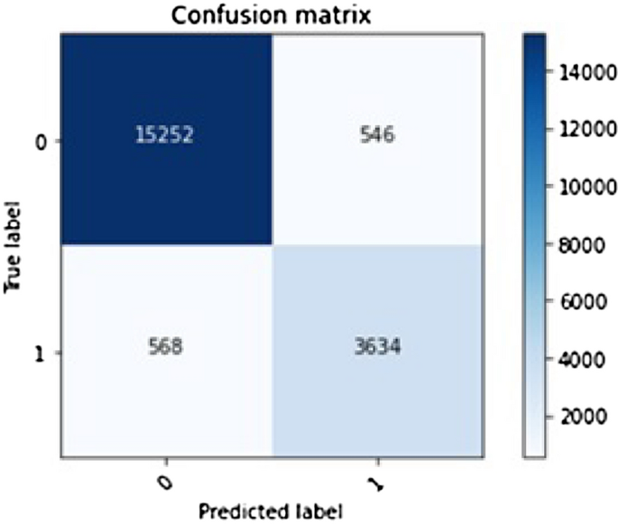

  

  Confusion matrix for ANN

  Table 11 Individual accuracy estimations

  Table 12 Comparative results

From Tables 11 and 12, as one can observe in the aggregated results, it is evident that ANN as one can observe in the aggregated results, it is evident that ANN performs better. Precision represents the avoidance of false positives. It is to be noted that the transformation process introduced in the proposed study plays a significant role in this accuracy analysis concerning both diagnostic and procedural aspects of MIMIC III data. In the model, which we are trying to build, both precision and recall are essential. If the model predicts that the patient is at risk, additional care is required. And in the field of healthcare, more care does not necessarily mean better care. For example, to test tumours, doctors usually employ biopsies. However, this procedure might cause some infection and pain for the patient. To avoid secondary symptoms due to extra procedures performed, the system must be exact. Simultaneously, the system should accurately predict the risk for a patient so that additional procedures must be performed to avoid risk. Hence, the system must have high precision and recall. As we can see in the above graph, ANN has high precession and recall and a high F1 score. And so, we can conclude that ANN is an efficient method to predict risk. In the future, more research must be conducted to predict when a patient can get at risk and predict the patient’s mortality using the same dataset.

6 Conclusion

This research discussed about a novel feature engineering process being carried out over the MIMIC-III dataset. The goal is to extract significant features from the MIMIC III dataset to develop a suitable machine learning system capable of computing anticipated risk. The feature’s correlation is regarded to perform the study associated with different forms of independent predictors. The proposed research uses various independent predictors that are extremely adaptable and can be altered at any time. Scripted in Python, the research outcome shows that ANN offers higher accuracy performance than the other standard machine learning systems.

References

Alshwaheen TI, Hau YW, Ass’ad N, AbuAlSamen MM (2020) A novel and reliable framework of patient deterioration prediction in intensive care unit based on long short-term memory-recurrent neural network. IEEE Access. https://doi.org/10.1109/access.2020.3047186
Bauder RA, Khoshgoftaar TM, Richter A, Herland M (2016) Predicting medical provider specialties to detect anomalous insurance claims. In: 2016 IEEE 28th International Conference on Tools with Artificial Intelligence (ICTAI), pp 784–790. IEEE. https://doi.org/10.1109/ictai.2016.0123
De Georgia MA, Kaffashi F, Jacono FJ, Loparo KA (2015) Information technology in critical care: review of monitoring and data acquisition systems for patient care and research. Sci World J. https://doi.org/10.1155/2015/727694
El-Rashidy N, El-Sappagh S, Abuhmed T, Abdelrazek S, El-Bakry HM (2020) Intensive care unit mortality prediction: An improved patient-specific stacking ensemble model. IEEE Access 8:133541–133564. https://doi.org/10.1109/access.2020.3010556
Ergüzen A, Ünver M (2018) Developing a file system structure to solve healthy big data storage and archiving problems using a distributed file system. Appl Sci 8(6):913. https://doi.org/10.3390/app8060913
Freudenheim M (2002) Some tentative first steps towards universal health care. New York Times 100:1
Gardner RM, Clemmer TP, Evans RS, Mark RG (2014) Patient monitoring systems. Biomedical Informatics. Springer, Berlin, pp 561–591
Ghassemi M, Wu M, Hughes MC, Szolovits P, Doshi-Velez F (2017) Predicting intervention onset in the icu with switching state space models. AMIA Summits on Translational Science Proceedings 2017, 82
Jin Y, Deyu T, Yi Z (2011) A distributed storage model for ehr based on hbase. In: 2011 International Conference on Information Management, Innovation Management and Industrial Engineering, vol. 2, pp. 369–372. IEEE. https://doi.org/10.1109/iciii.2011.234
Johnson AE, Pollard TJ, Mark RG (2017) Reproducibility in critical care: a mortality prediction case study. In: Machine Learning for Healthcare Conference, pp. 361–376. PMLR
Kelly CJ, Karthikesalingam A, Suleyman M, Corrado G, King D (2019) Key challenges for delivering clinical impact with artificial intelligence. BMC Med 17(1):1–9
Krishnan GS (2019) Evaluating the quality of word representation models for unstructured clinical text based icu mortality prediction. In: Proceedings of the 20th International Conference on Distributed Computing and Networking, pp. 480–485. https://doi.org/10.1145/3288599.3297118
Mark R (2016) The story of mimic. Secondary Analysis of Electronic Health Records pp. 43–49. https://doi.org/10.1007/978-3-319-43742-2_5
Moor M, Rieck B, Horn M, Jutzeler C, Borgwardt K (2020) Early prediction of sepsis in the icu using machine learning: A systematic review. medRxiv. https://doi.org/10.1101/2020.08.31.20185207
Nguyen P, Tran T, Wickramasinghe N, Venkatesh S (2016) Deepr: a convolutional net for medical records. IEEE J Biomed Health Inform 21(1):22–30
Physionet: MIMIC-III Website. https://www.physionet.org/ (2008). [Online; accessed 19-July-2020]
Shi Z, Zuo W, Liang S, Zuo X, Yue L, Li X (2020) Iddsam: an integrated disease diagnosis and severity assessment model for intensive care units. IEEE Access 8:15423–15435. https://doi.org/10.1109/access.2020.2967417
Singh A, Guntu M, Bhimireddy AR, Gichoya JW, Purkayastha S (2020) Multi-label natural language processing to identify diagnosis and procedure codes from mimic-iii inpatient notes. arXiv preprint arXiv:2003.07507
Snyderman R, Williams RS (2003) Prospective medicine: the next health care transformation. Acad Med 78(11):1079–1084. https://doi.org/10.1097/00001888-200311000-00002
Sun Y, Guo F, Kaffashi F, Jacono FJ, DeGeorgia M, Loparo KA (2020) Insma: An integrated system for multimodal data acquisition and analysis in the intensive care unit. J Biomed Inform 106:103434. https://doi.org/10.1016/j.jbi.2020.103434
Tran T, Luo W, Phung D, Gupta S, Rana S, Kennedy RL, Larkins A, Venkatesh S (2014) A framework for feature extraction from hospital medical data with applications in risk prediction. BMC Bioinformatics 15(1):1–9. https://doi.org/10.1186/s12859-014-0425-8
Veith N, Steele R (2018) Machine learning-based prediction of icu patient mortality at time of admission. In: Proceedings of the 2nd International Conference on Information System and Data Mining, pp 34–38 . https://doi.org/10.1145/3206098.3206116
Villani C, Rondepierre B (2020) Artificial intelligence and tomorrow’s health. In: Healthcare and Artificial Intelligence, pp. 1–8. Springer. https://doi.org/10.1007/978-3-030-32161-1_1
Walczak S (2018) The role of artificial intelligence in clinical decision support systems and a classification framework. Int J Comput Clin Practice (IJCCP) 3(2):31–47. https://doi.org/10.4018/978-1-7998-1754-3.ch008
Wang S, McDermott MB, Chauhan G, Ghassemi M, Hughes MC, Naumann T (2020) Mimic-extract: A data extraction, preprocessing, and representation pipeline for mimic-iii. In: Proceedings of the ACM Conference on Health, Inference, and Learning, pp 222–235. https://doi.org/10.1145/3368555.3384469
Yamasaki K, Hosoya R (2018) Resolving asymmetry of medical information by using ai: Japanese people’s change behavior by technology-driven innovation for japanese health insurance. In: 2018 Portland International Conference on Management of Engineering and Technology (PICMET), pp 1–5. IEEE. https://doi.org/10.23919/picmet.2018.8481824
Yu K, Zhang M, Cui T, Hauskrecht M (2020) Monitoring icu mortality risk with a long short-term memory recurrent neural network. In: Pacific Symposium on Biocomputing. Pacific Symposium on Biocomputing, vol. 25, pp 103–114. World Scientific
Zeng X, Feng Y, Moosavinasab S, Lin D, Lin S, Liu C (2020) Multilevel self-attention model and its use on medical risk prediction. In: Pac Symp Biocomput. World Scientific
Zikos D, DeLellis N (2018) Cdss-rm: a clinical decision support system reference model. BMC Med Res Methodol 18(1):1–14. https://doi.org/10.1186/s12874-018-0587-6
Acknowledgement
None - No funding to declare.
Funding
Not Applicable (No funding to declare).
Author information
Authors and Affiliations
Corresponding author
Ethics declarations
Conflict of interest
Not applicable.
Ethical Approval and Consent to Participate
Got the access of MIMIC-III data as per the prerequisite from https://physionet.org/. All the data is available to access freely over PhysioNet repository
Consent for Publication
Rights and permissions
Open Access This article is licensed under a Creative Commons Attribution 4.0 International License, which permits use, sharing, adaptation, distribution and reproduction in any medium or format, as long as you give appropriate credit to the original author(s) and the source, provide a link to the Creative Commons licence, and indicate if changes were made. The images or other third party material in this article are included in the article's Creative Commons licence, unless indicated otherwise in a credit line to the material. If material is not included in the article's Creative Commons licence and your intended use is not permitted by statutory regulation or exceeds the permitted use, you will need to obtain permission directly from the copyright holder. To view a copy of this licence, visit http://creativecommons.org/licenses/by/4.0/.
About this article
Cite this article
Khope, S.R., Elias, S. Critical Correlation of Predictors for an Efficient Risk Prediction Framework of ICU Patient Using Correlation and Transformation of MIMIC-III Dataset. Data Sci. Eng. 7, 71–86 (2022). https://doi.org/10.1007/s41019-022-00176-6
Received:
Revised:
Accepted:
Published:
Issue Date:
DOI: https://doi.org/10.1007/s41019-022-00176-6