
Abstract
Recently, metaheuristic approaches are frequently used to the potential data inversion (i.e., magnetic data) as a global optimizing approach. In the present study, we proposed a global optimizing bat algorithm (GOBA) that based on bat echolocation behavior to obtain globally optimal solutions (best parameters) of magnetic anomalies. The best determined source parameters were picked at the suggested minimum objective function. The proposed GOBA approach does not require prior information and represents an effective technique of surveying the entire domain of the raw data to evaluate sources optimal parameters. The GOBA approach is employed to magnetic data profiles to determine the characteristic source attributes (i.e. the vertical depths to the center of the anomalous structures, the magnitude of amplitude coefficients, the sources origin, the approximated geometric form factors, and the effective angles of magnetization). The GOBA approach can be applied to single and multiple anomaly structures in the restricted categories of basic geometric shapes (spheres, cylinders, sheets, and dikes). The stability, constancy, and performance of the given GOBA approach are achieved on different purely and contaminated examples for individual and double sources. Besides, the introduced GOBA approach has been fruitfully utilized to three field datasets from Turkey, Canada, and Senegal for ore deposit and basement rock intrusion investigations. Overall, the recovered inversion results from the GOBA approach are in high correlation with the available drill-holes, geologic data, and scholarly articles outcomes. Finally, the provided metaheuristic GOBA approach is a simple, accurate, and powerful technique for magnetic data interpretation.
Article highlights
-
An automatic approach for magnetic data interpretation to investigate the ore deposits and sustainable resources such as volcanic and basement rock intrusions based on bat echolocation behavior to obtain the global optimal solutions.
-
In this study we built 2D models aims to image of the interior of the subsurface to investigate their natural resources, for example minerals & ore deposits and rock intrusions, helping in understand their concentration and the distribution location, including the depth to their sources.
-
We came to the conclusion that the suggested approach is useful in ore & mineral research, the reconnaissance geological studies and can be extend to the volcanic activity & geothermal exploration studies in the future.
1 Introduction
In the recent years, magnetic techniques have been more important in geothermal research, engineering applications that benefit the environment, archaeology research, unexploded ordnances delineation (UXO), and geotectonic visualization (Hinze 1990; Linford et al. 2019; Elhussein and Shokry 2020; Fkirin et al. 2021; Liu et al. 2021; Nyaban et al. 2021; Hasan et al. 2022). Moreover, a variety of uses for magnetic technology exist for identifying the economic targets including mineral resources and hydrocarbons (Sharma 1987; Gunn and Dentith 1997; Abdelrahman et al. 2007a, b; Mandal et al. 2014; Essa et al. 2018, 2022; Lu et al. 2021).
In the discipline of exploratory geophysics, the investigation and elucidation of magnetic data anomalies appraised along with profiles by some geometrically simple models (spheres, cylinders, sheets, and dikes) continue to be of importance in interpreting the buried magnetized sources (Rao et al. 1981; Abdelrahman and Essa 2015; Biswas 2016; Biswas and Acharya 2016; Essa and Elhussein 2019; Mehanee et al. 2021). Using these simple geometrical models, magnetic data analysis methods have been developed using a variety of graphical and numerical methods. For instance, the approaches using characteristic points, nomograms, and matching curves (Gay 1963; McGrath and Hood 1970; Dondurur and Pamuku 2003; Subrahmanyam and Prakasa Rao 2009), Deconvolution techniques of Euler and Werner (1953; Melo and Barbosa 2020), moved averaging techniques (Abdelrahman et al. 2003), least-squares approaches (Abo-Ezz and Essa 2016), Fourier transforms (Ram Babu and Rao Atchuta 1991; Nuamah and Dobroka 2019), alternative local wave number technique (Ma and Li 2013), numerical gradient-based technique (Essa and Elhussein 2017), tilt-angle methods (Salem et al. 2008; Cooper 2016), correlation techniques (Ma et al. 2017), and spectral analysis techniques (Al-Garni 2011; Kelemework et al. 2021). Though, the majority of these techniques have drawbacks, including the subjectivity involved in data interpretation, the utilization of part of interest data along the deliberate profile, the hyper-sensitiveness to the different noises present in magnetic data, the influence of adjacent effects that may reduce the accuracy of the results, and the reliance on a priori information, that is not constantly available.
In contrast, metaheuristic algorithms, which rely on finding the global optimal solution and are more precise and effective than graphical and numerical approaches, were created to analyze the geomagnetic data. These algorithms including the techniques of simulated annealing algorithm (SA) (Biswas and Rao 2021), genetic algorithm (GA) (Sohouli et al 2022), particle swarm optimization method (PSO) (Essa and Elhussein 2018, 2020; Pace et al. 2021; Heidari et al. 2022), differential evolution algorithm (DE) (Du et al. 2021), ant colony optimization algorithm (ACO) (Yu et al. 2021) and Manta Ray Foraging Optimizing algorithm (Ben et al. 2022). The reason these algorithms are so well-liked by researchers is because, compared to conventional approaches, they are more flexible and capable of handling a variety of issues. The suggested GOBA technique in the current work belongs to the category of metaheuristic algorithms and provides a novel method of analyzing the magnetic data.
In the current work, we implemented the approach of GOBA to interpret the magnetic data measured along 2D profiles using specific elementary geometric forms in the category of spherical shaped models, infinitely long horizontal cylinders, thin sheets, as well as the source of multiple models. The study's objective of the current GOBA approach is represented in inverting the observed data of magnetic anomaly to determine the causal buried body's properties, which are stated in the vertical depth from surface to the center (z), the position of structure origin (xo), the magnitude of amplitude coefficient (K), the effective magnetizing angle (θ), as well as form factors of the structure (q). The recommended interpretative model parameters are attained to match the minimal normal root mean square error (NRMSE) of the given objective function as the software approaches the global best solution. Numerous numerical examples of specific geometric forms are used to test the suggested GOBA technique (spheres, cylinders, and sheets), and multiple-source models as well as is applied to different field cases for ore & mineral deposits as well as the basement rock intrusion.
The accompanying work is coordinated as takes after: Sect. 2 comprises the basics of echolocation as well as the ordinary definition of the bat calculation. The forward modelling and formulation of the suggested GOBA technique are covered in Sect. 3, and the utilizing of GOBA scheme to invert the observed data of magnetic anomaly is covered in Sect. 4. In Sect. 5, it is stated that the recommended GOBA technique has been verified on many numerical instances, both with and without noises, and that the interference multiple model effect has been examined. The applicability of the suggested GOBA technique on numerous real-case examples from diverse fields is demonstrated and discussed in Sect. 6. The conclusion of Sect. 7 concludes by summarizing the goal of the current GOBA technique.
2 The global optimizing bat algorithm
The global optimizing bat algorithm (GOBA), a naturally-inspiration metaheuristic optimizing method, was developed by Yang (2010), and we implemented it to magnetic data interpretation. The GOBA is dependent on the echolocation attribute of bats. In the dark, bats utilised echolocation to find their colony, navigate hazards, and locate prey. The strong sound pulse produced by these bats (8–10 kHz) is used to detect echoes that reflected from adjacent targets. Every pulse scarcely endures a couple of milliseconds (i.e., 8–10 ms). The bats' pulse rates rise as they get closer to prey or an object, but their voice volume decreases (Yang 2010). As a result, it is possible to depict the echolocation behaviour of microbats in a manner which optimizes or maximizes objective functions. The following are the main tenets of the GOBA: (1) Bats utilize sonar to quantify the distance; and (2) Bats fly within a specific frequency band [Qmin, Qmax] to pick up on their surroundings with a primary velocity of (Vi) at location (Xi); and (3) the loudness (Li) & emission rate of pulses, (ri), which differ relied on the gap or separation in the midst of the objective item and the bat.
The movement domain of the bats in the optimization problem may be altered by varying the frequency or wavelength. Therefore, choosing the right frequency is essential. It needs to be selected such that it complements the size of the interest zone before being toned down to lower limits. After utilizing the approach with various settings, the optimal frequency range for the inquiry was found to be in the spectrum of [0, 5 Hz] (Fig. 1). The range of the pulse rate, ri, is [0–1], with 0 meaning no pulses emits and 1 signifying the greatest emission rate of the pulses. Additionally, Li may frequently be in the [1, 2] range for the initial loudness (Yang 2010). The bats' loudness decreases but their rate of pulse emission increases as they draw closer to their target. When a new solution is developed, the algorithm reupdates the emission rate and loudness of the bats, indicating that the bats have found the optimal option (Fister et al. 2013; Essa and Diab 2022).

The effect of different sets of optimization parameters (Qi, Li and ri) on the convergence rate of the GOBA approach technique
The GOBA technique convergence behavior and rate were examined (Fig. 1) utilizing various ranges of the optimum parameters, frequency (Qi), loudness (Li), and rate of pulse emission (ri). According to Fig. 1, the best set is one with (Q1 = [0, 5], L1 = 1, and r1 = 0.9), because it delivers speedy convergence to the optimal solution and has the least NRMSE of the objective function in comparison to other sets. Take note that at the start of the GOBA approach inversion procedure, the starting speed (Vi) at location (Xi) was set to zero.
The following equations demonstrate the relationship between algorithmic parameters (Yang 2010):
where, Qi stands for the ith bat's spectrum frequency, which is updated during each iteration process, \(\beta\) stands for a uniform distributed random arbitrary vector in the domain of [0, 1] and Xbest stands for the actual best global solution obtained from all the bats, \(\alpha\) and \(\gamma\) are constants their values lies between 0 < \(\alpha\) < 1 and \(\gamma\) > 0 and \(\tau\) stand for a scaling factor.
For each best result in the local search, the GOBA method exploits a haphazard track to create new outcomes as shown below:
where Lt stand for the average or main loudness of all bats number at the currently running process, and \(\epsilon\) \(\in\) [-1, 1] stands for a random integer.
3 Forward modeling of magnetic formula
The observed magnetic effect (T) at fixed points (xj) in conjunction with profiles of fundamental geometrically formed entities within the framework of sphere, cylinder, and sheet models (Fig. 2) is provided by (Gay 1963; Rao and Subrahmanyam 1988; Abdelrahman et al. 2012; Mehanee et al. 2021):
where xj stands for the fixed points profile distances (in meters), xo denotes covered source's origin (in meters) (Fig. 2), z stands for the vertical depth to the center of the covered source (in meters) (Fig. 2), θ stands for the effective magnetization angle (in degrees), q denotes the shape factor (unitless), K stands for the amplitude coefficient (nT m2q−2), Table 1 provides a detailed description of the A, B, and C parameters, and n stands for the data point numbers along the profile.

Geometrical shaped model configurations: (a) sphere model, (b) infinite horizontal cylinder model, and (c) thin sheet model
4 Methodology
When interpreting the magnetic data, it is vital to get the truthful parameters for the subsurface model that matching the measured data. In order to produce accurate estimates of the parameters of the underground model, including the depth, location and form of the anomalous body of the buried structure, a large-capacity inversion procedure is necessary. Metaheuristic inversion techniques have shown to be efficient in a number of case studies.
In this study, we have implemented the GOBA to invert magnetic data. The most important parameters that characterize the magnetic data anomaly are depth (z), location (xo), effective magnetization angle (θ), body shape (q), and amplitude coefficient (K). Therefore, in the current GOBA inversion approach, these factors are studied to find an underground model which corresponds to the actual data. The ideal best arrangement solution is found at the place where the objective goal function's NRMSE has the lowest misfit error (Xbest). Following that, the GOBA inversion program was tested on a range of synthetic numerical examples in this research. Following that, it was put to the test on different actual-field examples.
The suggested GOBA method is composed of the following phases are utilized to invert the magnetic data:
-
(1)
Initial location Xi (i = 1, 2, 3,…, N), frequencies Qi, speed or velocities Vi, loudness Li, as well as emission rate of pulses ri of the virtual bats are takes after: Each bat signifies a possible solution in the pursuit space. The variable Xi is depicted by the characteristic model attributes (i.e., z, xo, K, θ, and q) are picked at random from the searching space, and Vi denotes the speed of each virtual bat,
-
(2)
Discover the Xbest,
The objective function is the NRMSE between calculated and observed magnetic anomalies (\(\psi\)) or the misfit and is expressed as:
$$\psi =100\sqrt{\frac{1}{N}\sum_{j=1}^{N}{\left[\frac{{T}_{Obs}-{T}_{Cal}}{{T}_{Obs}}\right]}^{2}}$$(8)where, N characterizes the data point numbers, TObs stands for the observed magnetic data and TCal stands for the calculated magnetic model response. Equation 8 is used to assess the misfits first, and The Xbest bat is determined to be the one with the least misfit or mismatch.
-
(3)
while the programme has not yet gone through the maximum number of iterations, execute the next set of instructions:
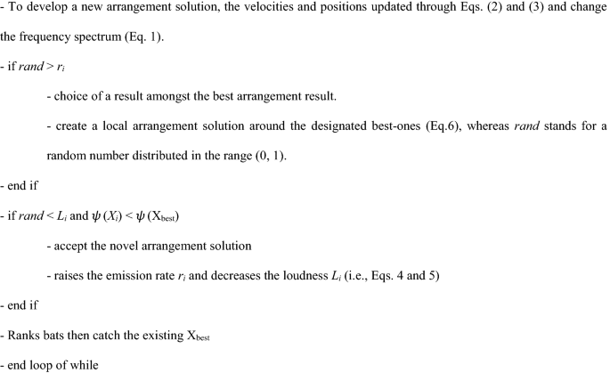

The fundamental components of the GOBA approach can be framed in the flow diagram delineated in Fig. 3.

Flowchart shows the essential elements of the GOBA approach
5 Numerical dataset examples
The suggested GOBA approach was examined on various numerical dataset examples to determine its efficiency and validity in understanding and inverting the magnetic data. These numerical examples depend on using simple geometrical shapes models (spheres, cylinders, and sheets). The suggested approach is tested to noise-free example first and contaminated with noise to show the effectiveness and durability of the proposed approach. Moreover, it investigated the interference impact of multi-neighboring structures.
5.1 Case model 1
Initially, free of noise numerical case of an infinite horizontally cylinder source model with the taking after specifications K = 3000 nT m2, z = 15 m, xo = 0 m, θ = -55 ̊ and q = 2.0 has been investigated (Fig. 4a) using the procedures of the GOBA approach introduced in Sect. 2. Figure 4b plots the average loudness of the bats vs iteration counts. Figure 4c displays the bats’ emission rate generated at every iteration operation, where the pulse emission rate rises, and the bats' loudness increases as they draw closer to their prey. Figure 4d plots the NRMSE of the lowest objective function, of the global best solution, against the number of iterations. It can be seen from the figure that all bat numbers reach the min after 300 iterations. The average value of NRMSE of all numbers of the bats acquired during each iterative process is shown in Fig. 4e.

Noise-free numerical example of the infinite horizontal cylinder model (case Model-1); (a) The measured magnetic anomaly generated by horizontal cylinder model (True model parameters), as well as the calculated magnetic anomaly (Recovered model parameters) using the GOBA approach, (b) loudness of the bats, (c) emission rate of the bats, (d) NRMSE of the global best solution (\(\psi\)) of the bats versus the iteration numbers, and (e) the average NRMSE of all the bats
When the objective function (\(\psi\)) during the iteration process achieves the lowest value of the NRMSE, the magnetic anomaly's global best solution (i.e., the source model attributes) are obtained. Table 2 shows that the provided noise-free example's evaluated model attributes match those of the actual model attributes exactly. This implies that the conducted GOBA approach is accurate, firm, and capable of retrieving acceptable outcomes of the attributes of the given model. Additionally, Table 2 displays the search rang or space and relative errors (RE) for every model parameter.
With varying levels of noise (10 and 15%), we added two distinct types of noise, first the additive white Gaussian noise (AWGN) and second the Gaussian random noise (GRN) to the data free of noise shown in Fig. 4a to assess the robustness of the current GOBA technique. The optimum model parameters were discovered at the lowest NRMSE of the objective goal function (\(\psi\)) by using the GOBA scheme's aforementioned procedures to the erratic data anomaly patterns. Figure 5 displays the noisy polluted magnetic anomaly that resulted from the 10% and 15% GRN being added to the data (Fig. 4a), together with the computed magnetic response (frame a). Frames (b), (c), (d), and (e) of Fig. 5 show, in turn, the curve of loudness, the curve of pulse rate of emission, NRMSE of the best global arrangement solution (\(\psi\)), and the average values of NRMSE of all number of the bats.

Noisy numerical example of the infinite horizontal cylinder model (case Model-1: Fig. 4a) after contaminated with 10% GRN (I) and 15% GRN (II); (a) Noisy magnetic anomaly generated by horizontal cylinder model (True model parameters) and the calculated magnetic anomaly (Recovered model parameters) using the GOBA approach, (b) loudness of the bats, (c) emission rate of the bats, (d) NRMSE of the global best solution (\(\psi\)) of the bats versus the iteration numbers, and (e) the average NRMSE of all the bats
After including the 10% & 15% of the AWGN noise type into the generated data (Fig. 4a), Fig. 6 displays the polluted magnetic data as well as the predicted magnetic response (frame (a)). Frames (b), (c), (d), and (e) of Fig. 6 show the loudness curve, the pulse rate emission curve, the NRMSE of the best global arrangement solution (\(\psi\)), respectively, and the average values of the NRMSE of all numbers of the bats. The associated retrieved attributes or parameters for the noisy cases for both forms of injected noises (GRN & AWGN) and their percentages are displayed in Tables 3 and 4. The derived parameters are so near to the real ones that they are not considerably impacted by the forms of intruded noise. Additionally, Tables 3 and 4 show the RE related to every model attribute that was derived for each type of given noise. Finally, it may be inferred that the GOBA technique recommended here is steady in regard to the different kind of noise.

Noisy numerical example of the infinite horizontal cylinder model (case Model-1: Fig. 4a) after contaminated with 10% AWGN (I) and 15% AWGN (II); (a) Noisy magnetic anomaly generated by horizontal cylinder model (True model parameters) and the calculated magnetic anomaly (Recovered model parameters) using the GOBA approach, (b) loudness of the bats, (c) emission rate of the bats, (d) NRMSE of the global best solution (\(\psi\)) of the bats versus the iteration numbers, and (e) the average NRMSE of all the bats
5.2 Case model 2
In some geologic environments, the interference effects (i.e. the activity of surrounded numerous source structure) might affect the collected magnetic data of an anomalous confined hidden source structures. As a result, we used Eq. 7 to compute the composite magnetic effect for two nearby sources, also known as the infinite horizontal cylinder model with true parameters [K1 = 1500 nT m2, z1 = 12 m, xo1 = −50 m, θ = -35° and q1 = 2] as well as a spherical source model has the taking after actual attributes [K2 = 10,000 nT m3, z2 = 10 m, xo2 = 50 m, θ = −35° and q2 = 2.5], along a profile with 201 m length (Fig. 7a) to test the influence of these double interference sources on the precision of the inverted model attributes elucidated utilizing the current GOBA technique. The observed magnetic anomaly of the two models is shown in Fig. 7a using the aforementioned GOBA approach processes. Figure 7b displays the composite anomaly's calculated average loudness curve, and Fig. 7c displays the bat emission rate. Additionally, Fig. 7d displays the NRMSE of the overall best arrangement solution (\(\psi\)), and Fig. 7e displays the average values of the NRMSE of all numbers of the bats. The obtained model attributes of these two neighboring source bodies or structures, which are quite similar to the genuine input ones, are displayed in Table 5. Additionally, Table 5 displays the RE of the retrieved model attributes in relation to every source bodies. The outcomes demonstrate that the GOBA technique is firm and accurate even in the case of multi-sources.

Interference and multiple structure effect (case Model-2); (a) The composite magnetic anomaly generated by infinite horizontal cylinder and sphere model (True model parameters), as well as the calculated magnetic response of them (Recovered model parameters) using the GOBA approach, (b) loudness of the bats, (c) emission rate of the bats, (d) NRMSE of the global best solution (\(\psi\)) of the bats versus the iteration numbers, and (e) the average NRMSE of all the bats
In addition, the stability and exactness of the recommended GOBA scheme on multiple source structures and neighbouring influences was checked in case of the field contaminated with various kind of noises (GRN and AWGN) (Fig. 7a). The optimal model parameters were derived using the GOBA approach scheme when the objective goal function's NRMSE (\(\psi\)) was the lowest for the noisy composite anomaly. After including the 10% GRN (Fig. 8I) & 10% of the other noise type of AWGN (Fig. 8II) to the composite magnetic curve displayed in Figs. 7a, 8 displays the polluted composite anomaly curve of the two surrounding source bodies, and their calculated responses after getting the best model attributes (window a). Window (b), (c), (d), and (e) of Fig. 8 show, correspondingly, the loudness, emission rate, global best solution's NRMSE (\(\psi\)), and the average values of the NRMSE of all number of bats.

Noisy interference and multiple structure effect (Case Model-2: Fig. 7a) after contaminated with 10% GRN (I) and 10% AWGN (II); (a) The noisy composite magnetic anomaly generated by infinite horizontal cylinder and sphere model (True model parameters) and the calculated magnetic response of them (Recovered model parameters) using the GOBA approach, (b) loudness of the bats, (c) emission rate of the bats, (d) NRMSE of the global best solution (\(\psi\)) of the bats versus the iteration numbers, and (e) the average NRMSE of all the bats
The inverted attributes of the polluted composite magnetic anomaly are displayed in Tables 6 and 7 for the respective noise types (GRN and AWGN). The estimated characteristics properties of the two contaminated source structures, including both two different kinds of are still very good corresponding to the real ones. The RE related to every computed model attribute for noise of all kinds are also shown in Tables 6 and 7.
It can be concluded from the synthetic data cases displayed over that the GOBA method utilized here is steady and proper for the analysis and clarification of actual magnetic field data, as described in the subsequent section.
6 Real dataset examples
In the following sections, we have studied the applicability of the GOBA approach on three published magnetic data field examples as follows; the first case is the Cataldere magnetic effect from Turkey on magnetite ore & mineral resources in the Bala district. The Faro magnetic anomaly from Canada for the lead–zinc deposit in the Yukon territory is the second case. The third case is the West Coast magnetic anomaly from Senegal for the basement rock intrusion.
6.1 Case example 1: The Cataldere magnetic anomaly, Bala district, Turkey
The Bala district includes five iron ore deposits with 400–2000 thousand tone reserve. These deposits are located within a magnetite-mineralization zone that covers a total area of 25 km2 and has similar mineralogical and geological properties. Ozturk et al. (1983) proposed that “the magnetite ore in this district skarn regions resulted from a meta-somatic hydrothermal interaction between marble layers and acidic materials”. The orebodies are made up of 90% magnetite and 10% specularite, limonite, and hematite. In the district, there are hematite rich regions. Magnetite cores samples came from drillings in this area had susceptibilities ranging from 400 × 10−3 to 1200 × 10−3 SI. The Cataldere anomaly is located on the easternmost side of the Bala district. An alluvial layer of thickness rang 2–3 m covers the whole surface of the land. The province's geography is slightly planed, with elevation less than 7 m.
The skarn zone shows small outcropping magnetite blocks found in limited region east of the drilled-hole C1 (Fig. 11). These magnetite boulders composed the main anomaly’s figure. Furthermore, these blocks have obscured the primary anomaly's pinnacle location as well as the true strength of the positive and negative components (Fig. 9). In the 1970s, old geophysical surveys in the Bala district measured the magnetic field's vertical component strength using a 40 m separation between station and a 200 m of profile length (Kayaoglu and Ozertan 1979). According on this ancient magnetic data, the drilled-holes CD1 and CD7 had recommended and accomplished. The most recent total magnetic field estimations were collected by a proton-type magnetometer with a 1 nT precision between stationary points with varied spacing range from 2 to 10 m across the profiles, which separated by 20 m. Figure 9 depicts the final magnetic anomaly contouring map of the Cataldere area as well as the sites of the most recent drilling.

The Cataldere magnetic anomaly map shown the position of the A–A' profile and the drilling holes location. The drillings cut the iron orebody are shown by solid circles

The Cataldere magnetic anomaly, Bala district, Turkey; (a) The measured magnetic anomaly profile (blue squares) and the calculated best-fitting magnetic response (red circles) using the GOBA approach and the calculated curve by Aydin (2008) method, (b) loudness of the bats, (c) emission rate of the bats, (d) NRMSE of the global best solution (\(\psi\)) of the bats versus the iteration numbers, and (e) the average NRMSE of all the bats
A magnetic profile A–A’ is taken across the Cataldere anomaly in NE-SW direction over the magnetic map (Fig. 9). The Cataldere anomaly profile A–A’ of length 256 m was sampled at 4 m digitizing interval (Fig. 10a). By employing the GOBA processes on the Cataldere magnetic anomaly profile A–A’, the distinctive source attributes of the anomaly were estimated. The average values of the bat loudness plot and the emission rate curve across the magnetic data are depicted in Fig. 10b and c, respectively. Figure 10d and e, respectively, display the NRMSE of the best global arrangement result (\(\psi\)) and the average values NRMSE of all number of bats. The model attributes that can be best comprehended are those that match the minimum (\(\psi\)). The min (\(\psi\)) is 11.8 and the corresponding optimal parameters of the response model are [K = 7,600,000 ± 726.27 nT m2, z = 62 ± 4.00 m, xo = 20 ± 1.87 m, θ = −70° ± 4.08 and q = 2 ± 0.01], which proposes that the effect of the Cataldere anomaly be similar to a horizontal cylinder-like model. Figure 10a shows that the estimated and measured magnetic anomalies agree well.
The Cataldere magnetic anomaly profile A–A' was interpreted by Aydin (2008) using analytic signals method as a triangle model with three depths 90, 30, and 20 m represent the triangle corners. The current work of GOBA scheme interpreted the Cataldere magnetic anomaly approximated by horizontal cylinder body at depth to the center to the subsurface ore body deposit about 62 m, which agrees very well with the drilling information (C1, CD1, and C3 of Fig. 11). Additionally, the present GOBA scheme has RMS error (217 nT) amongst the observed and calculated anomaly, which is less than the RMS error (259 nT) achieved by Aydin (2008) method (Fig. 10a). The slightly large values in the RMS error (i.e., the mismatch) between the measured and calculated anomalies are due to the interpretation was done directly on the observed anomaly not on the residual one.

(a) Cataldere magnetic profile A–A' (from SW to NE) and the interpreted calculated response using the present study and other published technique (Aydin 2008). (b) Drilling cross-section showing iron ore deposits and the computed models using the present approach and Aydin (2008) technique. The plus sign indicates the source position
6.2 Case example 2: The Faro magnetic anomaly, Yukon, Canada
The Faro Mine lies 15 km north of Faro, in the south-central Yukon Region in northern Canada (Tang 2011). The geography of this region is dictated by the Yukon Plateau and the adjacent Anvil Range Mountains, which have altitudes exceeding 1800 m. The Faro Mine lies in the northern west area of the Faro Complex zone (Fig. 12) and its regional geology described by the geologic information of the Anvil territory (Fig. 13). A geophysical survey was conducted over the Faro district area including both magnetic as well as gravity measurements to discover the ore deposits in the area. The magnetic effect over the Faro deposit (Fig. 14a) provided shallow gradient anomaly (Reynolds 1997). The ore deposit of Faro (i.e. lead–zinc sulphide ore resource) locates nearby 100 m beneath the Mount Mye Vangorda boundary (Fig. 14b).

The location map of the Faro Mine Complex, Canada with site layout (sourced from, Tang 2011)

The Geology of Canada's Anvil District (Tang 2011). The Faro sulphide deposit is depicted in this diagram

The hosted rocks, so called the Mount Mye rock Formation, has been transformed to biotite muscovite schist, while the Vangorda rock Formation has been altered to thick, banded calcsilicate (Brock 1973). According to Brock (1971), the initial estimates during the exploratory step (with the ore density equals 3.65 g/cc and the host rocks is 2.75 g/cc) yielded a 44 M tons-mass, which was later compared to a proved drilling recovery of roughly 46 M tons (Brock 1971, 1973; Tanner and Gibb 1979).
A 12-m sampling interval was used to digitize an 805-m magnetic profile collected over the "Faro No. 1 Deposit" (Fig. 15a). The Faro magnetic anomaly profile is interpreted using the present GOBA approach by applying the previously mentioned procedures and hence the source attribute parameters of the anomaly can be determined. Figure 15b and c, respectively, display the bat's average values loudness curve and the emission rate curve across the magnetic effect. In Fig. 15d and e, the NRMSE of the best global arrangement solution (\(\psi\)) and the average values of the NRMSE of all number of the bats, sequentially, are displayed. The best determined model attributes that can be retrieved are found to match the minimum (\(\psi\)). The min (\(\psi\)) = 10.49 and the best interpreted model attributes for the matching data are [K = 7,200,000 ± 599.30 nT.m2, z = 173 ± 2.44 m, xo = −70 ± 23.11 m, θ = −20° ± 3.35 and q = 2 ± 0.40], which recommended that the Faro anomaly source is roughly represented by cylinder-shaped horizontal model. Figure 15a illustrates how well the estimated and measured magnetic anomalies of the Faro correspond.

The Faro magnetic anomaly, Yukon, Canada; (a) The measured magnetic anomaly profile (blue squares) and the calculated best-fitting magnetic response (red circles) using the GOBA approach, (b) loudness of the bats, (c) emission rate of the bats, (d) NRMSE of the global best solution (\(\psi\)) of the bats versus the iteration numbers, and (e) the average NRMSE of all the bats
The gravity anomaly that collected by the geophysical survey over the Faro district area have been interpreted using the R-parameter imaging technique (Essa et al. 2020) mentioned that the Faro anomaly has a depth to the center equals 195 m and the form of the anomaly is approximated as cylinder-shaped horizontal model. The present GOBA approach interpreted the Faro anomaly at depth extended from the surface to the center of the uncovered ore source about 173 m, which in turn matched greatly with the geologic and drill-holes data (Fig. 14b), as well as gives good integration with the published results of the gravity field of the Faro anomaly (Essa et al. 2020).
6.3 Case example 3: The West Coast magnetic anomaly, Senegal, West Africa
Figure 16a depicts a large magnetic anomaly (total field) detected along Senegal's western coast in West Africa (Nettleton 1976). The magnetic profile's reference line and zero intersection were supplied by Nettleton (1976) as well as Rao and Subrahmanyam (1988). The causal body, according to Nettleton (1976), is a basic basement rock intrusion. The magnetic profile of the length of 40 km was sampled at 0.5 km intervals (Fig. 16a).

The West Coast magnetic anomaly, Senegal, West Africa; (a) The measured magnetic anomaly profile (blue squares), and the calculated best-fitting magnetic response (red circles) using the GOBA approach and the calculated curve by Mehanee et al. (2021) method, (b) loudness of the bats, (c) emission rate of the bats, (d) NRMSE of the global best solution (\(\psi\)) of the bats versus the iteration numbers, and (e) the average NRMSE of all the bats
Figure 16b–e illustrates, in accordance with the GOBA approach's processes, the loudness, emission rate, global best solution's NRMSE (\(\psi\)), and the average values of the NRMSE of all numbers of the bats. The min (\(\psi\)) values correspond to the best interpretative model parameters (\(\psi\) = 9.2) are K = 463,000 ± 16.09 nT.km3, z = 10 ± 0.17 km, xo = 9 ± 0.48 km, θ = 19.3° ± 0.34 and q = 2.5 ± 0.00, which recommended that the west coast Senegal anomaly is approximated by a sphere-like model. The estimated and measured magnetic anomaly curves of the West Coast of Senegal have outstanding matching as illustrated in Fig. 16a.
The anomaly of West Coast of Senegal has been elucidated by several authors (Table 8). Table 8 compares the results attained by the current GOBA technique to those indicated in the scholarly studies (Nettleton 1976; Rao and Subrahmanyam 1988; Abdelrahman et al. 2007b; Mehanee et al. 2021). The comparison of the attained results shows that the depth and the effective magnetizing angle obtained by the technique described in our research are consistent with those reported in the literature.
7 Conclusions
Calculation of the suitable buried model responses for simulating the subsurface source structures is important in interpretation of magnetic data. To attain the appropriate model parameters (best model), a Global Optimizing Bat algorithm (GOBA) was employed to the magnetic data. After determining the global best arrangement that minimizes the NRMSE misfit of the objective goal function, the best optimized model attributes are derived (i.e. amplitude coefficient, center depth, the place of origin, and model form factors), correlating to the recommended minimal objective function. No prior knowledge is necessary for the GOBA method; the recovered solution is depending on using a search space to search for the model parameters. The GOBA's designed inversion method is straightforward, quick, precise, and easy to use with a variety of magnetic datasets. Moreover, it can handle multi-model problems efficiently. Furthermore, the effectivity and precision of the recommended approach have been verified on synthetic data examples with various noise kinds (GRN & AWGN) and levels (10 & 15%). The GOBA method is then successfully applied to three distinct actual datasets from Turkey, Canada, and Senegal for ore deposit and basement rock intrusion investigations. From the investigations indicated above, we deduced that the suggested method is advantageous for ore and mineral explorations and may be expanded in the future to include geothermal exploration and studies of volcanic activity.
Data availability
The data used are offered upon request from the corresponding author.
References
Abdelrahman EM, Essa KS (2015) A new method for depth and shape determinations from magnetic data. Pure Appl Geophys 172:439–460
Abdelrahman EM, Abo-Ezz ER, Essa KS (2012) Parametric inversion of residual magnetic anomalies due to simple geometric bodies. Explor Geophys 43:178–189
Abdelrahman EM, Abo-Ezz ER, Soliman KS, El-Araby TM, Essa KS (2007a) A least-squares window curves method for interpretation of magnetic anomalies caused by dipping dikes. Pure Appl Geophys 164:1027–1044
Abdelrahman EM, El-Araby TM, Soliman KS, Essa KS, Abo-Ezz ER (2007b) Least-squares minimization approaches to interpret total magnetic anomalies due to spheres. Pure Appl Geophys 164:1045–1056
Abdelrahman EM, El-Arby HM, El-Arby TM, Essa KS (2003) A least-squares minimization approach to depth determination from magnetic data. Pure Appl Geophys 160:1259–1271
Abo-Ezz ER, Essa KS (2016) A least-squares minimization approach for model parameters estimate by using a new magnetic anomaly formula. Pure Appl Geophys 173:1265–1278
Al-Garni MA (2011) Spectral analysis of magnetic anomalies due to a 2-D horizontal circular cylinder: a Hartley transforms technique. SQU J Sci 16:45–56
Aydin I (2008) Estimation of the location and depth parameters of 2D magnetic sources using analytical signals. J Geophys Eng 5:281–289
Ben UC, Ekwok SE, Akpan AE, Mbonu CC, Eldosouky AM, Abdelrahman K, Gómez-Ortiz D (2022) Interpretation of magnetic anomalies by simple geometrical structures using the manta-ray foraging optimization. Front Earth Sci 10:849079. https://doi.org/10.3389/feart.2022.849079
Biswas A (2016) Interpretation of gravity and magnetic anomaly over thin sheet-type structure using very fast simulated annealing global optimization technique. Model Earth Syst Environ 2:30
Biswas A, Rao K (2021) Interpretation of magnetic anomalies over 2D fault and sheet-type mineralized structures using very fast simulated annealing global optimization: an Understanding of uncertainty and geological implications. Lithosphere 2021:2964057. https://doi.org/10.2113/2021/2964057
Biswas A, Acharya T (2016) A very fast simulated annealing (VFSA) method for inversion of magnetic anomaly over semi-infinite vertical rod-type structure. Model Earth Syst Environ 2:198
Brock JS (1971) Geophysical exploration leading to discovery of the Faro deposit, Yukon territory. Presented at the AIME centennial annual meeting, New York, New York, Feb 26–March 4
Brock JS (1973) Geophysical exploration leading to the discovery of the Faro deposit. Can Min Metall Bull 66:97–116
Cooper GRJ (2016) Applying the tilt depth and contact depth methods to the magnetic anomalies of thin dykes. Geophys Prospect 65:316–323
Dondurur D, Pamuku OA (2003) Interpretation of magnetic anomalies from dipping dike model using inverse solution, power spectrum and Hilbert transform methods. J Balk Geophys Soci 6:127–139
Elhussein M, Shokry M (2020) Use of the airborne magnetic data for edge basalt detection in Qaret Had El Bahr area, Northeastern Bahariya Oasis. Egypt Bull Eng Geol Environ 79:4483–4499
Essa KS, Diab ZE (2022) Magnetic data interpretation for 2D dikes by the metaheuristic bat algorithm: sustainable development cases. Sci Rep 12:14206
Essa KS, Elhussein M (2017) A new approach for the interpretation of magnetic data by a 2-D dipping dike. J Appl Geophy 136:431–443
Essa KS, Elhussein M (2018) PSO (particle swarm optimization) for interpretation of magnetic anomalies caused by simple geometrical structures. Pure Appl Geophys 175:3539–3553
Essa KS, Elhussein M (2019) Magnetic interpretation utilizing a new inverse algorithm for assessing the parameters of buried inclined dike-like geologic structure. Acta Geophys 67:533–544
Essa KS, Elhussein M (2020) Interpretation of magnetic data through particle swarm optimization. Mineral exploration cases studies. Nat Resour Res 29:521–537
Essa KS, Munschy M, Youssef MAS, Khalaf EA (2022) Aeromagnetic and radiometric data interpretation to delineate the structural elements and probable precambrian mineralization zones: a case study, Egypt. Min Metall Explor. https://doi.org/10.1007/s42461-022-00675-0
Essa KS, Mehanee SA, Soliman KS, Diab ZE (2020) Gravity profile interpretation using the R-parameter imaging technique with application to ore exploration. Ore Geol Rev 126:103695
Essa KS, Nady AG, Mostafa MS, Elhussein M (2018) Implementation of potential field data to depict the structural lineaments of the Sinai Peninsula, Egypt. J Afr Earth Sci 147:43–53
Fkirin MA, Youssef MAS, El-Deery MF (2021) Digital filters applications on aeromagnetic data for identification of hidden objects. Bull Eng Geol Environ 80:2845–2858
Fister IJ, Fister I, Yang XS (2013) A hybrid bat algorithm. Electrotech Rev 80:1–7
Gay P (1963) Standard curves for interpretation of magnetic anomalies over long tabular bodies. Geophysics 28:161–200
Gunn PJ, Dentith M (1997) Magnetic responses associated with mineral deposits. AGSO J Aust Geol Geophys 17:145–158
Hasan M, Shang Y, Jin W et al (2022) Site suitability for engineering-infrastructure (EI) development and groundwater exploitation using integrated geophysical approach in Guangdong, China. Bull Eng Geol Environ 81:7
Heidari M, Meshinchi Asl M, Mehramuz M, Heidari R (2022) Magnetic field analysis using the improved global particle swarm optimization algorithm to estimate the depth and approximate shape of the buried mass. Contrib Geophys Geod 52(2):281–305. https://doi.org/10.31577/congeo.2022.52.2.6
Hinze WJ (1990) The role of gravity and magnetic methods in engineering and environmental studies. Geotech Environ Geophys 1:75–126
Kayaoglu A, Ozertan M (1979) Magnetometric survey report of the Kırsehir-Kaman district (Kesikkopru). Report no 6739 (Ankara: Mineral Research and Exploration (MTA)) (unpublished, in Turkish)
Kelemework Y, Fedi M, Milano M (2021) A review of spectral analysis of magnetic data for depth estimation. Geophysics 86:J33–J58
Linford N, Linford P, Payne A (2019) Advanced magnetic prospecting for archaeology with a vehicle-towed array of cesium magnetometers. Innov near-Surf Geophys 5:121–149
Liu Y, Xia Q, Cheng Q (2021) Aeromagnetic and geochemical signatures in the Chinese Western Tianshan: implications for tectonic setting and mineral exploration. Nat Resour Res 30:3165–3195
Lu N, Liao G, Xi Y, Zheng H, Ben F, Ding Z, Du L (2021) Application of airborne magnetic survey in deep iron ore prospecting—a case study of Jinling Area in Shandong Province, China. Minerals 11:1041
Ma G, Li L (2013) Alternative local wavenumber methods to estimate magnetic source parameters. Explor Geophys 44:264–271
Ma G, Liu C, Xu J, Meng Q (2017) Correlation imaging method based on local wavenumber for interpreting magnetic data. J Appl Geophy 138:17–22
Mandal A, Mohanty WK, Sharma SP, Biswas A, Sen J, Bhatt AK (2014) Geophysical signatures of uranium mineralization and its subsurface validation at Beldih, Purulia District, West Bengal, India: a case study. Geophys Prospect 63:713–726
McGrath PH, Hood PJ (1970) The dipping dike case: a computer curve matching method of magnetic interpretation. Geophysics 35:831–848
Mehanee S, Essa KS, Diab ZE (2021) Magnetic data interpretation using a new R-parameter imaging method with application to mineral exploration. Nat Resour Res 30:77–95
Melo FF, Barbosa VCF (2020) Reliable Euler deconvolution estimates throughout the vertical derivatives of the total-field anomaly. Comput Geosci 138:104436
Nettleton LL (1976) Gravity and magnetics in oil prospecting. McGraw Hill Book Co, New York
Nuamah DOB, Dobroka M (2019) Inversion-based fourier transformation used in processing non-equidistantly measured magnetic data. Acta Geod Geophys 54:411–424
Nyaban CE, Ndougsa-Mbarga T, Bikoro-Bi-Alou M, Tadjouteu SAM, Assembe SP (2021) Multi-scale analysis and modelling of aeromagnetic data over the Bétaré-Oya area in eastern Cameroon, for structural evidence investigations. Solid Earth 12:785–800
Ozturk K, Kurt M, Ozturk M, Sari I (1983) Report on geological and reserve studies of Ankara-Bala-Kesikkopru, Madentepe, B.Ocak, Cataldere and Camisagir iron ore deposits Report no 7355 (Ankara: General Directorate of Mineral Research and Exploration (MTA)) (Unpublished, in Turkish)
Pace F, Santilano A, Godio A (2021) A review of geophysical modeling based on particle swarm optimization. Surv Geophys 42:505–549
Ram Babu HV, Rao Atchuta D (1991) Application of the Hilbert transform for gravity and magnetic interpretation. Pure Appl Geophys 135:589–599
Rao DA, Babu HVR, Narayan PVS (1981) Interpretation of magnetic anomalies due to dikes: the complex gradient method. Geophysics 46:1572–1578
Rao PTKS, Subrahmanyam M (1988) Characteristic curves for inversion of magnetic anomalies of spherical ore bodies. Pure Appl Geophys 126:69–83
Reynolds JM (1997) An introduction to applied and environmental geophysics. John Wiley and Sons, New York, p 796
Salem A, Williams S, Fairhead D, Smith R, Ravat D (2008) Interpretation of magnetic data using tilt-angle derivatives. Geophysics 73:L1–L10
Sharma PV (1987) Magnetic method applied to mineral exploration. Ore Geol Rev 2:323–357
Sohouli AN, Molhem H, Zare-Dehnavi N (2022) Hybrid PSO-GA algorithm for estimation of magnetic anomaly parameters due to simple geometric structures. Pure Appl Geophys 179:2231–2254. https://doi.org/10.1007/s00024-022-03048-2
Subrahmanyam M, Prakasa Rao TKS (2009) Interpretation of magnetic anomalies using simple characteristics positions over tabular bodies. Explor Geophys 40:265–276
Tang MSM (2011) Delineation of groundwater capture zone for the Faro mine, Faro mine complex, Yukon territory. BSc thesis. The University of British Columbia, Vancouver, Canada
Tanner JG, Gibb RA (1979) Gravity method applied to base metal exploration, in Geophysics and Geochemistry in the Search for Metallic Ores (ed, Hood PJ), Geological Survey of Canada. Econ Geol Report 31:105–122
Werner S (1953) Interpretation of magnetic anomalies of sheetlike bodies. Norstedt, Sveriges Geolologiska Undersok, Series C, Arsbok, 43, no. 6
Du W, Cheng L, Li Y (2021) lp norm smooth inversion of magnetic anomaly based on improved adaptive differential evolution. Appl Sci 11:1072. https://doi.org/10.3390/app11031072
Yang XS (2010) A new metaheuristic bat-inspired algorithm: in Nature Inspired Cooperative Strategies, Gonza´lez J, Pelta D, Cruz C, Terrazas G and Krasnogor N (eds), vol. 284, pp 65–74
Yu J, You X, Liu S (2021) Ant colony algorithm based on magnetic neighborhood and filtering recommendation. Soft Comput 25:8035–8050. https://doi.org/10.1007/s00500-021-05851-w
Acknowledgements
The authors express their gratitude to Prof. P.G. Ranjith, Editor-in-Chief, and the expert reviewer for his/her strong attention, insightful criticism, and changes to this paper to be published in Geomechanics and Geophysics for Geo-Energy and Geo-Resources.
Funding
Open access funding provided by The Science, Technology & Innovation Funding Authority (STDF) in cooperation with The Egyptian Knowledge Bank (EKB). Not applicable for that section.
Author information
Authors and Affiliations
Contributions
EKS: Original Draft Writing, Conceptualization, and Methodology. DZE: creation of the first draught of the paper, testing of the program code, conceptualization, methodology, validation, and creation of the figures and tables.
Corresponding author
Ethics declarations
Conflict of interest
The authors declare there is no conflict of interests.
Additional information
Publisher's Note
Springer Nature remains neutral with regard to jurisdictional claims in published maps and institutional affiliations.
Rights and permissions
Open Access This article is licensed under a Creative Commons Attribution 4.0 International License, which permits use, sharing, adaptation, distribution and reproduction in any medium or format, as long as you give appropriate credit to the original author(s) and the source, provide a link to the Creative Commons licence, and indicate if changes were made. The images or other third party material in this article are included in the article's Creative Commons licence, unless indicated otherwise in a credit line to the material. If material is not included in the article's Creative Commons licence and your intended use is not permitted by statutory regulation or exceeds the permitted use, you will need to obtain permission directly from the copyright holder. To view a copy of this licence, visit http://creativecommons.org/licenses/by/4.0/.
About this article

Cite this article
Essa, K.S., Diab, Z.E. An automatic inversion approach for magnetic data applying the global bat optimization algorithm (GBOA): application to ore deposits and basement rock intrusion. Geomech. Geophys. Geo-energ. Geo-resour. 8, 185 (2022). https://doi.org/10.1007/s40948-022-00492-1
Received:
Accepted:
Published:
DOI: https://doi.org/10.1007/s40948-022-00492-1