Canonical and log canonical thresholds of Fano complete intersections

Abstract

It is proved that the global log canonical threshold of a Zariski general Fano complete intersection of index 1 and codimension k in ${\mathbb P}^{M+k}$ is equal to one, if $M\geqslant 2k+3$ and the maximum of the degrees of defining equations is at least 8. This is an essential improvement of the previous results about log canonical thresholds of Fano complete intersections. As a corollary we obtain the existence of Kähler–Einstein metrics on generic Fano complete intersections described above.

1 Introduction

1.1 Statement of the main result

The aim of the present paper is to show that the global (log) canonical threshold of a general Fano complete intersection of index 1 is at least (respectively, equal to) one, except for a sufficiently narrow class of Fano complete intersections, defined by equations of low degree. More precisely, let $\underline{d}=(d_1,\dots ,d_k)$ be an ordered integral vector, where $k\geqslant 1$ (the value k is not fixed), $2\leqslant d_1\leqslant \cdots \leqslant d_k$, and

$$\begin{aligned} M=d_1+\cdots +d_k-k\geqslant 3. \end{aligned}$$

To every such vector corresponds a family ${\mathcal F}(\underline{d})$ of non-singular Fano complete intersections of codimension k in the complex projective space , where $|\underline{d}|=d_1+\cdots +d_k=M+k$, which we will in the sequel for simplicity denote by the symbol ${\mathbb P}$:

$\mathrm{deg}\, Q_i=d_i$. Obviously, F is a non-singular Fano variety of index 1, that is, $\mathrm{Pic}\, F={\mathbb Z}K_F$, where $K_F=-H_F$ is the canonical class of the variety F, and $H_F$ is the class of its hyperplane section in ${\mathbb P}$. The varieties of the family ${\mathcal F}(\underline{d})$ are naturally parametrized by the coefficients of the polynomials, defining the hypersurfaces $Q_i$.

Conjecture 1.1

For a general (in the sense of Zariski topology) variety $F\in {\mathcal F}(\underline{d})$ and an arbitrary effective divisor $D\sim nH_F$ on F the pair is canonical, that is, for any exceptional prime divisor E over F the inequality

holds, where a(E, F) is the discrepancy of E with respect to the model F.

The claim of Conjecture 1.1 is usually stated in the following way: the (global) canonical threshold of the variety F is at least one. Recall that the (global) canonical threshold is defined by the equality

and the log canonical threshold, respectively, by the equality

The importance of canonical and log canonical thresholds is connected with their applications to the complex differential geometry and birational geometry. Tian, Nadel, Demailly and Kollár showed in [7, 12, 20], that the inequality

implies the existence of the Kähler–Einstein metric on F (this fact was shown for arbitrary Fano varieties, not only for complete intersections in the projective space), in fact, the inequality above implies the K-stability of F, see the most recent paper [9] on this subject. Since the property of being canonical is stronger than that of being log canonical, the claim of Conjecture 1.1 implies the existence of the Kähler–Einstein on a general Fano complete intersection of index 1. This application alone is sufficient to justify the importance of Conjecture 1.1. For the applications to birational geometry, see Sect. 1.3.

Now let us state the main result of the present paper. Let ${\mathcal D}$ be the set of ordered integral vectors $\underline{d}$, such that $2\leqslant d_1\leqslant \cdots \leqslant d_k$, $k\geqslant 2$. For an integer $a\geqslant 2$ set

Recall that $|\underline{d}|=d_1+\cdots +d_k$.

Theorem 1.2

Assume that $\underline{d}\in {\mathcal D}_{\geqslant 8}$ and $|\underline{d}|\geqslant 3k+3$. Then for a Zariski general variety $F\in {\mathcal F}(\underline{d})$ the inequality holds.

Corollary 1.3

In the assumptions of Theorem 1.2 the equality holds, so that on the variety F there is a Kähler–Einstein metric.

Note that the inequality was shown for a general variety $F\in {\mathcal F}(\underline{d})$, $\underline{d}\in {\mathcal D}_{\geqslant 8}$, under the assumption that $M\geqslant 4k+1$ (that is, $|\underline{d}|\geqslant 5k+1$), in [16], and under the assumption that $M\geqslant 3k+4$ (that is, $|\underline{d}|\geqslant 4k+4$), in [8]. For more details about the history of this problem, see Sect. 1.5. One should keep in mind that the smaller are the degrees $d_i$ of the equations defining F (respectively, the higher is the degree with the dimension $M=\mathrm{dim}\, F$ fixed), the harder is to prove the inequality . The case is similar with proving the birational superrigidity of Fano complete intersections of index 1 [19]: the birational superrigidity remains an open problem in arbitrary dimension only for three types of complete intersections,

$$\begin{aligned} \underline{d}\in \{ (2,\dots ,2,2),\, (2,\dots ,2,3),\, (2,\dots ,2,4)\}. \end{aligned}$$

Note also that the canonicity of the pair for any divisor is a much stronger fact, than the canonicity of this pair for a general divisor D of an arbitrary mobile linear system , and for that reason it is harder to prove the inequality , than the birational rigidity.

1.2 Regular complete intersections

We understand the condition that the variety $F\in {\mathcal F}(\underline{d})$ is Zariski general in the sense that at every point $o\in F$ the regularity condition (R), which we will now state, is satisfied. This condition was used in [8, 16].

Let and $o\in F$ be an arbitrary point. Fix a system of affine coordinates on with the origin at the point $o\in {\mathbb A}^{M+k}$. Let $f_i(z_*)$ be the (non-homogeneous) polynomial defining the hypersurface $Q_i$ in the affine chart ${\mathbb A}^{M+k}$, $\mathrm{deg}\,F_i=d_i$. Write down

where $q_{i,j}(z_*)$ are homogeneous polynomials of degree j. On the set we introduce the standard order, setting:

• $q_{i,j}$ precedes $q_{a,l}$, if $j<l$,

• $q_{i,j}$ precedes $q_{a,j}$, if $i<a$.

Thus placing the polynomials $q_{i,j}$ in the standard order, we get a sequence of $d_1+\cdots +d_k=M+k$ homogeneous polynomials

$$\begin{aligned} q_{1,1},\;\; q_{2,1},\;\;\dots ,\;\; q_{k,d_k} \end{aligned}$$

(1)

in $M+k$ variables $z_*$.

Definition 1.4

• (i) The complete intersection F is regular at the point o, if the linear forms $q_{1,1},\dots ,q_{k,1}$ are linearly independent and for any linear form

  

  the sequence of homogeneous polynomials, which is obtained from (1) by removing the last two polynomials and adding the form h, is regular in ${\mathcal O}_{o,{\mathbb P}}$.

• (ii) The complete intersection F satisfies the condition (R), if it is regular at every point $o\in F$.

In other words, the regularity at the point o means that, removing from the sequence (1) the last two polynomials and adding the form h, we obtain $M+k-1$ homogeneous polynomials in $M+k$ variables, the set of common zeros of which is a finite set of lines in ${\mathbb A}^{M+k}$, passing through the point $o=(0,\dots ,0)$.

Theorem 1.5

For every tuple $\underline{d}\in {\mathcal D}$ there exists a non-empty Zariski open set ${\mathcal F}_\mathrm{reg}(\underline{d})\subset {\mathcal F}(\underline{d})$, such that every variety $F\in {\mathcal F}_\mathrm{reg}(\underline{d})$ satisfies the condition (R).

Now for $\underline{d}\in {\mathcal D}_{\geqslant 8}$ the claim of Theorem 1.2 follows from from Theorem 1.5 and the following claim.

Theorem 1.6

Assume that $\underline{d}\in {\mathcal D}_{\geqslant 8}$. Then for a variety $F\in {\mathcal F}_\mathrm{reg}(\underline{d})$ the inequality holds.

1.3 The canonical threshold and birational rigidity

Theorem 1.2 has the following application in birational geometry. For an arbitrary non-singular primitive Fano variety X (that is, $\mathrm{Pic}\, X={\mathbb Z}K_X$) of dimension $\dim X$ define the mobile canonical threshold as the supremum of such $\lambda \in {\mathbb Q}_+$, that the pair is canonical for a general divisor D of an arbitrary mobile linear system . The inequality is “almost equivalent” to birational superrigidity of the variety X (for the definition of birational rigidity and superrigidity see [18, Chapter 2]).

In [15] the following general fact was shown.

Theorem 1.7

Assume that primitive Fano varieties $F_1,\dots ,F_K$, $K\geqslant 2$, satisfy the conditions and . Then their direct product

is a birationally superrigid variety. In particular,

• (i) Every structure of a rationally connected fiber space on the variety V is given by a projection onto a direct factor. More precisely, let be a rationally connected fiber space and $\chi :V\dashrightarrow V^{\#}$ a birational map. Then there exists a subset of indices and a birational map

  

  such that the diagram

  

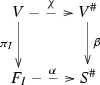
  commutes, that is, , where

  $$\begin{aligned} \pi _I:\prod \limits ^K_{i=1}F_i\rightarrow \prod \limits _{i\in I}F_i \end{aligned}$$

  is the natural projection onto a direct factor.

• (ii) Let $V^{\#}$ be a variety with ${\mathbb Q}$-factorial terminal singularities, satisfying the condition

  

  and $\chi :V\dashrightarrow V^{\#}$ a birational map. Then $\chi$ is a (biregular) isomorphism.

• (iii) The groups of birational and biregular self-maps of the variety V coincide:

  $$\begin{aligned} \mathrm{Bir}\,V=\mathrm{Aut}\,V. \end{aligned}$$

  In particular, the group $\mathrm{Bir}\,V$ is finite.

• (iv) The variety V admits no structures of a fibration into rationally connected varieties of dimension strictly smaller than . In particular, V admits no structures of a conic bundle or a fibration into rational surfaces.

• (v) The variety V is non-rational.

Since the inequality implies that and , Theorem 1.2 implies that generic complete intersections $F\in {\mathcal F}(\underline{d})$ with $\underline{d}\in {\mathcal D}_{\geqslant 8}$ for $|\underline{d}|\geqslant 3k+3$ satisfy the assumptions of Theorem 1.7.

1.4 The structure of the paper

In Sects. 2–3 we prove Theorem 1.6. We reproduce the proof sketched in [16, Section 3.1] in full detail, somewhat modifying the argument given in [16], adjusting it to a wider class of Fano complete intersections. In principle, the new argument is potentially applicable to proving the inequality for complete intersections $F\in {\mathcal F}(\underline{d})$ with $\underline{d}\not \in {\mathcal D}_{\geqslant 8}$.

Our main tool is the technique of hypertangent linear systems. This is a procedure (described in Sect. 3), the “input” of which is an effective divisor $D\sim nH_F$, such that the pair is not canonical (under the assumption that such pairs exist), and the “output” of which is an effective 1-cycle C that has a high multiplicity at some point $o\in F$. More precisely, if $\underline{d}\in {\mathcal D}_{\geqslant 8}$, then $\hbox {mult}_{o}\,C>{\hbox {deg}}\,C$, which is impossible. This contradiction proves Theorem 1.6.

In Sect. 4, we prove Theorem 1.5.

1.5 Historical remarks

As we pointed out above, the connection between the existence of Kähler–Einstein metrics and the global log canonical thresholds was established in [7, 12, 20]. The special importance of those papers is in that they connected some concepts of complex differential geometry with some objects of higher-dimensional birational geometry, which makes it possible to use the results of birational geometry to prove the existence of Kähler–Einstein metrics. That work was started in [1] and continued in [2,3,4,5,6, 8, 11, 16, 17]. Every time, a computation or estimate for the global log canonical threshold, obtained by the methods of birational geometry (the connectedness principle, inversion of adjunction, the technique of hypertangent divisors) yielded a proof of existence of Kähler–Einstein metrics for new classes of varieties. Such results are important by themselves, not speaking of their applications to birational geometry (Theorem 1.7), that is, of new classes of birationally rigid varieties.

2 Tangent divisors

In this section we start the proof of Theorem 1.6. We begin (Sect. 2.1) with some preparatory work: assuming that the pair is not canonical, we show the existence of a hyperplane section ${\Delta }$ of the variety F, such that the multiplicity of the restriction of the divisor D onto ${\Delta }$ at the point o is strictly higher than 2n. After that (Sect. 2.2) using the regularity condition (R), we construct a subvariety $Y\subset {\Delta }$ of codimension $k+1$ with a high multiplicity at the point o.

2.1 Inversion of adjunction

Assume that there exists an effective divisor such that the pair (F, (1 / n)D) is not canonical, that is, there is an exceptional divisor E over F, satisfying the Noether–Fano inequality

$$\begin{aligned} \mathrm{ord}_ED>na(E,F). \end{aligned}$$

By linearity of this inequality in the divisor D (the integer $n\in {\mathbb Z}_+$ depends linearly on D), we may assume that D is a prime divisor. Let $B\subset F$ be the centre of the exceptional divisor E. It is well known that the estimate

$$\begin{aligned} \mathrm{mult}_BD>n \end{aligned}$$

holds, whence by for example [16, Proposition 3.6], we immediately conclude that $\dim B\leqslant k-1$. Consider a point $o\in B$ of general position. Let be its blow up, the exceptional divisor. For some hyperplane ${\Theta }\subset E^+$ the inequality

holds, where $D^+$ is the strict transform of the divisor D on $F^+$ (see [16, Proposition 2.5] or [18, Chapter 7, Proposition 2.3]).

Now let us consider a general hyperplane section ${\Delta }$ of the complete intersection F, containing the point o and cutting out the hyperplane ${\Theta }$ on $E^+$ in the sense that . It is easy to see that the restriction of the divisor D on ${\Delta }$ satisfies the inequality

(2)

The hyperplane section ${\Delta }$ can be viewed as a complete intersection of the type $\underline{d}$ in ${\mathbb P}^{M+k-1}$.

2.2 Intersection with tangent hyperplanes

Now assume that F satisfies the condition (R). In the notations of Sect. 1.2 the system of linear equations

defines the (embedded) tangent space $T_oF\subset T_o{\mathbb P}$. Obviously, . Let $h(z_*)$ be the linear form, defining the hyperplane that cuts out ${\Delta }$. In particular,

and . Let

$i=1,\dots ,k$, be the tangent hyperplane sections of the variety ${\Delta }$. By the condition (R), the inequality $\dim {\Delta } \geqslant 2k+2$ and the Lefschetz theorem (taking into account that the singularities of the variety ${\Delta }$ are at most zero-dimensional and $o\in {\Delta }$ is a non-singular point), we may conclude that for any $j=1,\dots ,k$,

is an irreducible subvariety of codimension j in ${\Delta }$, which has multiplicity precisely $2^j$ at the point o. We will show that the effective divisor (where $H_{{\Delta }}$ is the class of a hyperplane section of the complete intersection ${\Delta }\subset {\mathbb P}^{M+k-1}$), satisfying inequality (2), cannot exist. Again by the linearity of inequality (2) (we will need no other information about the divisor ), we assume that is a prime divisor. In particular, inequality (2) implies that (since $\mathrm{mult}_oT_1=2$), so that the effective cycle of the scheme-theoretic intersection of these divisors is well defined and satisfies the inequality

$$\begin{aligned} \mathrm{mult}_oY^*_1>4n, \end{aligned}$$

and moreover, ; in particular,

where $d=\mathrm{deg}\,F=d_1,\dots , d_k$. In the sequel for simplicity of notations we write

$$\begin{aligned} \frac{\hbox {mult}_o}{\hbox {deg}} \end{aligned}$$

for the ratio of multiplicity at the point o to the degree. Let $Y_1$ be an irreducible component of the cycle $Y^*_1$ with the maximal value of $\mathrm{mult}_o/\mathrm{deg}$; in particular,

Since by construction $Y_1\subset T_1$ and

we conclude that $Y_1\not \subset T_2$ and the effective cycle is well defined and satisfies the inequality

Let $Y_2$ be an irreducible component of the cycle $Y^*_2$ with the maximal value of $\mathrm{mult}_o/\mathrm{deg}$.

Continuing in the same way, we construct a sequence of irreducible subvarieties

of codimension , satisfying the inequality

The inequality $M\geqslant 2k+3$ is needed to justify the last step in this construction: by the Lefschetz theorem, is an irreducible subvariety of ${\Delta }$ of codimension k, with the multiplicity $2^k$ at the point o and degree d, which makes it possible to form the effective cycle of codimension $k+1$.

We have shown the following claim.

Proposition 2.1

Assume that the pair is not canonical. Then for some point $o\in F$ and a hyperplane section ${\Delta }\ni o$, non-singular at the point o, there exists an irreducible subvariety $Y\subset {\Delta }$ of codimension $k+1$ in ${\Delta }$, satisfying the inequality

(3)

In order to complete the proof of Theorem 1.6, we now need the technique of hypertangent divisors. It is considered in the next section.

3 Hypertangent divisors

In this section we complete the proof of Theorem 1.6. First (Sect. 3.1) we construct hypertangent linear systems on the variety ${\Delta }$ and study their properties. After that (Sect. 3.2) we select a sequence of general divisors from the hypertangent systems. Finally, intersecting the subvariety Y with the hypertangent divisors, we complete the proof of Theorem 1.6 (Sect. 3.3).

3.1 Hypertangent linear systems

For let

$$\begin{aligned} f_{i,j}=q_{i,1}+\cdots +q_{i,j} \end{aligned}$$

be the truncated equation of the hypersurface $Q_i$. By the symbol ${\mathcal P}_{a, M+k}$ we denote the linear space of homogeneous polynomials of degree a in the coordinates $z_1,\dots ,z_{M+k}$. We use this symbol for $a<0$ as well, setting in that case .

Definition 3.1

The linear system of divisors

is the a-th hypertangent linear system on ${\Delta }$ at the point o.

Note that by our convention about the negative degrees only the polynomials $f_{i,j}$ of degree $j\leqslant a$ are really used in the construction of the system $\mathrm{\Lambda }_a$.

Set $\delta =d_k$ and for $a\geqslant 2$ set

Obviously, $k_a=0$ for $a\geqslant \delta +1$. The equality $d_1+\cdots +d_k=M+k$ implies that $\delta \leqslant M$. Obviously,

$$\begin{aligned} k=k_2+\cdots +k_{\delta }. \end{aligned}$$

We say that we are in

$$\begin{aligned} \begin{array}{ll} \textsc {Case I},&{}\quad \mathrm{if}\, k_{\delta }\geqslant 3,\\ \textsc {Case IIA},&{}\quad \mathrm{if}\, k_{\delta }=2,\\ \textsc {Case IIB},&{}\quad \mathrm{if}\, k_{\delta }=1\,\, \mathrm{and}\,\, k_{\delta -1}\geqslant 1,\\ \textsc {Case III},&{}\quad \mathrm{if}\, k_{\delta }=1\,\, \mathrm{and}\,\, k_{\delta -1}=0. \end{array} \end{aligned}$$

Obviously, one of these cases takes place: we simply listed all options.

For $a\geqslant 2$ set

$$\begin{aligned} m_a=\sum _{i\geqslant a}k_i. \end{aligned}$$

It is easy to see that $m_a$ is the number of polynomials of degree a in the sequence (1). In the next proposition we sum up the properties of hypertangent systems that we will need. The symbol $\mathrm{codim}_o$ stands for the codimension in a neighborhood of the point o with respect to ${\Delta }$.

Proposition 3.2

• (i) The following inclusion holds: , where $H_{{\Delta }}$ is the class of a hyperplane section of ${\Delta }$.

• (ii) The following equality holds: $\mathrm{mult}_o\mathrm{\Lambda }_a=a+1$.

• (iii) In Cases I and IIA for $a=1,\dots ,\delta -2$, and in Cases IIB and III for $a=1,\dots ,\delta -3$ the following equality holds:

  

• (iv) In Case I for $a=\delta -1$, in Cases IIA and IIB for $a=\delta -2$, and in Case III for $a=\delta -3$ the following equality holds: $\dim \mathrm{Bs}{\Lambda }_{a}=1$.

Note that (iii) in Case IIA for $a=\delta -2$ and in Case III for $a=\delta -3$ coincides with (iv) for these cases.

Proof

These are the standard facts of the technique of hypertangent divisors, following immediately from the regularity condition (Definition 1.4), see [18, Chapter 3]. Claim (i) is obvious, claim (ii) follows from the equality

(4)

where the dots stand for the components of degree $j+2$ and higher, and from the regularity condition. Claims (iii) and (iv) follow from equality (4) and the counting of polynomials of degree j in the sequence (1). For the details, see [18, Chapter 3]. $\square$

3.2 Hypertangent divisors

The next step is constructing a sequence of hypertangent divisors . From each hypertangent linear system $\mathrm{\Lambda }_i$ we select $l_i$ divisors, where the integer $l_i$ is defined in the following way: $l_2=m_3-1$, $l_i=m_{i+1}$ for $i=3,\dots ,\delta -3$, finally,

• in Case I, $l_{\delta -2}=m_{\delta -1}$, $l_{\delta -1}=m_{\delta }-2$,

• in Case IIA, $l_{\delta -2}=m_{\delta -1}$,

• in Case IIB, $l_{\delta -2}=m_{\delta -1}-1$.

For all other values of i set $l_i=0$.

Furthermore, for $l_i\ne 0$ we set

and a tuple of divisors $(D_{i,1},\dots ,D_{i,l_i})\in {\mathcal L}_i$ is denoted by the symbol $D_{i,*}$. Finally, set

$$\begin{aligned} {\mathcal L}=\prod _{i\geqslant 2}{\mathcal L}_i, \end{aligned}$$

where the direct product is taken over all i such that $l_i\ne 0$, see the definition of the integers $l_i$ above. It is easy to see that ${\mathcal L}$ is the direct product of

$$\begin{aligned} \sum _{i\geqslant 2}l_i=M-k-3 \end{aligned}$$

factors (precisely the number of polynomials in the sequence (1), from which all linear and quadratic forms are removed, together with one cubic polynomial and the last two polynomials). The elements of of the space ${\mathcal L}$, that is, the tuples of divisors

$$\begin{aligned} (D_{2,*},D_{3,*},\dots ) \end{aligned}$$

are denoted by the symbol $D_{*,*}$.

For an arbitrary equidimensional effective cycle W on ${\Delta },\dim W\geqslant 2$, and a divisor , such that none of the components of W is contained in its support $|D_{i,j}|$, we denote by the symbol

the effective cycle of dimension $\dim W-1$, which is obtained from the cycle of the scheme-theoretic intersection of W and $D_{i,j}$ (see [10, Chapter 2]) by removing all irreducible components, not containing the point o.

3.3 Proof of Theorem 1.6

Now everything is ready to apply the technique of hypertangent systems to the subvariety $Y\subset {\Delta }$, constructed in Sect. 2. The tuple is understood as a tuple of divisors

$$\begin{aligned} (D_{2,1},D_{2,2,},\dots ,D_{3,1},\dots ), \end{aligned}$$

which makes it possible to apply the construction of the scheme-theoretic intersection at the point o, described above, many times.

Proposition 3.3

For a general tuple the effective 1-cycle

is well defined and satisfies the inequalities

and

Proof

The procedure of constructing the cycle C is justified by Proposition 3.2 (iii)–(iv), and the inequalities for the degree and multiplicity follow from claims (i) and (ii). $\square$

Let us prove Theorem 1.6. Assume that . Combining inequality (3) with inequalities of Proposition 3.3, we obtain the estimate

and after cancellations we see that the inequality $\mathrm{mult}_oC>\mathrm{deg}\,C$ holds. (For the details, see [16, Section 3].) This contradiction completes the proof of Theorem 1.6.

4 Regular complete intersections

In this section we prove Theorem 1.5. First (Sect. 4.1), we reduce the problem to a local problem about violation of the regularity condition at a fixed point. After that (Sect. 4.2), we estimate the codimension of the set of tuples of polynomials, vanishing simultaneously on some line. Finally (Sect. 4.3), we estimate the codimension of the set of tuples of polynomials, the set of common zeros of which has an “incorrect” dimension, but is not a line. This completes the proof of Theorem 1.5.

4.1 Reduction to the local problem

Following the standard scheme of proving the regularity conditions (see [18, Chapter 3] or any paper that makes use of the technique of hypertangent divisors, for example, [14] or [8]), we have to show that a violation of the local regularity condition at a fixed point o (that is, Definition 1.4 (i)) imposes at least $M+1$ independent conditions on the coefficients of the polynomials (1). The complete intersection F is non-singular, so let us fix the linear forms $q_{1,1},\dots ,q_{k,1}$ and so the linear space

The last two polynomials in the sequence (1) are not used in the regularity condition. Let us re-label the polynomials of the sequence (1), from which all linear forms and the last two polynomials are removed, by the symbols

$$\begin{aligned} p_1,\;\;\dots ,\;\;p_{M-2}. \end{aligned}$$

Now the local regularity condition can be stated as follows: for any hyperplane $S\subset T_oF$ (in the notations of Definition 1.4, ) the sequence

$$\begin{aligned} p_1|_S,\;\;\dots ,\;\;p_{M-2}|_S \end{aligned}$$

is regular at the origin. If ${\mathbb S}={\mathbb P}(S)\cong {\mathbb P}^{M-2}$, then this means that the closed subset

is zero-dimensional. Fix an isomorphism $T_oF\cong {\mathbb C}^M$. Set and ${\mathbb T}={\mathbb P}(T_oF)\cong {\mathbb P}^{M-1}$. Let ${\mathcal P}_{a,M}$ be the space of homogeneous polynomials of degree a on ${\mathbb C}^M$ (or ${\mathbb P}^{M-1}$) and

$$\begin{aligned} {\mathcal P}_{\mathbb T}=\prod ^{M-2}_{i=1}{\mathcal P}_{\delta (i),M}. \end{aligned}$$

If all polynomials $p_i$ vanish on a line $L\subset {\mathbb T}$, then, obviously, the local regularity condition is violated: it is sufficient to take any hyperplane ${\mathbb S}\supset L$. For that reason the case when the set contains a line will be considered separately.

4.2 The case of a line

Let be a closed subset of tuples $(p_1,\dots ,p_{M-2})$, such that for some line $L\subset {\mathbb T}$,

$$\begin{aligned} p_1|_L\equiv \cdots \equiv p_{M-2}|_L\equiv 0. \end{aligned}$$

Proposition 4.1

The following inequality holds: .

Proof

The proof is obtained by elementary but not quite trivial computations.

Lemma 4.2

The following inequality holds:

Proof

The first component in the right hand side is the codimension of the set of tuples of polynomials vanishing on a fixed line $L\subset {\mathbb T}$. Subtracting the dimension of the Grassmanian of lines, we complete the proof. $\blacksquare$

Considering the polynomials $q_{i,j}$ for each $i=1,\dots ,k$ separately, we conclude that

where for $i=1,\dots ,k-2$, in Cases I and IIA and , in Cases IIB and III. In any case and

$$\begin{aligned} a_1+\cdots +a_k=M+k-2. \end{aligned}$$

Lemma 4.3

The minimum of the quadratic function

on the set of integral vectors such that all and $a_1+\cdots +a_k=A$, where $A=ka+l$, $a\in {\mathbb Z}$ and , is equal to

Proof

Without loss of generality we assume that the set is ordered: $a_i\leqslant a_{i+1}$. It is easy to check that if two positive integers u, v satisfy the inequality $u\leqslant v-2$, then

Therefore, if , then, replacing the vector by the vector , where for $j\ne i,i+1$, and , we decrease the value of the function $\xi$. Similarly, if

then, replacing the vector $\underline{a}$ by the vector $\underline{a}'$ with

we decrease the value of the function $\xi$. In both cases the vector $\underline{a}'$ remains ordered and satisfies the restrictions $a'_1+\cdots +a'_k=A$, . Since the set of such vectors is finite, applying finitely many modifications of the two types described above, we obtain a vector with

which realizes the minimum of the function $\xi$. Simple computations complete the proof of the lemma. $\blacksquare$

Now writing $M-2=ka+l$ with and applying Lemmas 4.2 and 4.3, after obvious simplifications we obtain the inequality

Now the inequality of Proposition 4.1 follows from the estimate

which is easy to check (recall that by assumption $M\geqslant 2k+3$, so that $ak+l\geqslant 2k+1$ and, in particular, $a\geqslant 2$). $\square$

Starting from this moment, we assume that the polynomials $p_1,\dots ,p_{M-2}$ do not vanish simultaneously on a line $L\subset {\mathbb T}$.

4.3 End of the proof of Theorem 1.5

Fix a hyperplane ${\mathbb S}\subset {\mathbb T}$ and its isomorphism ${\mathbb S}\cong {\mathbb P}^{M-2}$. Set

$$\begin{aligned} {\mathcal P}=\prod ^{M-2}_{i=1}{\mathcal P}_{\delta (i),M-1}. \end{aligned}$$

Since the hyperplane ${\mathbb S}$ varies in an -dimensional family, it is sufficient to show that the codimension of the set of tuples $(p_1,\dots ,p_{M-2})\in {\mathcal P}$ such that the closed set

has a component of positive dimension, which is not a line, is of codimension at least $(M+1)+(M-1)=2M$ in ${\mathcal P}$. Let us check this fact. The check is not difficult, arguments of that type were published many times in full detail, so we will just sketch the main steps.

Let be the set of such tuples that the closed set

(5)

(if $i=0$, then this set is assumed to be equal to ${\mathbb P}^{M-2}$) is of codimension $i-1$ in ${\mathbb P}^{M-2}$, but for some irreducible component B of this set we have $p_i|_B\equiv 0$, and moreover if $i=M-2$, then B is a curve of degree at least two.

Obviously, Theorem 1.5 is implied by the following fact.

Proposition 4.4

The following inequality holds:

Proof

Using the method that was applied in [13] (see also [18, Chapter 3, Subsection 1.3]), for $i=1,\dots ,k$ we obtain the estimate

(recall that for $i=1,\dots ,k$). The minimum of the right hand side is attained at $i=k$ and it is easy to check that

Therefore, we may assume that $i\geqslant k+1$, so that . Now we use the technique that was developed in [14] (see also [18, Chapter 3, Section 3]). Let be the set of tuples such that the closed set (5) is of codimension $i-1$, and moreover, there is an irreducible component B of this set, such that

, $b\ne M-3$, and $p_i|_B\equiv 0$. Since

(the condition $b\ne M-3$ for $i=M-2$ is meant, but not shown, in order for the formula not to be ugly), it is sufficient to show the inequality

for $i\geqslant k+1$, , $b\ne M-3$.

Now the technique of good sequences and associated subvarieties, which we do not give here, see [14] or [18, Chapter 3, Section 3], gives the estimate (taking into account the dimension of the Grassmanian of linear subspaces of codimension b in ${\mathbb P}^{M-2}$)

The right hand side of this inequality, considered as a function on the set , can decrease or increase or first increase and then decrease. In any case the minimum of the right hand side is attained either at $b=0$ (and equals $3M-5\geqslant 2M$), or at $b=i-1$ (if $i\leqslant M-3$) or $b=M-4$ (if $i=M-2$), when it is also not smaller than 2M. $\square$

References

Cheltsov, I.A.: Log canonical thresholds on hypersurfaces. Sb. Math. 192(7–8), 1241–1257 (2001)
Cheltsov, I.A.: Extremal metrics on two Fano manifolds. Sb. Math. 200(1–2), 95–132 (2009)
Cheltsov, I.A.: Log canonical thresholds of Fano threefold hypersurfaces. Izv. Math. 73(4), 727–795 (2009)
Cheltsov, I.A., Park, J.: Global log-canonical thresholds and generalized Eckardt points. Sb. Math. 193(5–6), 779–789 (2002)
Cheltsov, I., Park, J., Won, J.: Log canonical thresholds of certain Fano hypersurfaces. Math. Z. 276(1–2), 51–79 (2014)
Cheltsov, I.A., Shramov, K.A.: Log canonical thresholds of smooth Fano threefolds. Russian Math. Surveys 63(5), 859–958 (2008)
Demailly, J.-P., Kollár, J.: Semi-continuity of complex singularity exponents and Kähler–Einstein metrics on Fano orbifolds. Ann. Sci. Éc. Norm. Supér. 34(4), 525–556 (2001)
Eckl, T., Pukhlikov, A.V.: On the global log canonical threshold of Fano complete intersections. Eur. J. Math. 2(1), 291–303 (2016)
Fujita, K.: K-stability of Fano manifolds with not small alpha invariants (2016). arXiv:1606.08261
Fulton, W.: Intersection Theory. Ergebnisse der Mathematik und ihrer Grenzgebiete, vol. 2. Springer, Berlin (1984)
Kim, I.-K., Okada, T., Won, J.: Alpha invariants of birationally rigid Fano threefolds (2016). arXiv:1604.00252
Nadel, A.M.: Multiplier ideal sheaves and Kähler–Einstein metrics of positive scalar curvature. Ann. Math. 132(3), 549–596 (1990)
Pukhlikov, A.V.: Birational automorphisms of Fano hypersurfaces. Invent. Math. 134(2), 401–426 (1998)
Pukhlikov, A.V.: Birationally rigid Fano complete intersections. J. Reine Angew. Math. 541, 55–79 (2001)
Pukhlikov, A.V.: Birational geometry of Fano direct products. Izv. Math. 69(6), 1225–1255 (2005)
Pukhlikov, A.V.: Birational geometry of algebraic varieties with a pencil of Fano complete intersections. Manuscripta Math. 121(4), 491–526 (2006)
Pukhlikov, A.V.: Existence of the Kähler–Einstein metric on certain Fano complete intersections. Math. Notes 88(3–4), 552–558 (2010)
Pukhlikov, A.: Birationally Rigid Varieties. Mathematical Surveys and Monographs, vol. 190. American Mathematical Society, Providence (2013)
Pukhlikov, A.V.: Birationally rigid complete intersections of quadrics and cubics. Izv. Math. 77(4), 795–845 (2013)
Tian, G.: On Kähler–Einstein metrics on certain Kähler manifolds with \(C_1(M)>0\). Invent. Math. 89(2), 225–246 (1987)
Acknowledgements
Various technical points, related to the constructions of the present paper, were discussed by the author in his talks given in 2009–2016 at Steklov Mathematical Institute. The author thanks the members of Divisions of Algebraic Geometry and of Algebra and Number Theory for the interest to his work. The author also thanks his colleagues in the Algebraic Geometry research group at the University of Liverpool for the creative atmosphere and general support.
The author is grateful to the referee for a number of useful comments.
Author information
Authors and Affiliations
Corresponding author
Rights and permissions
Open Access This article is distributed under the terms of the Creative Commons Attribution 4.0 International License (http://creativecommons.org/licenses/by/4.0/), which permits unrestricted use, distribution, and reproduction in any medium, provided you give appropriate credit to the original author(s) and the source, provide a link to the Creative Commons license, and indicate if changes were made.
About this article
Cite this article
Pukhlikov, A.V. Canonical and log canonical thresholds of Fano complete intersections. European Journal of Mathematics 4, 381–398 (2018). https://doi.org/10.1007/s40879-017-0152-6
Received:
Accepted:
Published:
Issue Date:
DOI: https://doi.org/10.1007/s40879-017-0152-6