Maximum power point tracking of the solar power plants in shadow mode through artificial neural network

Abstract

The use of solar cells despite being free of contamination and unlimited in terms of the amount of energy is considered as a costly way to generate energy. Two main factors may be enumerated as follows. First of all, the amount of sunlight and ambient temperature affected the amount of energy received from sunlight by solar panels, as long as the amount of sunlight changes overnight in line with changing weather conditions and the second one is the low efficiency of the energy conversion. The main reason for the low electrical efficiency is the nonlinear variation of the output voltage and current along with the change of the amount of radiation, the change of the temperature of the operating environment and the change of the electric charge, respectively. To address this concern, the maximum point of the photovoltaic system can be tracked through an appropriate algorithm and pushes the system point to the optimal point. In a word, the key goal of the investigation presented here is to provide an approach that in the high speed and precision of convergence to the maximum power point is well considered. So far, a large number of available methods have been used to increase the efficiency of solar cells. Some of these are associated with problems in the tracking process or they respond slowly. It should be noted that a set of them are depended on the types and structures of solar cells and also their implementation is very complex and costly. Therefore, this study has focused on intelligence-based techniques such as artificial neural networks to solve all the problems mentioned. The investigated outcomes verify the effectiveness of the approach performance proposed.

Introduction

The renewable resources have attracted the much more attention of scholars due to increasing demand for energy, increasing fuel prices, increasing global warming, and paying attention to environmental pollution. Many sources are available as renewable energies, such as solar energy, wind, geothermal, hydrogen (fuel cell), and so on. But it seems that the tendency toward more solar energy is more among them [1]. The photovoltaic (PV) systems do not emit any pollution environmentally and produce no noise, they also do not require fuel for fuel economically, they need little maintenance, and most importantly, they are interminable. Only 1 h of solar-to-earth energy means 1 year’s energy consumption for the whole world. Therefore, these systems can be used on large scale [2]. In Germany only in 2010, 7.4 GW of solar energy (1.4 of the total capacity of the entire Iran electricity grid), or in other words, more than 30 million solar arrays are installed. The total installed capacity in Germany, Spain, Japan, Italy, and the United States was 17.3, 7.7, 3.6, 3.5, and 2.5 GW, respectively, while the radiant intensity of the sun in Germany and Japan is about half of Iran. The cost of the PV power generation systems has significantly declined over the past 20 years, has reached from 25 dollars per kilowatt in the 1980s to 2 dollars per kilowatt in 2010 [3]. The PV systems in network-independent mode have been widely used in water pumps, street lighting, home use, battery of chargers, and satellites to be used in hybrid and power systems in network-connected mode. Today, these applications have dedicated themselves only 0.5% of the world’s energy consumption and are projected until the year 2050, this amount may reach about 45%. According to the World Energy Agency report of the European countries in the joint project until 2050, they plan to use solar energy from the region to supply electricity to Europe by installing PV modules in the Africa’s Great Desert. Studies show that only 0.3% of this energy may be enough to meet the European electricity requirements [4]. The PV systems have two major disadvantages:

• High cost and very low efficiency (about 9–16%);

• Continuous changes in the amount of power produced by atmospheric conditions (the temperature and the radiation).

Many works have been done in the field of modeling and controlling PV cells. The study of maximum power point tracking techniques to use in the partial shadow conditions (PSC) is part of these works. The PSC conditions often occur in large PV power generation systems. It causes loss of system power output, the effects of hot spots, and safety and reliability problems. As long as the PSC occurs, the power–voltage characteristic curve shows several peak value, because this curve represents a general maximum power point and several local maximum power points. Regarding the materials presented in [5], it contains various information from the general maximum power point tracking (MPPT) algorithms and the appropriate hardware design for the PSC. Based on the electrical characteristics, the PV cell modeled in the study is equivalent to a diode. This model includes an current source $I_{\text{S}}$, a diode current $I_{\text{d}}$, a parallel equivalent resistance $R_{\text{P}}$, and an equivalent series resistance $R_{\text{S}}$. The output current of the PV module, $I_{\text{PV}}$, is different between the current generated by the light $I_{\text{S}}$ and the diode current $I_{\text{d}}$. That research includes several algorithms and hardware architectures related to solving the PSC problems that collects, classifies and compares the new MPPT techniques from a variety of references. Finally, the MATLAB software has been widely used to simulate the five common MPPT algorithms and detect its tracking performance. According to the simulation results, agent system-based MPPT methods can still be improved in terms of accuracy of tracking.

In Ref. [6], analysis and enhancement of the photovoltaic cell efficiency by the MPPT incremental conductance method under nonlinear loading conditions has been investigated. This research presents experimental tests for types of energy efficiency obtained from a photovoltaic unit under nonlinear loading in combination with the MPPT incremental conductance algorithm. The focus of that study was to evaluate the photovoltaic panel under nonlinear load conditions using an experimental setup of a photovoltaic array connected to a DC–AC converter and KVA inverter that produced a nonlinear load. In nonlinear loading conditions, both the simulation and the experiment showed that the MPPT method does not reach the maximum power point due to the waves in the current and eventually leads to a reduction in productivity. In that study, the panel current is applied as a function of the load apparent resistance in the MPPT algorithm to eliminate the power change by varying the apparent resistance of the load and providing the voltage under the nonlinear conditions. This system was simulated using the Simulink MATLAB software for nonlinear loads. A TMDSSOLAREXPKIT was used to control the MPPT. In the second case, the inverter was connected to a single-phase network. When a voltage increase occurs in the network, photovoltaic power falls. This power reduction is reduced using the proposed MPPT method.

In Ref. [7], a review of different methods of tracing the maximum power point in photovoltaic systems has been made. The PV power in electrical power generation is constantly increasing. The MPPT tracking in the PV systems presents an important work and a challenge issue. In the MPPT method, the DC–DC converter is set to be the maximum power obtained from the PV system. In that study, the existing MPPT strategies such as classical one (including perturb and observe, incremental conductance, current sweep and constant voltage method) and the modern MPPT methods (including the MPPT-based artificial intelligence network ANN, the MPPT-based fuzzy controller FLC, the MPPT-based metaheuristic algorithms).

In Ref. [8], the methods of maximum power point tracking of the PV system for a uniform sunshine and partial shadowing conditions are investigated. For this purpose, it examines the most advanced MPPT methods in the PV power system. The main methods to be examined are: observation and tracking, incremental conductance and hill climbing. In addition, adaptive variation of these methods is considered. Furthermore, the most recent MPPT techniques using soft computing methods such as fuzzy logic control, artificial neural networks and evolutionary algorithms are included in that study. That research also provides a detailed operation for the MPPT in the uniform sunshine process and its focus is on the application of the above methods in partial shading conditions.

In Ref. [9], the MPPT control scheme is presented with the help of intelligent neural network algorithm based on a inverter controlled by hysteresis current for photovoltaic systems. These days, the photovoltaic panel is one of the most important sources of renewable energy. This panel can use DC power directly in the related applications. In the daily life, it generally works with AC loads. The proposed inverter in that study has a robust performance and easy operation capability. The controlled inverter with fixed-banded hysteresis has been determined and the load variations with the THD output current are set to be less than 5%. The inverter is developed by the three-level technique. The MPPT is designed through the artificial neural network. In that study, the feeding of AC systems by solar power is analyzed in isolation mode and the results are obtained. The results indicate that the artificial neural network method has very satisfactory results with an efficiency of 99%.

In Ref. [10], the original and accurate simulation of the photovoltaic system is proposed based on the seven-parametric model. The output characteristics of the photovoltaic array are highly nonlinear. Therefore, the study and analysis of the performance of the PV system in the changing environmental conditions requires an efficient and accurate model for the PV. The proposed simulator can produce accurate specifications of the output of the PV system under different operating conditions. Also, this simulator is flexible enough and can simulate different combinations of the PV panels with parallel/serial connections. The power of the proposed simulator is shown under the conditions of a partial shadow. Moreover, the performance of the developed simulator has been confirmed by connecting it to the actual power electronic converter and the maximum power point controller. The proposed PV simulator should facilitate different aspects of the design of the PV systems and be very useful in assessing the behavior of newly developed controllers before their practical implementation.

In this study, first, the problem caused due to the presence of several local maximum points on the multi-dimensional array P–I characteristic curve is explained. The main problem investigated is designing a new method for the performance of two arrays with series connection at their maximum point. In this study, a new method provided to maximize power is presented in two steps, which, by ignoring local maxima, if any, the maximum location is determined. The first step includes a search algorithm that determines the location of approximate performance point near the general maximum power point and uses it as the starting point of the second stage. The first step is repeated if the temperature changes or radiation of the PV array is increased by 30%, which is obtained by trial and error. The second step can be any maximum tracking method. In this study, P and O and RCC methods are used. The tracking efficiency was about 95% using two methods and the convergence time under varying atmospheric conditions was 15 Ms. Innovation of the proposed method is to use a search algorithm that receives the power and current of the PV array, and general maximum is estimated in its output. This algorithm improves the capability of existing one-step methods and increases their efficiency [11,12,13,14,15,16,17,18,19,20,21,22].

The rest of the paper is organized as follows: “The preliminary of components”, “The proposed control approach” is discussed. “The simulations” and “Conclusion” are finally addressed.

The preliminary of components

The orbital model of photovoltaic cell

The PV cells have a nonlinear I–V characteristic that depends on the amount of sun radiation and cell temperature. Under ideal conditions, a solar cell can be modeled by current source that is parallel to a diode. However, the losses caused by these cells are modeled by $R_{\text{S}}$ as the series resistance and the $R_{\text{SH}}$ as the parallel resistance. Therefore, in real conditions, the orbital model of the PV cell is shown in Fig. 1. The value of $R_{\text{S}}$ is usually low, small and the $R_{\text{SH}}$ value is very high. Also, the current of the Iph source is set to zero in the dark conditions [1, 2].

Fig. 1

The PV cell circuit model

The PV module

The resistance in the equivalent circuit defines the losses in the cell. The losses in the affected cell are the cases such as the reflection of sunlight at the cell surface, the absorption of photons without the creation of electrons and free holes, the redistribution of electrons and voids, and such related cases. According to Fig. 1, the solar cell’s characteristic equation is expressed by the following equation [11].

$$ I_{\text{pv}} = I_{\text{ph}} - I_{\text{D}} - I_{\text{SH}} , $$

(1)

where $I_{\text{pv}}$ is the current PV; $I_{\text{D}}$ is the diode’s current; $I_{\text{SH}} = \frac{{V_{\text{pv}} + I_{\text{pv}} R_{\text{S}} }}{{R_{\text{SH}} }}$ is the leakage current; $V_{\text{pv}}$ and $I_{\text{pv}}$, are the voltage and output current, respectively; $R_{\text{S}}$ and $R_{\text{SH}}$ are the equivalent series and parallel resistance of the solar cell. The diode current $I_{\text{D}}$ according to the voltage–current characteristic of the Shockley diode is expressed in the following relation.

$$ I_{\text{D}} = I_{\text{o}} \left( {{\text{e}}^{{\frac{{V_{\text{D}} }}{{aV_{\text{t}} }}}} - 1} \right). $$

(2)

Here, $I_{\text{o}}$ is the reverse saturation current; $V_{\text{D}} = V_{\text{pv}} + I_{\text{pv}} R_{\text{S}}$ is the diode voltage; $a$ is the diode ideal constant; $V_{\text{t}} = \frac{{N_{\text{s}} \cdot k_{\text{b}} }}{e}T$ is the diode thermal voltage; $N_{\text{s}}$ is the number of series cells; $k_{\text{b}}$ is the Boltzmann constant; $e$ is the charge of an electron and finally $T$ is the solar cell temperature. With the insertion of Eq. (2) into (1), the characteristic equation of a solar panel is obtained as:

$$ I_{\text{pv}} = I_{\text{ph}} - I_{\text{o}} \left( {{\text{e}}^{{\frac{{v_{\text{pv}} + I_{\text{pv}} R_{\text{S}} }}{{aV_{\text{t}} }}}} - 1} \right) - \frac{{v_{\text{pv}} + I_{\text{pv}} R_{\text{S}} }}{{R_{\text{SH}} }}. $$

(3)

In Eq. (3), the value of photovoltaic current $I_{\text{pv}}$, with the change of the intensity of light and temperature changes the following relation.

$$ I_{\text{pv}} = \left[ {I_{{{\text{pv}} \cdot {\text{ref}}}} + K_{\text{I}} \left( {T - T_{n} } \right)} \right]\frac{G}{{G_{n} }}, $$

(4)

where $I_{{{\text{pv}} \cdot {\text{ref}}}}$ is the PV current in the standard conditions; $K_{\text{I}}$ is the coefficient ratio of short-circuit current to the temperature in the standard conditions and $G$ is the light intensity.

$G_{n} = 1000\frac{W}{{m^{2} }}$ and temperature $T_{n} = 25\,^{ \circ } {\text{C}}$ are the standard test conditions of the solar cell. In Eq. (4), since the value of $R_{\text{SH}}$ is very high, the fraction of $\frac{{v_{\text{pv}} + I_{\text{pv}} R_{\text{S}} }}{{R_{\text{SH}} }}$ approaches the zero. Therefore, in a good approximation, the equation above is converted to the following equation [12]:

$$ I_{\text{pv}} = I_{\text{ph}} I_{\text{o}} \left( {{\text{e}}^{{\frac{{q \left( {v_{\text{pv}}\,+\,I_{\text{pv}} R_{\text{S}} } \right)}}{{N_{\text{s}} \cdot A \cdot K \cdot T}}}} - 1} \right). $$

(5)

Equation (5) is called the current equation of the solar cell. Thus, if the PV module contains the Np series cells and the $R_{\text{SH}}$ resistance is infinity, the equations related to the voltage, the current, and the power are obtained, respectively, by Eqs. (6), (7), and (8), respectively.

$$ V_{\text{pv}} = \left( {\frac{{N_{\text{s}} \cdot A \cdot K \cdot T}}{q}} \right) \cdot \ln \left( {\frac{{N_{\text{p}} \cdot I_{\text{ph}} - I_{\text{pv}} + N_{\text{p}} \cdot I_{\text{o}} }}{{I_{\text{o}} }}} \right) - R_{\text{S}} I_{\text{pv}} , $$

(6)

$$ I_{\text{pv}} = N_{\text{p}} \cdot I_{\text{ph}} - N_{\text{p}} \cdot I_{\text{o}} \left( {{\text{e}}^{{\frac{{q \left( {v_{\text{pv}} + I_{\text{pv}} R_{\text{S}} } \right)}}{{N_{\text{s}} \cdot A \cdot K \cdot T}}}} - 1} \right), $$

(7)

$$ p_{\text{pv}} = V_{\text{pv}} I_{\text{pv}} . $$

(8)

In the above relations, $I_{0}$ is the reverse saturation current value, with changes in temperature, by the following

$$ I_{0} = I_{{0 \cdot {\text{ref}}}} \left( {\frac{T}{{T_{n} }}} \right)^{3} { \exp }\left[ {\frac{{{\text{e}} \cdot E_{\text{g}} }}{{k_{\text{b}} \cdot a \cdot V_{\text{t}} }}\left( {\frac{1}{{T_{n} }} - \frac{1}{T}} \right)} \right]. $$

(9)

Here, $I_{{0 \cdot {\text{ref}}}}$ is the reverse saturation current in the standard conditions and $E_{\text{g}} = 1.121\left[ {1 - 0.0002677\left( {T - T_{n} } \right)} \right]$ is the distance of the power strips of silicon at 1 eV. Other variables of the above equations are tabulated in Table 1 [15].

Table 1 Variables of the PV cell

The characteristics curve of the PV module

The characteristics curve of the PV module is I–V, P–V and P–V curves that are dependent on the voltage, the current, and the power of the PV array. Figure 2 shows I–V, P–V and P–V curves. According to this figure, the bending point of the I–V, P–V, and P–V curves is a Maximum Power Point (MPP) at the specific temperature and the radiation (where the temperature is taken as 25 °C and the radiation is taken as 100 W/m²). When the PV module operates at this point, the maximum power from the module is received and the module has the maximum efficiency. The MPP is also known as general maximum [16].

Fig. 2

The P–I, I–V and P–V characteristics curve of the PV modulus

Factors affecting the performance of the modules and their characteristic curves

The characteristics of the PV module depend on the cell temperature, the sun radiation level, and so on. Some of these factors, such as the temperature and the irradiation, change may be made continuously throughout the day, and as a result, the characteristics of the cell change. We should briefly examine these factors [17]:

• (A) Temperature: an increase in temperature decreases the voltage and the current that is almost constant as shown in Fig. 3.

  Fig. 3

  

  Changes of the PV array curves or temperature at constant radiation intensity

• (B) The intensity of the sun radiation: the increase in the intensity of the radiation increases the current and the voltage that is almost constant as shown in Fig. 4.

  Fig. 4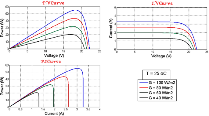

  

  Changes of the PV array curves or the radiation intensity at constant temperature

• (C) Array structure: the performance of the array depends on the type of cells used and the quality of manufacturing by the manufacturer. The values of $R_{\text{SH}}$ and $R_{\text{S}}$ can vary with respect to the structure. The value of $R_{\text{SH}}$ approaches the infinite and the value of $R_{\text{S}}$ approaches the zero in a high-quality cell.

• (D) Shadows: there are complete or incomplete shadows, which are often created by passing clouds, the adjacent buildings and the towers, the trees, the electricity and the telecommunication stands, and so on. In the penumbra conditions, several local maximum points—in addition to the general maximum—are created, and therefore, the characteristics of the PV array are complex. This makes it more difficult to track maximum point.

Description of the problem

In general, two factors cause the penumbra formation [18, 19, 20], including:

• Creating a shadow by the adjacent the buildings and the towers, the trees, the power towers, the telecommunications and etc. on the PV array in urban areas.

• Change in the angle of the radiation during a day or a season or passing clouds.

Now, the problem is described as follows: If two modules are connected in a series of the PV array and only one of the modules is affected (the penumbra conditions), then the I–V, P–I and P–V curves are affected by this penumbra. Figure 5 shows the I–V curve of the PV array under the penumbra conditions.

Fig. 5

The PV array curve or series connection under the penumbra conditions

It is observed that the above array has a local maximum point in addition to a general maximum under the penumbra conditions and since the goal is the maximum point tracking, this can make tracking more difficult [21]. The significant drop in the power received from the PV array due to shadow has caused designers to consider the smallest possible shadow to select the right place for creating the PV farm. It should also be noted that the penumbra is associated with the temperature drop. So, in short, we can say that the shadow creates one or more local maximums, in addition to general maximum, and this causes the maximum power point tracking problem to make mistakes sometimes. Since the goal is to determine the maximum general point, there are several algorithms for this purpose, which are discussed in the next section of the proposed control approach.

The proposed control approach

To discuss the proposed control approach, it is first essential to note that the shadow on the two modules having the series of connection creates a local maximum and a general maximum. The maximum local tracking instead of the general maximum leads to decrease the power, significantly. The method presented in this study provides a two-stage maximum power tracking method that determines the maximum point for two modules having serial connection. In the first step, the radiation and the temperature of the array is measured and the final P–I curve is found. Then, a search algorithm is implemented to approximate the MPP location with two current and power parameters at the MPP point. When the weather conditions exceed beyond a certain level, the search is repeated. In the second step, the actual characteristic curve starts the search for MPP from the estimated point in the first stage or from its previous performance point, which depends on changes in the performance conditions. Each of the MPPT single-step methods introduced in the previous section can be used in the second stage. As mentioned earlier, the second phase of this approach is performed using P and O and RCC methods, and this investigation uses the artificial neural network. In one such case, P and O and RCC methods are used to perform the second phase of this algorithm, and the neural network is realized, correspondingly.

The first step

As long as each module of the PV array has the certain change in ΔG and ΔT, the corresponding P–I curve is formed and the search algorithm is carried out to find both the local and general maximum. If there are both maximums, the general maximum is determined by the controller. The amount of changes in ΔG and ΔT throughout the day is not constant due to their different changes pattern. Therefore, the approximated value of these changes causes the controller to form a new P–I curve and begin a new search, which should be determined during the simulations of the system. The idea of providing the search algorithm can be useful when it does not call on a regular basis. This position may occur in an environment with rapid meteorological conditions (less than one second) to find the maximum point that should be difficult. Obviously, this search algorithm can be a solution to find the maximum of a function. But the search algorithm is provided as the starting point in the second stage, so it is not always online except in two modes: one at the start of the simulation that runs once and the other is the high variations of ΔG and ΔT from a given limit.

The second step

This second step, which is performed using a two-layer feed-forward neural network, uses the estimated MPP point in the first stage as the starting point for determining and tracking general maximum. This is expected that this starting point help excludes any undesirable local maximum. At this step, the neural network initially receives power changes to the voltage of the PV array. When the power value is constant, the voltage must remain unchanged. But as long as the amount of power increases or decreases, the array voltage must also be changed proportional to the power to reach the maximum power point. The neural network has many advantages, such as high performance accuracy and very good convergence speed. On the other hand, this algorithm, unlike the many MPPT methods, does not oscillate around the MPP point. In cases where natural disturbances are created due to switching converter circuits, these oscillations should not be more affected by disturbances of the converter and the voltage of the array. As mentioned in the previous section of this research, in the boost converters, the input voltage of the VI converter, which is the same output voltage of the PV array, has a linear relationship with the output voltage of the $V_{0}$ converter as follows:

$$ D = \frac{{V_{0} - v_{i} }}{{V_{0} }}, $$

(10)

where D is the duty cycle (or is the fraction of one period) in which a signal or system is active. The duty cycle is commonly expressed as a percentage or a ratio. A period is the time it takes for a signal to complete an on-and-off cycle, and a particular D is obtained with the presence of $v_{i}$ and $V_{0}$ in each environment. On the other hand, in every situation of the radiation and the certain temperature, due to the change of operating point, consequently, the change of D is considered. In this study, and via Eq. (11)-based MPPT approach, the new approach is presented: if we consider the operating point as the MPP, at this point, the output voltage of the array is represented by VMPP and the output current of the array by IMPP. In this case, we define D as:

$$ \begin{aligned} a^{0} = p \hfill \\ a^{m + 1} = f^{m + 1} \left( {W^{m - 1} a^{m} + b^{m + 1} } \right) , m = 0, 1, \ldots , M - 1 \hfill \\ a = a^{M} , \hfill \\ \end{aligned} $$

(11)

$$ D_{\text{opt}} = \frac{{V_{0} - v_{{i - {\text{mpp}}}} }}{{V_{0} }}. $$

(12)

Therefore, if there is a maximum operating point or indirectly $D_{\text{opt}}$ is known in any given temperature and the radiation conditions, by comparing $D_{\text{opt}}$ and D, with a particular algorithm, the array operating point can be directed to the maximum operating point, which ultimately leads to maximum power. The input of the artificial neural network is the change of the power to the output voltage of the PV array and its output is the optimal duty cycle. The structure of the artificial neural network realized in this investigation is R–S1–S2, where R is the number of inputs of the network and is equal to 1, S1 is the number of neurons in the first layer (hidden layer) and is equal to 100, and finally S2 is the number of the neurons of the second layer (output layer) which is equal to 1, as well. Finally, the back propagation (BP) learning rule has been used for network training, while the estimated error is less than 0.0002.

The overall system

The schematic diagram and the corresponding flowchart of the proposed approach are shown in Figs. 6 and 7, respectively. In the flowchart, ΔG and ΔT are the momentary changes in the radiation and the temperature of the two modules. As mentioned earlier, the percentage of variations in these values, which determines the iteration of the first stage for the second time, is taken as 25%.

Fig. 6

The schematic diagram of the proposed approach

Fig. 7

The flowchart of the proposed approach

The simulations

In the simulations of the maximum two-stage power tracking, the percentage of variations in the atmospheric conditions that activates the first stage and re-draws the P–I curve is considered as 25%. Here three simulations are carried out as follows:

• First simulation entitled 2 Stages-Neural Network Simulation 1 (2S-NNSI): In this simulation, changes in the weather conditions are very fast and the first stage is run several times.

• Second simulation entitled 2 Stages-Neural Network Simulation 2 (2S-NNS2): In this simulation, changes in the weather conditions are moderate and the first phase may be implemented.

• Third simulation entitled 2 Stages-Neural Network Simulation 3 (2S-NNS3): In this simulation, weather conditions changes are very slow and similar to a place with temperate climate, and the first stage, is not implemented except at the beginning of the simulation.

Similar studies have been carried out in the previous years, which their second phase has been done using the RCC and the P and O methods. In fact, this study is a generalization of them. Therefore, the inputs and the first stage of this investigation are similar to the previous studies to show the capabilities of the neural network as a second step, and finally, the simulations of this section are compared with the simulations performed in the past. In the following, the main simulation is presented using the trained network matrices and biases, and its implementation and results are presented.

The first simulation

In this first simulation, the changes in the radiation and the temperature that are the input of the PV array are illustrated in Fig. 8.

Fig. 8

The changes of the radiation and the temperature in the first simulation

Theoretical values of the power, the voltage and the current of the MPP point (according to the P–I curve), and the actual value of the detected power plus the error rate are tabulated in the Table 2.

Table 2 The values of the MPP point in the first simulation and comparison with the two-step RCC and P and O methods

The power, the flow and the voltage curves of the PV array during the simulation are illustrated in Figs. 9, 10, 11, respectively.

Fig. 9

The power of the PV array in the first simulation

Fig. 10

The current of the PV array in the first simulation

Fig. 11

The voltage of the PV array in the first simulation

It is clearly observed that the system has reached the exact MPP point with great precision. The actual value of tracked power is the average value because it associated with a bit of ripple. It is clear that the tracking error in all cases is less than 1%. Also, the system converges to real values within 0.005 s.

The second simulation

In this second simulation, the changes in the radiation and the temperature that are the input of the PV array are illustrated in Fig. 12.

Fig. 12

The radiation and the temperature changes in the second simulation

The values of the power, the voltage and the current of the MPP point, and the actual value of the tracked power with the error rate are tabulated in Table 3.

Table 3 The values of the MPP point in the second simulation and comparison with the two-step RCC and P and O methods

The power, the current and the voltage curves of the PV array during the simulation are illustrated Figs. 13, 14, 15, respectively.

Fig. 13

The power of the PV array in the second simulation

Fig. 14

The current of the PV array in the second simulation

Fig. 15

The voltage of the PV array in the second simulation

It is obvious that the system has reached the real MPP point. It is clear that the tracking error in all cases is less than 0.5%.

The third simulation

In this third simulation, the variations in the radiation and the temperature of the PV array are shown in Fig. 16. Also, the values of the power, the voltage and the current of the MPP point, and the actual amount of tracking power with percentage error are tabulated in Table 4.

Fig. 16

The radiation and the temperature changes in the third simulation

Table 4 The values of the MPP point in the third simulation and comparison with the two-step RCC and P and O methods

The waveform of the power, the current, and the voltage of the PV array are illustrated in Figs. 17, 18 and 19, respectively.

Fig. 17

The power of the PV array in the third simulation

Fig. 18

The current of the PV array in the third simulation

Fig. 19

The voltage of the PV array in the third simulation

It is observed that the system has reached the point of the real MPP with the much better accuracy than the previous sections. It is clearly seen that the tracking error is almost zero. It should be noted that the error percentage obtained in the above tables is acquired from the following equation:

$$ {\text{Error}}\,{\text{percentage}} = 100 - \frac{{{\text{tracked}}\,{\text{power}} \times 10}}{{{\text{power}}\,{\text{in}}\,{\text{MPP}}}}. $$

(13)

To provide a precise comparison between this research and the similar ones, several studies have been evaluated. By considering the subject of this research to be focused on the design of the artificial neural network controller, the output variables in the PV system are stabilized. It is to note that those studies are selected for the comparison that had a similar structure to the strategy presented here. One of these studies carried out by Du et al. in 2018 where the output variable of the solar panel system has been controlled using the fuzzy-PID control technique. Table 5 tabulates the control performance index obtained for both methods. As it has been illustrated in this one, the controlled system for the proposed strategy in this research enjoys better outcomes than that of the research carried out [22].

Table 5 Comparing the investigated outcomes with the previous research

Conclusion

After presenting the proposed two-stage MPPT algorithm in a series of modules under penumbra conditions using a feed-forward neural network, the efficiency and capability of the approach are expressed in comparison with the previous algorithms in the Simulink environment. As stated above, there are two steps in the proposed approach, which summarizes the task of each step:

• Step 1: Estimating the maximum general point.

• Step 2: Determining the maximum general point.

The neural networks are designed in the second stage. While the temperature or radiation changes on each module are greater than 25%, the first stage is implemented because the general maximum area changes. But if the changes are less than this value, the second step of the general maximum found, because the P–I curve has not changed significantly. The successful performance of the approach for tracking maximum power is confirmed by simulation software MATLAB/SIMULINK for 100 ms. Then, three simulations are carried out to illustrate the performance of the proposed two-stage method, which are different in terms of degree of variations in the atmospheric conditions. Finally, the flexibility of the proposed approach is shown. The proposed one is able to accurately track the maximum power point with a precision and efficiency of over 98% and a convergence time of about 10 ms for large atmospheric variations. The convergence time of this method is faster than other two-step methods. Subsequently, the proposed approach can be argued in competition with other potential techniques.

References

Akhgari H (2011) Providing Control Method for Maximum Power Point Tracking of the Solar Cells. Master Thesis, Tafresh University
Das D, Pradhan SK (2011) Modeling and simulation of PV array with boost converter: an open loop study. PhD Thesis
Free encyclopedia from wikipedia website about ‘Sun’. Available at https://en.wikipedia.org/wiki/Sun
Patel MR (1999) Wind and solar power system. CRC Press, Boca Raton
Liu Y-H, Chen J-H, Huang J-W (2015) A review of maximum power point tracking techniques for use in partially shaded conditions. Renew Sustain Energy Rev 41:436–453
Sivakumar P, Kader AA, Kaliavaradhan Y, Arutchelvi M (2015) Analysis and enhancement of PV efficiency with incremental conductance MPPT technique under non-linear loading conditions. Renew Energy 81:543–550
Jordehi AR (2016) Maximum power point tracking in photovoltaic (PV) systems: a review of different approaches. Renew Sustain Energy Rev 65:1127–1138
Ishaque K, Salam Z (2013) A review of maximum power point tracking techniques of PV system for uniform insolation and partial shading condition. Renew Sustain Energy Rev 19:475–488
Dubey R (2014) Neural network MPPT control scheme with hysteresis current controlled inverter for photovoltaic system. In: Engineering and computational sciences (RAECS), 2014 recent advances in, pp 1–6
Khalid MS, Abido MA (2014) A novel and accurate photovoltaic simulator based on seven-parameter model. Electr Power Syst Res 116:243–251
Chatrenour N, Razmi H, Doagou-Mojarrad H (2017) Improved double integral sliding mode MPPT controller based parameter estimation for a stand-alone photovoltaic system. Energy Convers Manag 139:97–109
Djemaï M, Busawon K, Benmansour K, Marouf A (2011) High-order sliding mode control of a DC motor drive via a switched controlled multi-cellular converter. Int J Syst Sci 42(11):1869–1882
Sharifi E, Mazinan AH (2018) On transient stability of multi-machine power systems through Takagi-Sugeno fuzzy-based sliding mode control approach. Complex Intell Syst 4(3):171–179
Zargham F, Mazinan AH (2019) Super-twisting sliding mode control approach with its application to wind turbine systems. Energy Syst 10(1):211–229
Lasheen M, Abdel-Salam M (2018) Maximum power point tracking using Hill Climbing and ANFIS techniques for PV applications: a review and a novel hybrid approach. Energy Convers Manag 171:1002–1019
Pradhan R, Subudhi B (2016) Double integral sliding mode MPPT control of a photovoltaic system. IEEE Trans Control Syst Technol 24(1):285–292
Tudorache T, Kreindler L (2010) Design of a solar tracker system for PV power plants. Acta Polytech Hung 7(1):23–39
Panwar S, Saini RP (2012) Development and simulation of solar photovoltaic model using Matlab/simulink and its parameter extraction. In: International conference on computing and control engineering (ICCCE 2012), vol 12
Mattarolo G (2007) Development and modelling of a thermophotovoltaic system, vol 8. Kassel University Press GmbH, Kassel
Shenoy S, Siddhartha (2017) Mathematical modeling of PV array and effect of certain parameters on performances using Matlab/Simulink. In: International conference on telecommunication, power analysis and computing techniques, Selaiyur
Quamruzzaman M, Mohammad N, Matin M, Alam MR (2014) Highly efficient maximum power point tracking using DC–DC coupled inductor single-ended primary inductance converter for photovoltaic power systems. Inter J Sustain Energ 35(9):1–19
Du L, Lu X, Yu M, Dong B, Li Y (2018) Experimental investigation on fuzzy PID control of dual axis turntable servo system. Proc Comput Sci 131:531–540
Author information
Authors and Affiliations
Corresponding author
Additional information
Publisher's Note
Springer Nature remains neutral with regard to jurisdictional claims in published maps and institutional affiliations.
Rights and permissions
Open Access This article is distributed under the terms of the Creative Commons Attribution 4.0 International License (http://creativecommons.org/licenses/by/4.0/), which permits unrestricted use, distribution, and reproduction in any medium, provided you give appropriate credit to the original author(s) and the source, provide a link to the Creative Commons license, and indicate if changes were made.
About this article
Cite this article
Zandi, Z., Mazinan, A.H. Maximum power point tracking of the solar power plants in shadow mode through artificial neural network. Complex Intell. Syst. 5, 315–330 (2019). https://doi.org/10.1007/s40747-019-0096-1
Received:
Accepted:
Published:
Issue Date:
DOI: https://doi.org/10.1007/s40747-019-0096-1