
Abstract
In this paper, an attempt was made to study the physico-chemical properties of ground water of the Kozhikode district, Kerala, India, by applying multivariate statistical methods on samples collected from various parts of the study area. Combining principal component analysis and multiple linear regression (MLR), we developed a regression model for predicting total dissolved solids (TDS) in terms of calcium, magnesium, nitrate, sodium, chloride, potassium, bicarbonate and sulfate. This study revealed that statistically, calcium is the most significant component of TDS in the study area. The relevance of the regression model with respect to experimental data was further evaluated by applying structural equation modeling (SEM).
1 Introduction
Since water quality depends on many physico-chemical parameters such as pH, Total Dissolved Solids (TDS), Electrical Conductivity (EC) etc., its study often requires multivariate statistical methods like multiple linear regression (MLR), factor analysis (FA), principal component analysis (PCA), structural equation modeling (SEM) etc. Introduction of different software for performing these methods has further increased their applicability. FA is a statistical method applied to exploit the correlation between different observed variables to express the variance among them in terms of a potentially lower number of unobserved variables (Kim and Mueller 1978; Warne and Larsen 2014), thus reducing the dimension of analysis. Water quality studies using FA include Reeder et al. (1972), Ashley and Lloyd (1978), Suk and Lee (1999), Locsey and Cox (2003), among others. PCA is another statistical method like FA, which transforms a possibly correlated set of variables into a smaller set of uncorrelated variables called principal components (PC) (Dunteman 1989; Shlens 2003). Using the first few PCs, we can represent a big data set in the component space, thus reducing the dimension of the data set. PC loadings give an idea of the contribution of different variables to that component. Therefore, by analyzing the component loadings, information regarding relation between observed variables can be drawn, which can be used to improve a regression model, especially when the variables exhibit strong correlation. Studies that applied PCA include Mazlum et al. (1999), Petersen et al. (2001), Kotti et al. (2005), Chenini and Khemiri (2009), Amiri and Nakane (2009), Koklu et al. (2010), Eslamian et al. (2010), Bhardwaj et al. (2010), Olsen et al. (2012), among others. Among these studies, Petersen et al. (2001), Chenini and Khemiri (2009), Amiri and Nakane (2009), Koklu et al. (2010), and Eslamian et al. (2010) combine the PCA and MLR methods. SEM is an advanced multivariate statistical method, which can be used to test as well as develop more than one MLR models related to a single problem. This is because the method can treat a variable both as dependent and independent, so that some variables which appear independent while predicting a dependent variable can build another MLR between them (Bentler 1988, 1990; Kline 2005; Byrne 2009; Iacobucci 2010). Recently, Chenini and Khemiri (2009) beautifully combined the PCA, MLR and SEM techniques for analyzing water quality data. Precisely, they applied PCA in reducing the dimension of the regression model by avoiding the variables pH, potassium K+ and temperature T, whose loadings contributed poorly to the first and second PC. They then developed a MLR model for predicting TDS with respect the other variables, and finally, test the MLR model using a SEM.
Kerala state is facing the challenges from rapid urbanization which result in depletion of agricultural areas and natural resources including drinking water. Due to pollution, the state nowadays faces a shortage of drinking water, even though it is blessed with heavy rainfall, especially in places near the cities (Kerala Vision 2030). This underscores the importance of analyzing and preserving ground water quality for the well being of the state. There has been reports and analysis of the physico-chemical parameters of ground water at various places in the Kerala state (Chaudhary and Rachana Pillai 2009; Shaji et al. 2009; Joseph and Claramma 2010; Sujitha et al. 2012; Divya and Manonmani 2013; Subin and Miji 2013). However, to the best of our knowledge, a study of the physico-chemical characteristics of water has not been conducted yet using multivariate statistical methods.
The objective of this study is to develop a MLR model for predicting TDS in terms of different physico-chemical parameters of ground water of the Kozhikode District, Kerala State, India. As in Chenini and Khemiri (2009), first we applied PCA to reduce the number of variables in the model. We then developed a MLR model to predict TDS. Finally, we applied SEM to further validate the MLR developed model, using the variety of fit indices associated with the SEM (Schermelleh-Engel et al. 2003; Hooper et al. 2008), which we believe is the novelty of the current study.
2 Materials and Methods
The study covers an area of about 2344 km2 located on the south west coast of India (Fig. 1). It lies between 11° 7′N and 11° 49′N and 75° 32′E and 76° 9′E. The district of Kozhikode has a 362.85 km2 sandy coastal belt, a 1343.50 km2 lateritic midland and a 637.65 km2 Rocky high land. To the west side of the city expands the Laccadive Sea and from approximately 60 km to the east rise the Sahyadri Mountains. Kozhikode features a tropical monsoon climate. Like many other parts of the Kerala state, Kozhikode receives ample rain from the South-west monsoon from June to September and from the North-East monsoon during the second half of October through November (Kozhikode 2014).

Study area and sampling locations
Ground water in the Kozhikode district occurs mainly in weathered and fractured crystalline rocks and also in laterite and alluvial deposits. Ground water occurs under phreatic condition in the weathered zone. The depth to the water table varies from 2.00 to 16.05 m during the pre-monsoon period and from 0.55 to 11.40 m during the post-monsoon period (Joji 2009). Water is extracted by dug wells for domestic and irrigation purposes in this zone. Semi-confined and confined conditions exist in the deep fracture zone where the depth to the water table varies between 10.6 and 169.2 m (Joji 2009). Water is extracted through bore wells. Phreatic aquifers exist in the lateritic midlands of Kozhikode, where the depth to the water table varies from 2.11 to 16.86 m during the pre-monsoon period and from 0.33 to 11.84 m during the post-monsoon period (Joji 2009). Water is extracted by dug wells in this zone. Both riverine and coastal alluvium- are found in the district, where ground water occurs under phreatic conditions. The depth to the water table ranges from 2.00 to 6.63 m during the pre-monsoon period and from 0.99 to 4.03 m during the post-monsoon period (Joji 2009). Water is extracted by dug wells from this zone.
A total of 38 water samples were collected from wells in different parts of the study area (Fig. 1) in July 2014. Samples were collected in cleaned and well-dried white tight capped high quality polyethylene bottles (2.5 L) taking the necessary precautions. These bottles were labeled with respect to collection points, date and time in order to avoid any error between collection and analysis. All the collected samples were immediately transported to the laboratory under low temperature conditions in ice-box and stored in the laboratory for determining both physical and chemical parameters. All the chemicals used were AR grade of pure quality. Double distilled water was used for the preparation of all the reagents and solutions. Glassware were cleaned with commercial HCl followed by distilled water. All analyses were completed within a week time in laboratory.
The ground water samples were analyzed for pH, electrical conductivity (EC), total dissolved solids (TDS), bicarbonates (HCO3 −), chloride (Cl−), sulphate (SO4 2−), sodium (Na+), calcium (Ca2+) magnesium (Mg2+), nitrates (NO3 −) and total hardness (TH), following the standard methods of the American Public Health Association (APHA 2012). EC, TDS, pH, chloride and nitrate were measured using CyberScan pH 6000. Among the major cations, sodium, potassium, calcium and magnesium were analyzed by flame photometer (Systronics 333), and TH and hardness were found by EDTA titration. Sulphate was found by gravimetric analysis. Results of the analysis are given in Table 1.
It can be verified that most of the samples in Table 1 do not satisfy a perfect ionic balance (the ratio of cations to anions equal to 1), which should not be taken as a result of inaccurate analysis at this point, since the intention in the current study is to develop a regression model for predicting TDS as a function of the parameters analyzed. Later, the reader can verify the fit of the model with respect to two different approaches, namely MLR and SEM.
For analyzing the data presented in Table 1, a PCA was conducted, which helps to visualize the data set when there are a number of variables involved. PCA achieves this by identifying those variables which show a similar impact on the system characteristics, and thereby, reducing the dimension of the problem by transferring the data to the principal component space. PCA was performed using MATLAB 2009a. After PCA, a MLR was conducted again using MATLAB 2009a to obtain a regression model in terms of those variables which contribute the most to PC1 and PC2. Finally, using SEM with IBM SPSS AMOS 22.0, the validity of the developed regression model was tested.
3 Results and Discussion
Electrical conductivity of ground water is directly related to the TDS and can, therefore, be used for an approximate estimation of the TDS (Wood 1976; Hem 1985). Precisely, a relation of the form TDS = k·EC can be used to estimate TDS from EC, where k lies between 0.55 and 0.75 (Hem 1985). From our sample data, we found the regression equation TDS = 0.4638 EC, with an R2 value 0.9926 and root mean square error (RMSE) equal to 4.94. The comparatively low TDS/EC ratio can be attributed to the lower presence of ions (Ali 2010), which lead us to a more detailed study of chemical quality of water, whose results are given in Table 1.
The main aim of the study is to develop a regression model for predicting TDS involving parameters other than EC. For this, we started with a Principal Component Analysis (PCA) of the data in Table 1 excluding EC. PCA helps to reduce the dimension of the model keeping most of the information, and thereby, helps to find a possibly hidden simplified model. In other words, PCA helps to find those parameters which are most significant in an experiment which studies many parameters (Shlens 2003). In a recent study, Chenini and Khemiri (2009), in an effort to develop a regression model for predicting TDS from a similar data set, conducted a PCA and found that the parameters pH and K+ were not significant in this regression model.
Our PCA shows that the percentage of total variance explained by the first four principal components are 77.3009, 6.6557, 4.5201 and 2.8136, respectively, which amounts to around 91 % of the total variance. Table 2 gives the coefficients of the first four PCs. From the Table it follows that TDS is the most significant and pH is the least significant parameter for the first PC, which accounts for 77 % of the variance. This can be visualized more easily from Fig. 2. The blue vectors, which represent the coefficients (see Table 2 for numerical values) of the first two PCs, show the predominance of the parameter TDS and also the inconsequentiality of the parameter pH. The red dots represent the data in Table 1 (excluding EC) in the PC space (formed by PC1 as the x-coordinate and PC2 as the y-coordinate). Concentration of data around the x-axis shows the dominance of the first PC in the total variance. This leads to a regression model for predicting TDS using the parameters HCO3 −, SO4 2−, NO3 −, Cl−, Ca2+, Mg2+, K+ and Na+.

Coefficients of first two PCs (blue vectors) and representation of Table 1 data in the PC space (red dots)
Results of the first regression analysis are given in Table 3, which shows that the R-square value is 0.9891 and the p-value for the F-statistic is zero. The p-values indicate that the regression coefficient of Ca2+, Mg2+, NO3 −, Na+ and Cl− are statistically significant, and the magnitude of t values suggest that these, in respective order, are the most significant parameters. The p-values, which are larger than 0.05 for the regression coefficients of K+, SO4 2− and HCO3 − suggest that these parameters are not statistically significant at a 5 % significance level. From assessing the t-statistic and its p-value, it can be inferred that K+ is the most insignificant parameter. Hence, a second regression model was considered by excluding K+, and the results are given in Table 4. Comparing Tables 3 and 4, it is seen that there is no change in the order of the most significant parameters (Ca2+, Mg2+, NO3 −, Na+ and Cl−, respectively), that the R-square is almost the same, and that there is a decrease in the Mean Square Error (MSE) and an increase in the F-statistic. Also, the maximum p-value for a regression coefficient is now 0.1534. All these suggest a better regression model. However, like in the first regression model, the parameters HCO3 − and SO4 2− are insignificant. This made us consider a third regression model excluding HCO3 − and SO4 2− also. It may be noted from Table 5, that the p-value for each regression coefficient is now less than 0.05; however, compared to the previous models, there is a decrease in the R-square value and an increase in the MSE. Also, there is a change in the order of significance of the parameters, which has now become Ca2+, Mg2+, Na+, NO3 − and Cl−, respectively. Thus, among the parameters analyzed, TDS seems to mainly depend on Ca2+, Mg2+, NO3 −, Na+ and Cl−, with Ca2+ being the most significant parameter.
Importance of calcium in water for the growth of fish has been reported by Wurts (1993). Hincks and Mackie (1997) and Prescott and Claudi (2012) studied the correlation of presence of calcium and presence of mussels in water. Laxmilatha et al. (2009) reported the successful mussel farming in various places of Kozhikode, especially those near the sea. Hence, intuitively, calcium is a significant parameter of water in Kozhikode and the regression model study supports this intuition.
Even though the p-values for some coefficients are >0.05 in model 2, comparatively lesser values of R-square and MSE made us to accept it as our regression model for predicting TDS in the study area. We thus report the following regression equation for predicting TDS:
Finally, the validity of the three regression models developed was checked using SEM. Each SEM contains the corresponding regression model and some other causal relationships between the independent variables (HCO3 −, SO4 2−, NO3 −, Cl−, Ca2+, Na+, Mg2+, K+). There are many fit indices that are widely used to evaluate how well a SEM fits the given dataset (Schermelleh-Engel et al. 2003; Hooper et al. 2008); however, Barrett (2007) emphasizes the importance of reporting the results of χ 2 test in adjudging a SEM fit. Like any sample study, the question of how good a sample size must be to ensure reliable results arises in the case of SEM also. Studies that address this question include Hoelter (1983), Bentler (1990), Bollen (1990), Kline (2005), Iacobucci (2010), Westland (2010) and Wolf et al. (2013), among others. Though there are some suggestions in Hoelter (1983) (i.e., Hoelter’s critical N) and in Westland (2010) about the lower bounds for the sample size, it has not been proved that a model can not be accepted if the sample size is less than a certain value. This emphasizes the relevance of fit indices, which reflect the model fit irrespective of the sample size. Marsh et al. (1988) suggested that the non-normed fit index (NNFI) or the Tucker-Lewis index (TLI) are relatively independent of the sample size. Here, to evaluate the SEM fit of the data, we report the following fit indices: (i) the χ 2 statistic, the degrees of freedom and the corresponding p-value; (ii) the Tucker-Lewis index (TLI); (iii) the root mean square error of approximation (RMSEA); (iv) the root mean square residual (RMR); (v) the goodness of fit statistic (GFI) and the adjusted goodness of fit statistic (AGFI); (vi) the parsimony goodness of fit index (PGFI); and (vii) the normed fit index (NFI) and the comparative fit index (CFI). Following are the results of SEM.
-
SEM 1
Figure 3, which presents SEM 1, shows that the main model in SEM 1 is the regression model 1, which predicts TDS in terms of HCO3 −, SO4 2−, NO3 −, Cl−, Ca2+, Na+, Mg2+ and K+. It also contains four other sub-models for predicting HCO3 −, SO4 2−, NO3 − and Cl−, respectively, using Ca2+, Na+, Mg2+ and K+. Table 6 gives the value of fit indices for SEM 1. It can be seen that χ 2/(degrees of freedom) is less than 2 and p-value is >0.05, which indicates a good fit according to Schermelleh-Engel et al. (2003). The only fit index that does not indicate a good fit is AGFI, which, according to Schermelleh-Engel et al. (2003), indicates an acceptable fit, as it lies between 0.85 and 0.90. During the study, it was found that the inclusion of covariance relation e2 ↔ e5 and also e4 ↔ e5 leads to a good fit with a very small χ 2 value of 0.06, p-value of 0.999, AGFI of 0.996, and all other indices showing even better values; however, suspecting that this could be the result of an over-parameterized model, we decided to select the current model, which is a good fit of the data in Table 1, with respect to many fit indices and is acceptable with respect to AGFI. Now, by examining the regression coefficients of TDS in Fig. 3, one can see that all are almost the same as obtained in the MLR model 1, with the exception of the constant term, something reported in Table 3. This further strengthens the validity of the regression model developed earlier.
Fig. 3 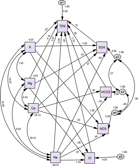
SEM of regression model 1
Table 6 Fit indices for SEM -
SEM 2
This model is obtained from SEM 1 by excluding the direct relationship between TDS and K+. Figure 4 shows SEM 2, and as in the case of SEM 1, the regression coefficients for TDS are almost the same to those of the MLR model 2 in Table 4. Regarding the model fit, Table 6 shows that there is a slight improvement in the χ 2 value, while other fit indices are very close. AGFI again shows an acceptable fit and not a good fit. From Table 6 and Fig. 4, it can be concluded that the SEM study agrees with the MLR method.
Fig. 4 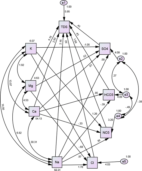
SEM of regression model 2 (with K+→TDS relation excluded)
-
SEM 3
Similar to SEM 2, this model is obtained from SEM 1 by excluding the direct relationship between TDS, K+, HCO3 − and SO4 2−, exactly as in the case of MLR model 3. Figure 5 shows SEM 3. An examination of Fig. 5 and Table 5 reveals the same regression coefficients for predicting TDS, in the case of SEM 3 and MLR model 3. However, according to Table 6, the fit indices are not satisfactory, especially the AGFI which does not even indicate an acceptable fit. This again justifies our earlier decision to accept MLR model 2 in predicting TDS based on the data analyzed.
Fig. 5 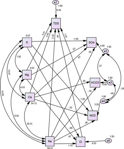
SEM of regression model 3 (with K+, HCO3 −, SO4 2−→TDS relations excluded)


Table 6 shows that for all the three SEMs, the fit index TLI is very close to 1, which indicates a very good fit. Since TLI is relatively independent of the sample size, we can accept the models developed even though our sample size is small.
4 Conclusion
A multivariate statistical study of the physico-chemical parameters of the ground water of the Kozhikode District, Kerala State, India was conducted. First a linear regression model involving TDS and EC was developed, which revealed a comparatively lower TDS/EC ratio. A PCA was then carried out for identifying a possibly lesser number of variables which contain the essence of the entire data. Hence, a regression model for predicting TDS using the parameters HCO3 −, SO4 2−, NO3 −, Cl−, Ca2+, Mg2+, K+ and Na+ was formed. This model was then modified by excluding the less significant parameter K+. A third regression model was then developed by excluding less significant HCO3 − and SO4 2−, where all the parameters were found significant. Due to lower values for R-square and MSE, the second model was selected for predicting TDS. Finally, the validity of the three regression models studied was tested using SEM, which revealed almost the same regression model for predicting TDS. Several fit indices indicated a very good SEM fit of the data besides the comparatively small sample size.
References
Ali MH (2010) Fundamentals of Irrigation and On-farm Water Management: Volume 1. Springer
Amiri BJ, Nakane K (2009) Modeling the linkage between river water quality and landscape metrics in the Chugoku district of Japan. Water Resour Manag 23:931–956
APHA (2012) Standard methods for the examination of water and wastewater. In: Eaton AD, Clesceri LS, Rice EW, Greenberg AE (eds) American Public Health Association, American Water Works Association and Water Environment Federation, 22nd edn. American Public Health Association, Washington DC
Ashley RP, Lloyd JW (1978) An example of the uses of factor analysis and cluster analysis in ground water chemistry interpretation. J Hydrol 39:355–364
Barrett P (2007) Structural equation modeling: adjudging model fit. Personal Individ Differ 42(5):815–824
Bentler PM (1988) Causal modeling via structural equation systems. In: Nesselroade JR, Cattell RB (eds) Handbook of Multivariate Experimental Psychology. Springer US, pp 317–335
Bentler PM (1990) Comparative fit indexes in structural models. Psychol Bull 107(2):238–246
Bhardwaj V, Singh DS, Singh AK (2010) Water quality of the Chhoti Gandak River using principal component analysis, Ganga Plain, India. J Earth Syst Sci 119(1):117–127
Bollen KA (1990) Overall fit in covariance structure models: two types of sample size effects. Psychol Bull 107(2):256–259
Byrne BM (2009) Structural Equation Modeling with AMOS. 2nd edition, Routledge
Chaudhary R, Rachana Pillai S (2009) Algal biodiversity and related physico-chemical parameters in Sasthamcottah Lake, Kerala (India). J Environ Res Dev 3(3):790–795
Chenini I, Khemiri S (2009) Evaluation of ground water quality using multiple linear regression and structural equation modeling. Int J Environ Sci Tech 6(3):509–519
Divya KR, Manonmani K (2013) Assessment of water quality of River Kalpathypuzha, Palakkad District, Kerala. IOSR J Environ Sci Toxicol Food Technol 4(4):59–62
Dunteman GH (1989) Principal Components Analysis. SAGE Publications, Inc
Eslamian S, Ghasemizadeh M, Biabanaki M, Talebizadeh M (2010) A principal component regression method for estimating low flow index. Water Resour Manag 24:2553–2566
Hem J D (1985) Study and Interpretation of the Chemical Characteristics of Natural Water. U.S. Geological Survey, Water Supply Paper 2254. http://pubs.water.usgs.gov/wsp2254
Hincks SS, Mackie G (1997) Effects of pH, Calcium, alkalinity, hardness and chlorophyll on the survival, growth and reproductive success of zebra mussel (Dreissena polymorpha) in Ontario lakes. Can J Fish Aquat Sci 54:2049–2057
Hoelter JW (1983) The analysis of covariance structures: goodness-of-fit indices. Sociol Methods Res 11:325–344
Hooper D, Coughlan J, Mullen MR (2008) Structural equation modeling: guidelines for determining model fit. Electron J Bus Res Methods 6(1):53–60
Iacobucci D (2010) Structural equations modeling: fit indices, sample size, and advanced topics. J Consum Psychol 20:90–98
Joji VS (2009) Ground water information booklet of Kozhikode district, Kerala state. Central Ground Water Board, Min. of Water Resources, Govt. of India. www.cgwb.gov.in/District_Profile/Kerala/Kozhikode.pdf
Joseph PV, Claramma J (2010) Physicochemical characteristics of Pennar River, a fresh water wetland in Kerala, India. E- J Chem 7(4):1266–1273
Kerala Vision 2030 (2014) http://www.kerala.gov.in/docs/reports/vision2030
Kim J, Mueller CW (1978) Introduction to factor analysis: what it is and how to do it. SAGE Publications
Kline RB (2005) Principal and practice of structural equation modeling, 3rd edition. The Guilford Press
Koklu R, Sengorur B, Topal B (2010) Water quality assessment using multivariate statistical methods-A case study: Melen River system (Turkey). Water Resour Manag 24:959–978
Kotti ME, Vlessidis AG, Thanasoulias NC, Evmiridis NP (2005) Assessment of river water quality in Northwestern Greece. Water Resour Manag 19:77–94
Kozhikode (2014) In Wikipedia, The Free Encyclopedia. Retrieved 07:31, September 2, 2014, from http://en.wikipedia.org/w/index.php?title=Kozhikode&oldid=623449938
Laxmilatha P, Thomas S, Asokan PK, Surendranathan VG, Sivadasan MP, Ramachandran NP (2009) Mussel farming initiatives in north Kerala, India: a case of successful adoption of technology, leading to rural livelihood transformation. Aquacult Asia 14(4):9–13
Locsey KL, Cox ME (2003) Statistical and hydrochemical methods to compare basalt- and basement rock- hosted ground waters: Atherton Tablelands, north-eastern Australia. Environ Geol 43(6):698–713
Marsh HW, Balla JR, McDonald RP (1988) Goodness-of-fit indexes in confirmatory factor analysis: the effect of sample size. Psychol Bull 103(3):391–410
Mazlum N, Ozer A, Mazlum S (1999) Interpretation of water quality data by principal components analysis. Tr J Eng Environ Sci 23:19–26
Olsen RL, Chappell RW, Loftis JC (2012) Water quality sample collection, data treatment and results presentation for principal components analysis-literature review and Illinois River Watershed case study. Water Res 46(9):3110–3122
Petersen W, Bertino L, Callies U, Zorita E (2001) Process identification by principal component analysis of river water-quality data. Ecol Model 138:193–213
Prescott K, Claudi R (2012) Examination of water quality in clear lake, California for Dreissenid Mussel suitability. Report for California Department of Water Resources, Aquatic Nuisance Species Program. http://www.rntconsulting.net/Publications/Articles.aspx
Reeder SW, Hitchon B, Levinson AA (1972) Hydrogeochemistry of the surface waters of the Mackenzie River drainage basin, Canada-I. Factors controlling inorganic composition. Geochim Cosmochim Acta 36(8):825–865
Schermelleh-Engel K, Moosbrugger, Muller H (2003) Evaluating the fit of structural equation models: tests of significance and descriptive goodness - of - fit measures. Methods Psychol Res 8(2):23–74
Shaji C, Nimi H, Bindu L (2009) Water quality assessment of open wells in and around Chavara industrial area, Quilon, Kerala. J Environ Biol 30(5):701–704
Shlens J (2003) A Tutorial on principal component analysis. arXiv:1404.1100 [cs.LG]
Subin MP, Miji PM (2013) Impact of certain pollution sources on microbiology and physicochemical properties of bore well water in the northern part of Ernakulam District in Kerala. India Int Res J Environ Sci 2(1):1–8
Sujitha PC, Mitra DD, Sowmya PK, Priya RM (2012) Physico-chemical parameters of Karamana River water in Trivandrum District, Kerala, India. Int J Environ Sci 2(3):1417–1434
Suk H, Lee KK (1999) Characterization of a ground water hydrochemical system through multivariate analysis: Clustering in to ground water zones. Groundwater 37(3):358–366
Warne RT, Larsen R (2014) Evaluating a proposed modification of the Guttman rule for determining the number of factors in an exploratory factor analysis. Psychol Test Assess Model 56(1):104–123
Westland JC (2010) Lower bounds on sample size in structural equation modeling. Electron Commerce Res Appl 9(6):476–487
Wolf EJ, Harrington KM, Clark SL, Miller MW (2013) Sample size requirements for structural equation models an evaluation of power, bias and solution propriety. Educ Psychol Meas 73(6):913–934
Wood WW (1976) Guidelines for collection and field analysis of ground-water samples for selected unstable constituents. USGS Techniques of Water-Resource Investigation : 01-D2
Wurts WA (1993) Understanding water hardness. World Aquacult 24(1):18
Acknowledgments
The authors gratefully acknowledge support from the: Centre for Water Resources Development and Management (CWRDM) Kozhikode; Kerala Water Authority (KWA) Kozhikode; Department of Chemical Engineering and Department of Chemistry, Govt. Engg. College, Kozhikode towards testing the physic-chemical parameters of the water samples collected; Department of Town and Country Planning, Kozhikode for providing maps of Kozhikode district. We also acknowledge the editor and the anonymous reviewers for their valuable suggestions towards improving the standards of the paper.
Author information
Authors and Affiliations
Corresponding author
Rights and permissions
About this article

Cite this article
Viswanath, N.C., Kumar, P.G.D., Ammad, K.K. et al. Ground Water Quality and Multivariate Statistical Methods. Environ. Process. 2, 347–360 (2015). https://doi.org/10.1007/s40710-015-0071-9
Received:
Accepted:
Published:
Issue Date:
DOI: https://doi.org/10.1007/s40710-015-0071-9