
Abstract
With the global consciousness of climate change, renewable energy systems are prioritized over the conventional energy systems. The deep injection of renewables into the power systems is creating several challenges to the grid due to wide variations in their output power depending on the time of the day, weather etc. Of these challenges, frequency change plays a vital role in maintaining the power quality. This paper presents a novel sliding mode controller with non-linear disturbance observer to effectively mitigate the wide changes in the frequency. A sliding mode surface based on estimated disturbance along with states is designed. A sliding mode control law is proposed to compensate disturbances including variations in renewables, load and parameters under mismatched uncertainties. The proposed observer based controller is tested for three area multi-machine power system in MATLAB/Simulink. The simulated results proved to alleviate the frequency variations effectively compared to the conventional controllers.
1 Introduction
Renewable energy systems have become the cog in the wheel of power systems due to the outcry on global warming. Also, most of the emerging countries are trying to shift towards green energy systems by changing their policies towards carbon negativity. Among those renewables, wind and solar plants are mushrooming due to their availability. But the major disadvantage of the wind and solar energy is their stochastic nature as they depend on the weather conditions. This poses a serious threat to power system stability. Increased penetration of wind energy leads to increased rate of variation of net load demand on the grid with reduced operational stability [1]. Large scale integration of wind energy may lead to increase in inter-area oscillations [2]. When these sources are synchronized with thermal power generation stations, there are many issues arising such as increased frequency fluctuations, increased losses and reduced operating efficiency.
Automatic generation control (AGC) is used to balance the power and counteract the frequency variations. Power system security and stability greatly depends on the effectiveness of AGCs in the thermal power plants to counteract the power imbalance [3]. There are several traditional methods that address the load frequency control such as integral, proportional-integral (PI) and proportional-integral-differential (PID) controllers. The performance of these controllers greatly depends on the controller parameter values [4]. The major issue with these controllers is disturbance attenuation or compensation. Other issues are conventional controllers cannot handle parameter variations, load variations and unmodelled dynamics. Frequency regulation by controlling load side demand is proposed in [5]. But this method is not viable for large power systems with multiple load centers and generating units. Takagi-Sugeno fuzzy model of power systems is considered for the design of fuzzy based frequency control in [6]. Large disturbances in wind & solar energy, load and parameter variations has drastic effect on the frequency. Thus there is a need to compensate these disturbances. The effect of disturbance can be minimized by estimating and compensating the disturbance. Disturbance affecting the system can be estimated using linear disturbance observer, extended state observer [7], nonlinear disturbance observer etc. For matched uncertainty, disturbances can be estimated and are compensated directly through control input [8]. When the case of mismatched uncertainties arise, the direct compensation through control input is not effective.
Sliding mode control is one of the robust control tools that can handle the various disturbances on the system. Because of the advantages like insensitivity to parameter variations, external disturbances, unmodelled dynamics and finite time convergence of sliding surface, the applications of sliding mode control are not limited to speed control of PMSM [9], sensorless speed control of induction motor [10], missile control [11] etc. A normal sliding mode control cannot effectively handle mismatched uncertainty. Sliding mode control is used for frequency control of thermal and hydro power plants [12]. The effect of parameter variations and the effect of renewables are not discussed. Sliding mode frequency control for multi-machine power systems with matched uncertainty and mismatched uncertainty was proposed in [13]. A disturbance observer based sliding mode control (DO-SMC) for frequency regulation is proposed in [14, 15]. But this method requires two functioning controllers. One controller is integral controller for handling steady state conditions and the other is sliding mode control for compensating disturbances. In this paper a novel sliding mode surface, as a function of states and estimated disturbance, is proposed for frequency control. The disturbance in the system is estimated using nonlinear disturbance observer. This proposed controller serves dual function of controlling the system under normal conditions as well as compensating the disturbance.
The paper is organized as follows. Section 2 discusses the configuration of hybrid energy system under study. Section 3 outlines the procedure for nonlinear disturbance observer design and the design of sliding mode controller. Disturbance observer and sliding mode controller are designed for the proposed system in Section 4. Section 5 analyzes the simulated results for the proposed system.
2 System configuration under study
The system under study is a three area multi-machine power system as shown in Fig. 1. Area-1 consists of thermal power generator synchronized with wind and solar power generators which are connected to load center as shown in Fig. 2. Area-2 and Area-3 consists of thermal power generators connected to load centers. The intermittent nature of renewable energy sources leads to large frequency fluctuations in Area-1. The conventional PI or PID controllers may not deal with this issue. The system performance can be improved by compensating the disturbance. Therefore the objective of this paper is to design a frequency controller for Area-1 that can stabilize the overall system even under multiple disturbances.

Hybrid energy system

Area-1 with renewable energy sources
The power system is a more complex and distributed system. It displays highly non-linear behavior due to constantly changing dynamics in the systems. This becomes more profound when parameter changes are also to be considered. In conjunction with the load-demand, the generation is also increasing rapidly. This paved a way for exhaustive integration of renewables into the system. This leads to large disturbances owing to the stochastic nature of the renewables. Conventionally, the operating point may be preserved by forecasting the renewable energy. But, the validity of the intraday forecast itself is questionable due to intermittent weather conditions.
Generally, the power system is linearized at an operating point and the controller is designed so that the system operates at that point. If the system deviates far from the operating point, severe non-linearities are introduced and the conventional controller may lose its control over the system.
In this paper, a linearized model of power system for ith area with thermal, wind and solar energy systems is considered.
where \(\Delta f_{i}\) is the change in frequency; \(\Delta P_{gi}\) is the change in generator power output; \(\Delta P_{di}\) is the change in load demand; \(\Delta P_{wi}\) is the change in wind power input; \(\Delta P_{si}\) is the change in solar power input; \(K_{Pi}\) is power system gain; \(T_{Pi}\) is the power system time constant; \(T_{Ti}\) is the turbine time constant; \(\Delta X_{gi}\) is the change in governor valve position; \(T_{Gi}\) is the governor time constant; \(R_{i}\) is the speed regulation coefficient; \(u_{i}\) is the control input; \(\Delta \delta_{i}\) is the rotor angle deviation; \(K_{sij}\) is the interconnection gain; \(\psi\) denotes unmodelled dynamics and change in parameter values.
All the load variations, unmodelled dynamics, parameter variations and renewable energy changes are treated as lumped disturbance on the system.
Accordingly (1) is modified as:
where \(d_{i}\) denotes the lumped disturbance on the system, is expressed as:
3 Disturbance observer based sliding mode control
Let us consider a dynamic system in the form of
where \(\varvec{x} \in {\mathbf{R}}^{n}\) is the state vector; \(\varvec{u} \in {\mathbf{R}}^{m}\) is the control vector; \(d\left( {\varvec{x},t,w} \right)\) is the net disturbance on the system; \(\varvec{y}\) is output vector; \( \varvec{B}_{1} = \left[ {\begin{array}{*{20}l} 0 \hfill & b \\ \end{array} } \right]^{\text{T}} \); \( \varvec{B}_{2} = \left[ {\begin{array}{*{20}l} 1 \hfill & 0 \\ \end{array} } \right]^{\text{T}} \); \( \varvec{C} = \left[ {\begin{array}{*{20}l} 1 \hfill & 0 \\ \end{array} } \right]^{\text{T}} \); \( \varvec{A} = \left[ {\begin{array}{*{20}l} 0 \hfill & 1 \\ {a_{1} } \hfill & {a_{2} } \\ \end{array} } \right] \).
Assumption 1
This system comes under the case of mismatched certainty. This is because \(\varvec{B}_{1} \ne \lambda \varvec{B}_{2}\), where \(\lambda\) is a scalar.
Assumption 2
The net disturbance on the system is assumed to be bounded i.e. \(d < d_{m}\), where d m is a scalar.
3.1 Control structure
The proposed control structure is shown in Fig. 3. It consists of a disturbance observer that estimates the lumped disturbance on the system based on the states and the control law. The estimated disturbance is given to the sliding-mode controller which compensates the disturbance and controls the states.

Disturbance observer
3.2 Disturbance observer design
Initially, a disturbance observer is designed to compensate the disturbances in the system. The structure of disturbance observer is shown in Fig. 4.
where \(\hat{d}\) is the estimated disturbance; \(\beta\) is the virtual state; \(\varvec{G}\) is disturbance observer gain to be designed.

Sliding mode control
Taking the derivative of (9)
If \(\varvec{GB}_{2} > 0\), then
3.3 Design of sliding mode controller
The design of sliding mode controller involves two steps. The first being the design of sliding surface and the second is the design of control input as shown in Fig. 5. A novel sliding surface based on the states and disturbance estimation is formulated as:
where k > 0 is the parameter to be designed.

Sliding mode controller
Sliding mode control input is designed as:
Differentiating (12) leads to
4 Controller design for proposed system
The above mentioned concept of control can be used for design of decentralized frequency regulator in multi-machine power systems. The system (see (2)–(4)) is represented in dynamic state space form as:
where \(\varvec{x} = \left[ {\begin{array}{*{20}l} {\Delta f_{i} } \hfill & {\Delta P_{gi} } \hfill & {\Delta X_{gi} } \hfill \\ \end{array} } \right]^{\text{T}}\)
The parameters of the system under study are given in Appendix A. As discussed earlier, the controller is designed for Area-1 where cumulative disturbance is maximum. The matrices for Area-1 are given below.
Transforming the system represented in (15) using the transformation matrix T c such that the new state vector \(\varvec{\xi}= \varvec{T}_{c} \varvec{x}\), where \(\varvec{T}_{c} = \left[ {\begin{array}{*{20}l} \varvec{C} \hfill & {\varvec{CA}} \hfill & {\varvec{CA}^{2} } \end{array} } \right]^{\text{T}}\), \(\varvec{\xi}= \left[ {\begin{array}{*{20}c} {\xi_{1} } \hfill & {\xi_{2} } \hfill & {\xi_{3} } \end{array} } \right]^{\text{T}}\).
The new modified system obtained is given below.
The above system is represented as:
where \(\varvec{A}_{C} = \varvec{T}_{c} \varvec{AT}_{c}^{ - 1}\); \(\varvec{B}_{C} = \varvec{T}_{c} \varvec{B}_{1}\); \(\varvec{D}_{C} = \varvec{T}_{c} \varvec{B}_{2}\).
There exists
The objective of this paper is to design control input that stabilizes the system operating frequency by counteracting the disturbances.
The lumped disturbance of the system is estimated using nonlinear disturbance observer as given in [16]. The dynamics of the disturbance observer for estimating the disturbance on the system are given below.
The matrix G is to be designed such that the eigenvalues of GB C lie on the left half of s-plane.
To address the uncertainties including variations in wind and solar energy generation, the disturbance observer based sliding surface is formulated as:
where k1, k2, k3 are constants to be selected such that the roots of (23) lie on the left half of s-plane.
A control input is designed to stabilize the system operating frequency.
-
1)
Stability proof
Let us consider the Lyapunov function as:
$$V = \frac{1}{2}\rho^{2}$$(25)Taking the derivative of (25), there exists
$$\begin{aligned} \dot{V} & = \rho \dot{\rho } = - \gamma \left| \rho \right| + \\ & \quad \left( {k_{1} - 0.05k_{2} + 0.002k_{3} + \varvec{GD}_{C} } \right)\left( {\hat{d} - d} \right)\rho \le \\ & \quad - \left[ {\gamma - \left( {k_{1} - 0.05k_{2} + 0.002k_{3} + \varvec{GD}_{C} } \right)\left( {d_{m} - \hat{d}} \right)} \right]\left| \rho \right| \\ \end{aligned}$$(26)If \(\gamma > \left( {k_{1} - 0.05k_{2} + 0.002k_{3} + \varvec{GD}_{C} } \right)\left( {d_{m} - \hat{d}} \right)\), then the stability of the sliding mode control can be guaranteed.
-
2)
Remarks
-
a)
In the absence of disturbances and parameter variations, the function of proposed sliding mode control is similar to conventional sliding mode control.
-
b)
Even for large variation in actual and estimated disturbance, from (10) and (11), the estimated disturbance tracks the true value in finite time.
-
c)
It can handle both steady state and transient conditions.
-
a)
5 Simulation results
The proposed controller is tested on a three-area multi-machine power system discussed in Section 2 in a simulated environment using MATLAB/Simulink ver.2009a with Ode4 solver and a sample time of 1 ms. The proposed controller is applied for Area-1 and PI controllers are used in the other two areas.
The following values are selected for the design of the controller and non-linear disturbance observer: \(\varvec{G} = \left[ {\begin{array}{*{20}l} {10} \hfill & 0 \hfill & {0.01} \end{array} } \right]\), \(k_{1} = 575\), \(k_{2} = 48\), \(k_{3} = 1\), \(\gamma = 100\).
-
1)
Case 1: effect of load disturbance
In this case, only load disturbance is considered without wind and solar power input to the system. Load is suddenly increased by 0.1 p.u. With nonlinear disturbance observer, the net disturbance is estimated and the true value of disturbance is tracked within a short period though initial condition of the observer is different from the actual and the same is shown in Fig. 6. From the figure it can be observed that the disturbance observer is able to track the actual disturbance in 0.4 s. Due to the variation in estimated and actual disturbance along with the states, the sliding surface is also seen to be non-zero. The sliding surface ρ reaches zero when the states and disturbance tracks the true value as shown in Fig. 7. The control input to the system is shown in Fig. 8. In Fig. 9, the effectiveness of regulating the frequency with sliding mode control is compared with conventional PI controller. It can be observed that with PI controller, the change in frequency has an undershoot of − 0.25 Hz. But with DO-SMC, the undershoot of change in frequency reduced significantly to − 0.065 Hz. Also the settling time in the proposed control is very small compared to the conventional PI controller.
Fig. 6 
Actual and estimated disturbance
Fig. 7 
Sliding surface for load disturbance
Fig. 8 
Control input
Fig. 9 
Change in frequency
From this we can infer that the performance of DO-SMC is superior in terms of peak overshoot, settling time and disturbance rejection.
-
2)
Case 2: effect of generation rate constraint (GRC)
To represent practical power systems, GRC is included in the simulation model [17, 18]. Figure 10 shows the change in frequency for a 5% step load change with a GRC value of 0.005 p.u.MW/s. However, due to GRC, the settling time is increased.
Fig. 10 
Change in frequency with GRC
-
3)
Case 3: effect of governor dead band and time delay
Further, the performance of the proposed controller is evaluated by inserting other nonlinearities like governor dead-band and actuator time delay along with GRC in the model [17, 18]. The change in frequency with GRC of 0.005 p.u.MW/s, governor dead band (GDB) as 5% and delay time as 0.05 s is shown in Fig. 11. The proposed controller is robust to above said non-linearities.
Fig. 11 
Change in frequency with GRC, GDB and time delay
-
4)
Case 4: effect of wind variations
In this case, wind generation is modeled as a Gaussian noise with 0.1 p.u. mean and variance of 10−4 to represent the physical system. The wind input is shown in Fig. 12. The continuous variation in wind generation leads to large fluctuations in operating frequency with conventional controller. The applied nonlinear disturbance observer tracks even fast changing disturbances and is shown in Fig. 13. Since the sliding surface ρ is a function of disturbance as well as states, it changes continuously with the disturbance as shown in Fig. 14. Frequency distortions are drastically reduced with sliding mode controller when compared to PI controller as shown in Fig. 15. The corresponding control input with variable wind generation is shown in Fig. 16.
Fig. 12 
Wind input
Fig. 13 
Actual and estimated disturbance for wind variations
Fig. 14 
Sliding surface for wind variations
Fig. 15 
Change in frequency for wind variations
Fig. 16 
Control input for wind variations
-
5)
Case 5: effect of multiple disturbances
In this case, the system is inflicted with wind, solar and load disturbances leading to more severity. Similar to wind, solar generation is also modeled as a Gaussian noise with mean of 0.01 p.u. and variance of 10−6. This solar model injects low amplitude, high frequency disturbances into the system. Along with this the load is suddenly reduced by 5% which will add to the disturbance created by the renewable generation. The disturbance observer based estimated lumped disturbance is shown in Fig. 17. Sliding surface, control input and change in frequency are shown in Figs. 18, 19 and 20 respectively. The frequency deviation with sliding mode control is slightly high initially because of the deviation of estimated disturbance. When disturbance estimated tracks the true value, the frequency deviation is drastically reduced. This shows the superior performance of the proposed sliding mode controller.
Fig. 17 
Actual and estimated disturbance for multiple disturbances
Fig. 18 
Sliding surface for multiple disturbances
Fig. 19 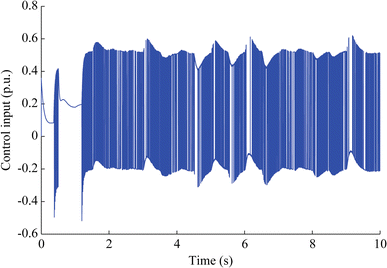
Control input for multiple disturbances
Fig. 20 
Change in frequency for multiple disturbances
-
6)
Case 6: effect of parameter variations
Most of the practical systems are subjected to parameter variations and this in turn affects the overall performance of the system. Thus there is a need to compensate the parameter variations. To examine the proposed controller for parameter variations, the system is simulated under time varying parameters.


A time varying parameter in the function of cos(t) are introduced in (4) and this is represented in (27).
The simulation results show that frequency changes with and without parameter variations are similar as shown in Fig. 21. Thus frequency change with parameter variation is negligible with the proposed sliding mode control.

Change in frequency with and without parameter variations
6 Conclusion
A non-linear observer is designed for estimating the lumped disturbance on the system. A control law for compensating the lumped disturbance based upon a novel sliding surface for frequency regulation in power system is proposed in this paper. The proposed system is tested on a three area multi-machine power system under various operating conditions. The sliding surface varies with the estimated disturbance facilitating limited variation in frequency. The results for all the cases, renewable disturbance, non-linearities (GRC, GDB and time delay), load perturbations and parameter variations, are shown to be superior compared to the conventional controllers. The proposed control law can be extended to large scale power systems with FACTS devices.
References
Yuan X (2013) Overview of problems in large-scale wind integrations. J Mod Power Syst Clean Energy 1(1):22–25
He P, Wen F, Ledwich G et al (2013) Small signal stability analysis of power systems with high penetration of wind power. J Mod Power Syst Clean Energy 1(3):241–248
He P, Wen F, Ledwich G et al (2013) Effects of various power system stabilizers on improving power system dynamic performance. Int J Electr Power Energy Syst 46(1):175–183
Gozde H, Taplamacioglu MC (2011) Automatic generation control application with craziness based particle swarm optimization in a thermal power system. Int J Electr Power Energy Syst 33(1):8–16
Molina-Garcia A, Bouffard F, Kirschen DS (2011) Decentralized demand-side contribution to primary frequency control. IEEE Trans Power Syst 26(1):411–419
Lee H, Park J, Joo Y (2006) Robust load-frequency control for uncertain nonlinear power systems: a fuzzy logic approach. Inf Sci 176(23):3520–3537
Li S, Yang J, Chen WH et al (2012) Generalized extended state observer based control for systems with mismatched uncertainties. IEEE Trans Ind Electron 59(12):4792–4802
Shtessel Y, Edwards C, Fridman L et al (2014) Sliding mode control and observation. Birkhäuser, New York
Zhang X, Sun L, Zhao K et al (2013) Nonlinear speed control for PMSM system using sliding-mode control and disturbance compensation techniques. IEEE Trans Power Electron 28(3):1358–1365
Gennaro SD, Dominguez JR, Meza MA (2014) Sensorless high order sliding mode control of induction motors with core loss. IEEE Trans Ind Electron 61(6):2678–2689
Zhou J, Yang J (2015) Smooth sliding mode control for missile interception with finite-time convergence. J Guid Control Dyn 38:1311–1318
Vrdoljak K, Perić N, Petrović I (2010) Sliding mode based load-frequency control in power systems. Electr Power Syst Res 80(5):514–527
Mi Y, Fu Y, Wang C et al (2013) Decentralized sliding mode load frequency control for multi-area power systems. IEEE Trans Power Syst 28(4):4301–4309
Mi Y, Fu Y, Li D et al (2016) The sliding mode load frequency control for hybrid power system based on disturbance observer. Int J Electr Power Energy Syst 74:446–452
Wang C, Mi Y, Fu Y et al (2016) Frequency control of an isolated micro-grid using double sliding mode controllers and disturbance observer. IEEE Trans Smart Grid. https://doi.org/10.1109/TSG.2016.2571439
Yang J, Li S, Yu X (2013) Sliding-mode control for systems with mismatched uncertainties via a disturbance observer. IEEE Trans Ind Electron 60(1):160–169
Jiang L, Yao W, Wu QH et al (2012) Delay-dependent stability for load frequency control with constant and time-varying delays. IEEE Trans Power Syst 27(2):932–941
Zhang CK, Jiang L, Wu QH et al (2013) Delay-dependent robust load frequency control for time delay power systems. IEEE Trans Power Syst 28(3):2192–2201
Author information
Authors and Affiliations
Corresponding author
Additional information
CrossCheck date: 2 November 2017
Rights and permissions
Open Access This article is distributed under the terms of the Creative Commons Attribution 4.0 International License (http://creativecommons.org/licenses/by/4.0/), which permits unrestricted use, distribution, and reproduction in any medium, provided you give appropriate credit to the original author(s) and the source, provide a link to the Creative Commons license, and indicate if changes were made.
About this article

Cite this article
TUMMALA, A.S., INAPAKURTHI, R. & RAMANARAO, P.V. Observer based sliding mode frequency control for multi-machine power systems with high renewable energy. J. Mod. Power Syst. Clean Energy 6, 473–481 (2018). https://doi.org/10.1007/s40565-017-0363-3
Received:
Accepted:
Published:
Issue Date:
DOI: https://doi.org/10.1007/s40565-017-0363-3