A multidimensional examination of performances of HSR (High-Speed Rail) systems

Abstract

This paper deals with a multidimensional examination of the infrastructural, technical/technological, operational, economic, social, and environmental performances of high-speed rail (HSR) systems, including their overview, analysis of some real-life cases, and limited (analytical) modeling. The infrastructural performances reflect design and geometrical characteristics of the HSR lines and stations. The technical/technological performances relate to the characteristics of rolling stock, i.e., high-speed trains, and supportive facilities and equipment, i.e., the power supply, signaling, and traffic control and management system(s). The operational performances include the capacity and productivity of HSR lines and rolling stock, and quality of services. The economic performances refer to the HSR systems’ costs, revenues, and their relationship. The social performances relate to the impacts of HSR systems on the society such as congestion, noise, and safety, and their externalities, and the effects in terms of contribution to the local and global/country social-economic development. Finally, the environmental performances of the HSR systems reflect their energy consumption and related emissions of green house gases, land use, and corresponding externalities.

1 Introduction

The high-speed rail (HSR) systems as the rather innovative systems within the railway transport mode, particularly as compared to its conventional (rail) passenger counterpart, have been developing worldwide (Europe, Far East-Asia, and United States of America (USA)). Despite the common name, different definitions of these systems have been used as follows:

• Japan The HSR system called ‘Shinkansen’ (i.e., ‘new trunk line’) is defined as the main line along almost its entire length (i.e., route) where trains can run at the speed of at least and above 200 km/h. The ‘Shinkansen’ system’s network has been built with the specific technical standards (i.e., dedicated tracks without the level crossings and the standardized and special loading gauge). This HSR system represents a part of the overall Japanese Shinkansen transportation system [1].

• Europe The definition of HSR system includes (a) infrastructure, (b) rolling stock, and (c) compatibility of the infrastructure and rolling stock [2].

  • Infrastructure Infrastructure of the trans-European HSR system is considered a part of the Trans-European rail transport system/network. It is specially built and/or upgraded for the high-speed (HS) travel. This may include connecting lines and junctions of the new lines upgraded for the HS, and the stations located on them, where the train speeds must take into account the local conditions. The HSR lines include those specially built for the speeds equal to or greater than 250 km/h (Category I), those specially upgraded for the speeds of the order of 200 km/h (Category II), and those upgraded with the particular features resulting from the topographical relief or the town-planning constraints (Category III). Therefore, the Category I lines are exclusively considered as the real HSR lines.

  • Rolling stock The HS trains are designed to guarantee safe and uninterrupted travel at the speed of at least 250 and 300 km/h under the appropriate circumstances on the Category I lines, about 200 km/h on the specially upgraded Category II lines, and at the highest possible speed on the other Category III lines.

  • Compatibility of the infrastructure and rolling stock The HS trains are designed to be fully compatible with the characteristics of infrastructure, and vice versa, which influences the performances in terms of safety, quality, and cost of services.

• China According to Order No. 34, 2013 from China’s Ministry of Railways, the HSR system refers to the newly built passenger-dedicated lines with (actual or reserved) speed equal and/or greater than 250 km/h. Its specific acronym is China railway high-speed (CRH). In addition, a number of new 200 km/h express passenger and 200 km/h mixed (passenger and freight) lines have been building as the components of the country’s entire HSR network [3].

• USA (United States of America) The HSR system is defined as that providing the frequent express services between the major population centers on the distances from 200 to 600 mile (mi) with a few intermediate stops, at the speeds of at least 150 mph (mi/h) on the completely grade-separated, dedicated rights-of way lines (1 mi = 1.609 km). It is also considered as the system providing regional, relatively frequent services operated at the speeds from 110 to 150 mph between the major and moderate population centers on the distances between 100 and 500 miles with some intermediate stops, grade separated with some dedicated and shared tracks using the positive train control technology [4, 5]. In both cases, the HSR system has been expected to relieve congestion at the highways and airports, in the latter case particularly by competing with the short- to medium-haul airline flights.

This paper deals with a multidimensional examination of the infrastructural, technical/technological, operational, economic, social, and environmental performances of the above-mentioned HSR systems by providing their overview, analysis, and limited (analytical) modeling. In addition to the introductory section, this paper consists of eight other sections. Section 2 introduces the concept of performances of the HSR system(s). Section 3 analyzes the systems’ infrastructural, Sect. 4 technical/technological, Sect. 5 operational, Sect. 6 economic, Sect. 7 social, and Sect. 8 environmental performances. The last section summarizes some conclusions.

2 A concept of performances of HSR systems

The performances of transport systems can be defined as their ability to fulfill the needs and expectations of particular actors/stakeholders involved, which are usually users/passengers, rail operators, and the third parties. For the HSR systems, these performances can generally be classified as infrastructural, technical/technological, operational, economic, social, and environmental [6].

• Infrastructural and technical/technological performances imply the system’s physical, constructive, technological, and technical characteristics of infrastructure, vehicles, i.e., HS trains, and supporting facilities and equipment, i.e., the power supply, signaling, and traffic control/management system(s);

• Operational performances reflect the system’s capabilities to serve the specified volumes of user/passenger demand under given conditions;

• Economic performances express the costs and revenues, the latter based on the charges (prices) to users/passengers, and their relationship(s); and

• Social and environmental performances reflect the scale of the system’s effects and impacts on the society and environment, the later usually expressed in the monetary terms as the external costs, i.e., externalities, if internalized by the related policies.

The above-mentioned performances of the HSR systems are frequently considered individually although being inherently dependent and influential on each other as shown in Fig. 1.

Fig. 1

A potential relationship of the performances of HSR systems [6]

As can be seen, according to the ‘top-down’ approach, the infrastructural performances directly influence the technical/technological performances, thus causing their mutual influence as well as the influence between them and all other performances. According to the ‘bottom-up’ approach, the social/policy performances can directly influence the infrastructural and technical/technological performances, thus creating the mutual influence of these and all other performances.

3 Infrastructural performances of HSR systems

The infrastructure of HSR systems consists of lines with the rail tracks connecting the stations/stops along them and the end stations/terminuses, both considered exclusively as the above-mentioned Category I of the HSR lines. The lines and stations constitute the HSR network spreading over a given region, country, and/or a continent. Table 1 provides an illustration of the progress so far in developing the HSR networks at particular continents.

Table 1 Development of the HSR networks at particular continents [14, 50]

As can be seen, the longest HSR network currently operating and being under construction is in Asia, mainly thanks to the fast developments in China, followed by that in Europe. The last are those in both Americas and Africa.

3.1 Lines

The lines as links connecting particular stations as the nodes of HSR network are mainly characterized by their three-dimensional layout and geometry of tracks. The most relevant parameters of geometry of tracks are the distance between their centers, gauge, the maximum axle load, gradient, the minimum horizontal and vertical radius of curvature, the maximum cant and the maximum cant gradient, and the length of transition curves corresponding to the minimum curve radius. For example, in Europe, except track gauge (1,435 mm), all other parameters are dependent on the maximum design speed. In addition, the HSR tracks can be broadly ballasted and ballast less [7, 8]. The former are present at the most already built HSR lines, while the latter have been considered particularly for the lines with long segments of tunnels and/or bridges such as those in Japan.¹ In addition, they have been expected to increase the capacity of HSR lines, operating speed, reduce the maintenance costs through reducing the frequency of maintenance operations, and consequently increase the level of safety.

3.2 Stations

The HSR stations mainly characterized by location and design enable facilitation of the HSR system with its users/passengers. The main aspect of location as the nodes of corresponding HSR network is their number along particular lines. Then, it is their micro-location in urban areas/cities and often at airports, which should enable safe, efficient, and effective accessibility by individual (car) and mass urban public transit systems (bus, tram, light rail, metro, and regional rail).² Furthermore, it is their functional design, which includes (i) the track and platform technical aspects (number, arrangement, dimension, safety, and electrical, signaling, and communication systems); (ii) the user/passenger service and comfort aspects (accessibility, inter-modal transfer, security, ticketing and travel information, station facilities, etc.); and (iii) the environmental aspects (choice of building/construction materials and protection of the local environment from noise) [11, 12].

In particular, an additional important aspect of design of the HSR stations is the arrangement of tracks and platforms for users/passengers. In general, two main concepts have been used: the side platforms facing the track(s) by one side and the island platforms facing the tracks by both sides, as shown in Fig. 2a, b, respectively [11].

Fig. 2

Simplified schemes of arrangements of the platforms and tracks at the HSR station. a Line station with the side platforms and two passing and two stopping tracks [11]. b Begin/end station/terminus with the inland platforms (Tokyo Shinkansen) [24]

The safety aspect of design of the HSR stations is important for users–passengers and accompanies standing on the platforms in cases when the non-stopping trains are passing by at relatively high speeds. These people could be affected (sucked toward a passing train if standing too close to the platform edge) by air streams generated by the HS trains. For example, some research indicated that the people standing on the platforms at the distance of 2 m from the HS train passing by at the speed of 240 km/h could be under a real risk [13].

3.3 Network

The above-mentioned lines and stations constitute the HSR infrastructure network, which spreads over a given country (http://www.johomaps.com/eu/europehighspeed). Table 2 shows some characteristics of the main grid (eight national backbone lines) of the HSR network in China.

Table 2 Some characteristics of the main grid of China rail high-speed (CRH) network [10, 15] (https://en.wikipedia.org/wiki/High-speed_rail_in_China/)

The specificity of this (Chinese) compared to the other HSR rail networks worldwide, particularly those in Europe, is the length of lines between the end stations/terminuses, which varies from 1,000 to 2,400 km. In Europe, these lengths are much shorter and vary, for example, from 280 km between Berlin and Hamburg (Germany) to 770 km between Paris and Marseille (France) [14]. However, the experience so far has shown that the average travel distances on some of these long Chinese lines have been about 560–620 km, which appears comparable to some of their (long) European counterparts [15].

4 Technical/technological performances of HSR systems

The technical/technological performances of HSR systems relate to their rolling stock, i.e., high-speed trains (HSTs) and supportive facilities and equipment, i.e., power supply, signaling, and traffic control/management system(s).

4.1 Rolling stock

The HSR rolling stock, i.e., trains, are characterized by an optimized aerodynamic shape; fixed composition and bi-directional set; self-propelling, concentrated, or distributed power; interior signaling system(s); several braking systems; power electronic equipment; control circuits; computer network; automatic diagnostic system; particularly high level of reliability, availability, maintainability, and safety (RAMS); maintenance by inspection in fixed time intervals and preventively; and compatibility with infrastructure (track and loading gauge, platforms, catenary, etc.) [1]. Table 3 provides the selected technical/technological specifications for different HS trains. As can be seen, the maximum design speed varies from 250 to 350 km/h. The locomotives are powered by the electric energy. These are the so-called multi-system locomotives interoperable for at least two different electric power supply systems. The traction power varies from 5,500 to 13,200 kW/train set. The length of a train set is predominantly about 200 m, and the corresponding weight is between 350 and 450 tons. Typical configuration of an HS train set is 1 power car + 8 trailers + 1 power car. The performance metrics vary across the considered set of HS trains from 12 to 23 kW/seat.

Table 3 Technical/technological characteristics of different HS trains [51] (http://en.wikipedia.org/wiki/ICE_3; http://en.wikipedia.org/wiki/Siemens_Velaro; http://www.trainweb.org/tgvpages/tgvindex.html; http://en.wikipedia.org/wiki/New_Pendolino)

In addition, Fig. 3 shows the relationship between the performance metrics and the seat capacity of the selected HS trains.

Fig. 3

Relationship between the performance metrics and the seat capacity of HS trains (Table 3)

As can be seen, the performance metrics expressed by the installed traction per seat (kW/seat) decreases more than proportionally with the increase of the number of seats, thus indicating economies of the train size in terms of the installed (and required) traction. This indicates that the HS trains with higher seating capacity do not need to have the proportionally stronger traction.

As well, Fig. 4 shows the relationship between the maximum designed and operating speed of the HS trains [16].

Fig. 4

Relationship between the maximum design and maximum operating speed of the selected HS trains (http://en.wikipedia.org/wiki/List_of_high-speed_trains)

As can be seen, the speeds ranging from 200 to 320 km/h coincide with each other for many HS trains. Nevertheless, generally, with the increase of the maximum design speed, the positive difference between this and the maximum operating speed tends to increase. This particularly happens for the speeds ranging between 270 and 380 km/h. Consequently, at particularly high maximum design speeds (above 300 km/h), it is likely to expect the lower maximum operating speeds for about 10 %–20 %, as shown in this case.

4.2 Supportive facilities and equipment

The main supportive facilities and equipment of the HSR system in the given context are power supply, signaling, and traffic control/management system.

4.2.1 Power supply system

The power supply system is an integrated system including the high-voltage electric power lines, substations, contact line, HS trains, and the remote command and control system ensuring efficient, reliable, and safe supply of electric power to the HSR lines and trains, and consequently operations. The electrified networks for the HSR lines generally use the alternate current (AC) or direct current (DC). As given in Table 3, the typical voltage and frequencies are 25 kV 50 Hz AC, 1.5 kV DC, and 15 kV 16.7 Hz AC. The latest has been installed in Germany and supplied from the dedicated high-voltage network called the ‘Railway Frequency.’ The above-mentioned general system components can further be divided into two main components: the HSR electrical infrastructure and the HS rolling stock traction equipment [17].

4.2.2 Signaling systems

The different HSR signaling systems have been applied in different countries. For example, each European country has its own HSR signaling systems: in France it is Transmission Vole Machine (TVM), in Germany LinienZugBeeinflussung (LZB), in Spain German’s LZB (for speeds up to 300 km/h) and Electrique Bureau CABine (EBICAB) (for speeds up to 220 km/h), and in Italy Blocco Automatico a Correnti Codificate (BACC) (for speeds up to 250 km/h). In addition, the European rail traffic management system (ERTMS—Level 1 and/or 2) has been introduced on the particular lines in different countries as an alternative and/or a complement to the existing national systems [17].

The type of signaling system influences the length of a block of the track, which can be occupied exclusively by a single HS train. The number of such successive empty blocks determining the (breaking) distance between any pair of HS trains moving in the same direction depends of their maximum operating cruising speed and the breaking/deceleration rate(s).

4.2.3 Traffic control/management system

In general, at the HSR rail lines/networks the rail traffic control/management systems is fully computer supported and can include the following main components: TOC—train operation controller; PC—power controller; STC—signal and telecommunication controller; CCC—crew and car utilization controller; PSC—passenger service controller; and TSMC—track and structure maintenance controller. These components are usually accommodated in the same room with the corresponding staff [18].

5 Operational performances of HSR systems

The main operational performances of HSR systems are demand, capacity, and quality of services, the latest as an outcome from the dynamic interaction between the former two. These performances can be considered for an individual line/route and/or for the entire network serving a given region, i.e., country.

5.1 Demand

The demand for HSR services consists of the self-generated demand and the demand attracted from other transport modes on the competitive routes such as individual car, conventional railways, and air passenger transport (APT).

In general, the self-generated demand for HSR services has been stimulated by expansion of the HSR network and increase of the welfare in terms of the national gross domestic product (GDP). Figure 5 shows the relationship between the served passenger demand and the length of HSR network in Europe and China.

Fig. 5

Relationship between the annual passenger demand and the length of HSR networks in Europe and China (period 1995–2014) [3, 50, 52]

In both regions, the served passenger demand has grown linearly with the increase of the length of HSR networks. In terms of absolute values, the served passenger demand in China has exceeded that in Europe during the relatively short period of time (7 years), which has indicated the very strong user/passenger preference to the new CRH speed system as shown in Fig. 6.

Fig. 6

Development of the satisfied passenger demand in the European HSR and Chinese CRH speed network (period 1990–2014) [50, 52]

In Europe, the served passenger demand has continuously been growing during the specified period of time. In China, since the start of implementing the CRH speed network, the corresponding passenger demand has been growing tremendously and very quickly exceeded that in Europe. In both cases, this has been possible primarily thanks to expanding the HSR network as shown in Fig. 6 and the other above-mentioned demand-stimulating factors. Figure 7 shows the relationship between GDP and the satisfied HSR passenger demand in Japan during the observed period [19].

Fig. 7

Relationship between the satisfied passenger demand by Japanese Tokaido Shinkansen HSR system and the national gross domestic product (GDP) (period 2001–2015) [19]

As can be seen, the served passenger demand has increased more than proportionally with rising of GDP, thus indicating that GDP has generally been, is, and will continue to be a strong generator of demand in the given context.

The attracted and satisfied HSR passenger demand from other transport modes on the competitive routes has resulted from their competition. Figure 8 shows the passenger market share of HSR compared to that of APT dependence on the line travel time.

Fig. 8

Relationship between the market shares of HSR and APT, and the line/route travel time [40, 53–55]

As can be seen, the relative market share of HSR (that of APT is complement to 100 %) has decreased linearly (Europe, Japan) and more than linearly (China) with the increase of the line/route travel time within the given range.

5.2 Capacity

The capacity of HSR systems can generally be calculated for their components of infrastructure—stations, lines/routes, and rolling stock. In general, for the infrastructure components, the ‘ultimate’ and ‘practical’ capacity can be considered. Both are dependent on the operational rules and procedures providing a safe separation of trains while operating along the lines and at the stations in the same and/or different directions. These rules specify the minimum time separation between occupying the same section of the line(s) and/or of the station(s), which mainly influences their corresponding capacities. In addition, the transport work and productivity can be considered as the measures integrating in some way the capacity of infrastructure components and that of operations of the rolling stock.

5.2.1 Infrastructure components

5.2.1.1 ‘Ultimate’ capacity

• Line The ‘ultimate’ capacity of a given HSR line/route is defined by the maximum number of trains, which can pass safely through the selected ‘reference location’ on the line where it is counted under given conditions, i.e., usually constant demand for service. This capacity can be estimated as follows [20, 21]:

  $$\mu_{l} (T) = \frac{T}{{t_{ij/\hbox{min} } }},$$

  (1a)

  where i, j are the leading and trailing trains in the sequence of two successive trains (ij) passing through the ‘reference location’ for their counting, respectively, which can be any location along the open line/route; t _ij/min the minimum time interval at which the successive trains (i) and (j) moving in the same direction pass through this ‘reference location’ (min); and T is the period of time for calculating the ultimate capacity of particular infrastructure component (h).

  This minimum time interval (t _ij/min) in Eq. 1a is mainly influenced by the HS train’s maximum operating speed, acceleration and deceleration/braking performances, length, the way of its control, and also the spacing and design of the stations/terminuses, gradients along the line/route, and type of traffic control (signaling) system. In general, this time can be estimated as follows [22]:

  $$t_{ij/\hbox{min} } = \frac{{V_{j} }}{{a_{j}^{ - } (V_{j} )}} + \frac{{S_{b/j} + L_{i} }}{{V_{j} }},$$

  (1b)

  where i, j are the leading and trailing HS trains, respectively, of the pair of successive trains (in); V _j is the maximum operating speed of the trailing train (j) (km/h); a ⁻(V _j ) is the average deceleration rate of the trailing train (j) at the maximal braking rate (m/s°); S _b/j is the “buffer” zone for the trailing train (j) (m); and L _i is the length of the leading train (i) (m).

  The maximum operating speeds of HS trains are usually about 250–350 km/h. The deceleration³ rate a ⁻ varies, i.e., it generally increases with the decrease of speed during the breaking phase of trip. The buffer zone (typically of the length of S _b/j  = 100 m) is the distance added to the braking distance of trailing HS train to allow a margin for its safe separation from the leading train (i) [22, 23]. The train length is typically L = 200 or 400 m. The latter is the length of Eurostar and 2-unit German-designed Velaro train operating in China (Table 3).

• Station along the line/route If the leading train (i) is to stop and the trailing train (j) is to pass through a station along the line, the ‘reference location’ for counting trains, i.e., calculating the capacity, can be the exit signal of the station. The ‘ultimate’ capacity of the station in this case can be estimated as follows [6, 20]:

  $$\mu_{s/l} (T) = \frac{T}{{t_{ij/s/\hbox{min} } }},$$

  (1c)

  where t _ij/s/min is the minimum time interval at which the successive trains (i) and (j) pass in the same direction through the station (min).

  The minimum time (t _ij/s/min) in Eq. 1c can be estimated as follows: the leading train (i) after being dispatched from the station should be at least at the minimum breaking distance of the trailing train (j) at the moment when this arrives at the exit signal of the station, which in this case will allow it to proceed. In such case, the time (t _{i j/min}) in Eq. 1b can generally be extended by the dwell time of the train (i) at the station as follows:

  $$t_{ij/s/\hbox{min} } = \tau_{i} + \left[ {\frac{{S_{b/j} + L_{i} }}{{2a_{j}^{ - } (V_{j} )}}} \right]^{1/2} + \frac{{V_{j} }}{{a_{j}^{ - } (V_{j} )}},$$

  (1d)

  where τ _i is the dwell time of the leading train (i) at the station (min).

  The other symbols are analogous to those in the previous equations.

  At most HSR systems, the dwell time is typically τ = 2–3 min at the stations located along the lines/routes and τ = 5 min for those located at airports, the latter mainly due to enabling users/passengers to handle their baggage. This time also includes the time for closing the doors, setting up the conflict-free exit path, and dispatching the leading train (i).

• End terminus/station The ‘ultimate’ capacity in this case can be estimated as follows [6, 20]:

  $$\mu_{{s/{\text{arr}}}} (T) = \frac{T}{{t_{{ij/\hbox{min} /{\text{arr}}}} }},$$

  (1e)

  where t _ij/min/arr is the minimum time interval at which the successive trains (i) and (j) arrive at the entry signal of the given end station/terminus (min) as the ‘reference location’ for their counting.

  The time (t _ij/min/arr) in Eq. 1e can be estimated as follows:

  $$t_{{ij/\hbox{min} /{\text{arr}}}} = \frac{{V_{j} }}{{a_{j}^{ - } (V_{j} )}} + \left[ {\frac{{S_{b/j} + L_{i} }}{{2a_{j}^{ - } (V_{j} )}}} \right]^{1/2} + \tau_{ij} + \tau_{b} ,$$

  (1f)

  where τ _ij is the time for changing the route of trains (i) and (j) arriving at the end station/terminus of the given line/route (typically 10 s); and τ _b is the time of blocking the entrance of the end station/terminus by other trains(s) (typically 25 s).

  The other symbols are analogous to those in the previous equations.

• Begin terminus/station The ‘ultimate’ capacity in this case can be estimated as follows [6, 20]:

  $$\mu_{{s/{\text{dep}}}} (T) = \frac{T}{{t_{{ij/\hbox{min} /{\text{dep}}}} }},$$

  (1g)

  where t _ij/min/dep is the minimum time interval at which the successive trains (i) and (j) pass the exit signal of the given station/terminus as the ‘reference location’ for their counting (min).

  The time (t _ij/min/dep) in Eq. (1g) can be estimated as follows:

  $$t_{{ij/\hbox{min} /{\text{dep}}}} = \hbox{max} \left\{ {\left[ {\frac{{S_{b/i} + L_{i} }}{{2a_{i}^{ + } (V_{i} )}}} \right]^{1/2} + \frac{{V_{i} }}{{a_{i}^{ + } (V_{i} )}};\tau_{j/r} + \tau_{j/gl} + \tau_{j/cf} + \tau_{j/d} } \right\},$$

  (1h)

  where τ _j/r is the time for setting the exit path for the trailing train (j) in a given departing sequence (ij) (usually 10 s); τ _j/gl is the time for setting the green light for trailing train (j) in a given departing sequence (ij) (usually 25 s); τ _j/cf is the time of blocking exit of the station/terminus for departing trailing train (j) by other incoming and outgoing trains (usually 60–75 s); and τ _j/d is the dispatching time of the trailing train (j) in a given departing sequence (ij) (usually 30 s).

  The other symbols are analogous to those in the previous equations.

  Equation 1h indicates that the minimum time between departures of the successive trains (i) and (j) from the begin station/terminus should be set up as the maximum of two time periods: the time the leading train (i) needs to reach the minimum breaking distance from the trailing train (j) and the time for setting up a safe departure path for this trailing train (j).

Figure 9 shows examples of the above-mentioned ‘ultimate’ capacities of the HSR line/route and begin/end station/terminus dependent on the train’s maximum operating speed calculated by Eq. 1.

Fig. 9

Relationships between the ultimate capacity of the HSR line/route, begin/end station/terminus, and the maximum train operating speed

As can be seen, the line/route capacity decreases with the increase of speed if the same average deceleration/acceleration rate is applied (a = 0.5 m/s² for the speeds of V = 250–350 km/h). However, if this rate increases with the increase of speed (a = 0.5 m/s² for the speed of V = 250 km/h, a = 0.3 m/s² for the speed of V = 270 km/h, a = 0.4 m/s² for the speed of V = 300 km/h, and a = 0.5 m/s² for the speeds of V = 320 and 350 km/h), the capacity generally tends to increase. In the latest case, the capacity again decreases due to applying the same deceleration/acceleration rate to the increasing speed. Similar happens with the arrival and departure capacities of begin/end station/terminus, respectively. In all cases, the train length is assumed to be L = 400 m and the buffer distance S _b  = 100 m [22]. Consequently, the line/route capacity can be estimated as the minimum of the above-mentioned four ‘ultimate’ capacities. In practice, the ‘ultimate’ capacity of the HSR lines/routes and stations is typically μ = 13–15 trains/h.⁴ In addition, the required number of tracks at the end/begin station/terminuses can be determined as the product of the above-mentioned ‘ultimate’ capacities and the HS train’s dwell time at the stations—stop time at the line and the turnaround time⁵ at the begin/end station(s).

5.2.1.2 ‘Practical’ capacity

The ‘practical’ capacity of a given HSR line/route is defined as the maximum number of HS trains, which can be accommodated during the specified period of time under conditions when each of them is imposed an average delay [25]. However, in this case, the mutual interferences between the HSR services of equal priority operating on the above-mentioned Category I lines causing their delays are prevented by the stability of timetable. This implies that the maximum permissible delay of leading train in the sequence of two trains is defined in a way not to cause an additional delay of the following train. As such, this delay indicates some kind of the system’s margin allowing delays of the HS trains anyway. The longer delays causing disruption of the timetable occur generally due to other causes.

5.2.2 Rolling stock

The capacity of HSR rolling stock reflects its size expressed by the number of trains of a given seating capacity required to operate under the conditions specified in the timetable. These conditions are usually characterized by the service frequency during the given period of time (h, day) and the train’s turnaround time along the given line/route. Consequently, the required number of rolling stocks/trains to carry out at the specified service frequency on a given line, m _rs [T; f(T)], can be estimated as follows [6, 26]:

$$m_{rs} [T;f(T)] = f(T)\tau ,$$

(2a)

where f(T) is the train service frequency on a given line during time (T) (trains/h; trains/day) and τ is the average turnaround time of a train along a given line (h).

The service frequency f(T) in Eq. 2a can be either considered to be equal to the line/route ‘ultimate’ capacity determined by Eq. 1 or set up to satisfy the expected demand as follows [26]:

$$f(T) = \hbox{min} \left[ {\mu_{l} (T);\mu_{s/l} (T);\mu_{s/arr} (T);\mu_{{s/{\text{dep}}}} (T);\frac{D(T)}{\rho (T)s}} \right],$$

(2b)

where D(T) is the expected user/passenger demand on a given HSR line during time (T)(pax); ρ(T) is the average load factor on a given line during time (T) (ρ(T) ≤ 1.0); and s is the seat capacity of a train operating on a given line (seats/train).

The other symbols are analogous to those in the previous equations.

The train’s turnaround time (τ) increases with the increase of the operating time along the line/route (the ratio between the length of line/route and the operating speed), the number and duration of intermediate stops, all in both directions, including those at the beginning and end station/terminus, and vice versa. The train’s seat capacity is usually constant per service frequency indicating the above-mentioned homogeneous HS train fleet on a given line/route. For example, if the given line/route operates at the service frequency of f(T) = 15 trains/h, and if the average turnaround time per train is τ _l  = 4 h, the required number of trains will be m _rs (T) = 15 × 4 = 60. In addition, if the average train’s seat capacity is s = 485 (TGV Atlantique, see Table 3), the total number of required seats will be m _s (T) = 29,100.

5.3 Transport work and productivity

The transport work and productivity of a given HSR line/route can be calculated for the supply and demand sides. On the supply side, it counts the total offered number of seats during a given period of time. On the demand side, it counts the total number of used seats under the same conditions.

Based on Eq. 2, the transport work on a given line for the supply (s-km) (seat-kilometers) and demand (p-km) sides, respectively, can be calculated as follows [26]:

$${\text{TWS}}(T) = f(T) \times s \times d \quad {\text{and}} \quad {\text{TWD}}(T) = f(T) \times s \times \rho (T) \times d.$$

(3a)

Similarly, the productivity of both supply and demand sides of a given line expressed as the volumes of seat-km/h and pax-km/h, respectively, can be calculated as follows:

$${\text{TPS}}(T) = f(T) \times s \times v \quad {\text{and}}\quad{\text{TPD}}(T) = f(T) \times s \times \rho (T) \times V,$$

(3b)

where d is the length of a given line (km) and V is the operating speed of HS trains on a given line (km/h).

The other symbols are analogous to those in the previous equations.

As can be seen, the transport work increases with the increase of the length of line, service frequency, seat capacity per frequency, and load factor. The productivity increases with the increase of the service frequency, seat capacity, load factor per frequency, and the average train operating speed, and vice versa. For example, for the HS trains, each with the seat capacity of s = 485 seats and the average load factor ρ = 0.80, operating on the line of length of d = 500 km at the operating speed of V = 300 km/h and the service frequency in the single direction of f(T) = 15 trains/h, the transport work on the line’s demand and supply sides during the period of 1 h will be TWS = 15 × 500 × 485 = 3,637,500 (seat-km) and TWD = 15 × 500 × 485 × 0.80 = 2,910,000 (pax-km), respectively. The corresponding productivity under the same conditions will be TPS = 15 × 485 × 300 = 2,182,500 (seat-km/h) and TPS = 15 × 485 × 0.80 × 300 = 1,746,000, respectively (pax-km/h).

5.4 Quality of service

The quality of service provided by HSR systems can be expressed by the attributes such as schedule delay, trip time in combination with the reliability and punctuality of services, the comfort on board HS trains, and accessibility of the HSR stations [27].

5.4.1 Schedule delay

The schedule delay is defined as the difference between the desired and the available time of boarding a chosen HSR service. Under an assumption that the users/passengers familiar with the timetable arrive uniformly during the time between any two successive HS trains’ departures on the same line/route/direction, this delay can be roughly estimated as follows [28, 29]:

$${\text{SD}}(T) = \frac{T}{4f(T)},$$

(4a)

where all symbols are analogous to those in the previous equations. For example, for the service frequency of f(T) = 1 train/h, the schedule delay will be SD(T) = 15 min; for the service frequency of f (T) = 15 trains/h, the schedule delay will be SD = 1 min (T = 1 h or 60 min).

5.4.2 Trip time, reliability, and punctuality

• Trip time by HSR systems is much shorter than that of their conventional counterparts at the same lines/routes. The potential time savings on a given route can be estimated as follows:

  $${{\Delta }} = d/(1/V_{{\text{CON}}} - 1/V_{{\text{HSR}}} ),$$

  (4b)

  where d is the length of a given line/route (km); V _CON is the operating speed of the conventional passenger train (km/h); and V _HSR is the operating speed of the HS train (km/h). Figure 10 shows an example for this in Italy.

  Fig. 10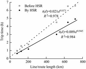

  

  Relationship between the trip time by the HS and conventional rail, and length of line/route in Italy [56]

  As can be seen, the difference in trip time by the conventional and HSR trains increases with the increase of the line/route length, which in the given case amounts to 33 %–42 %.

• Punctuality of the HSR services can be expressed by two attributes: (i) the ratio of the number of transport services carried out on time, i.e., according to the timetable, or with the specified maximum or average delays, and the total number of services carried out, and (ii) the average delay per delayed service. Both attributes are recorded during a given period of time (day, month, year) under given conditions. The experience so far has shown that these services in general and on the particular lines/routes have been highly punctual as shown in Fig. 11 [30].

  Fig. 11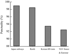

  

  Punctuality of services—the ratio—of the selected HSR systems [30]

  As can be seen, the Japanese HSR system has generally been the most and the UK’s the least punctual. In addition, Fig. 12 shows an example of the punctuality of the Japanese HSR system expressed by the average delay per service.

  Fig. 12

  

  Punctuality of services—the average delay—of the Japanese HRS system (period 1999–2008) [24, 57]

  As can be seen, the average delay per HSR service has varied from 0.3 to 0.5 min. In addition, the average delay of the Shinkansen HSR system has been about 0.6 min per service over the last decade [24, 31].

As can be seen, the average delay per HSR service has varied from 0.3 to 0.5 min. In addition, the average delay of the Shinkansen HSR system has been about 0.6 min per service over the last decade [24, 31].

• Reliability of the HSR services can be expressed as the ratio between the realized and planned transport services during a given period of time (day, month, and year) under given conditions. This is dependent on the rate of failure of rolling stock due to any system’s internal and/or external reasons causing cancelation or long delays of the affected services. Figure 13 shows an example of the Japanese HSR system.

  Fig. 13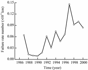

  

  Reliability of the HSR rolling stock (East Japan Railways—period 1987–2000) [24]

As can be seen, this rather very low failure rate has fluctuated during the observed period with an average of 0.084 failures/10⁶ km.⁶

5.4.3 Accessibility

Accessibility of stations is an important attribute of the overall quality of services provided by the HSR systems. In most cases, the new dedicated HSR stations are usually located and designed to fit as good as possible within the surrounding urban and/or sub-urban layout on one hand and enable the satisfactory quality of accessibility on the other. In some other cases, the parts of conventional railway stations have been appropriately upgraded and adapted to serve the HSR services. In both cases, the quality of accessibility needs is expected to be efficient, effective, and safe. This implies a reasonable (acceptable) time and costs from/to the doors of users/passengers by a variety of urban and sub-urban transit modes (car, taxi, and frequent, punctual, reliable, and safe, i.e., without incidents/accidents due to known reasons, bus, tram, metro, regional rail, etc.), respectively.

5.4.4 Comfort on board the HS trains

The comfort offered to their users/passengers on board of the HS trains usually includes the booked seats and the very limited number of stops along the lines/routes compared to those at the conventional train counterparts. As far as the comparison with the ATP system as the main competitor on the short- and medium-haul liens/routes is concerned, the attributes for comparison have usually been the distance between seats and internal mobility, diversity and type of services, noise on board, and the potential impact on health. Table 4 summarizes these for both systems/modes.

Table 4 Some attributes of the comfort on board of the HS trains and commercial passenger aircraft [30]

As can be seen, the HS trains have generally possessed higher comfort on board than their aircraft counterparts.

6 Economic performances of HSR systems

The economic performances of HSR systems include their costs and revenues. The costs are imposed by implementation and operation of the systems. The revenues obtained mainly by charging users/passengers cover the costs and provide some funds for updating the system and the profits for particular stakeholders involved. In any case, both revenues and costs need to be balanced in order to guarantee the economic and financial stability of the system.

6.1 Costs

The total costs of a given HSR system generally consist of the infrastructure and operating costs. The infrastructure costs include: (i) planning the system and acquisition and preparing the land; (ii) building the lines and stations including tunnels and bridges, and the supportive facilities and equipment including the signaling systems, catenaries and electrification mechanisms, and communications and safety installations; and (iii) maintenance of the entire infrastructure and supporting facilities and equipment [33]. The operating costs include acquiring, operating, and maintaining the rolling stock, selling services, and administration. The costs of labor, material, and energy have the largest share in the total costs [33].

Table 5 gives an indication of the average infrastructure cost of the already built and planned HSR lines, which do not include the cost of planning, and acquisition and preparation of the land.

Table 5 The average infrastructure cost of the HSR lines worldwide [3, 35, 42]

As can be seen, the average infrastructure cost for both already built and under-construction HSR lines has significantly varied in both European and non-European, i.e., two Asian countries. In Europe, the lowest cost has been in France and Spain, and much higher in Italy, Germany, and Belgium. It can be shown that the average infrastructure cost has been 18 million€/km. In addition, the average cost of building the new HSR lines in Asian countries (Japan, South Korea, except China) has been slightly higher than those in particular European countries [34, 35]. As well, the average maintenance cost per unit of length of the HSR system infrastructure has also highly varied, mainly depending on the length of lines. Some estimates indicate that the average maintenance cost in European countries has amounted from about 13–72 thousands/year [35, 36].

The average cost of operating the HSR services has also differed throughout the European counties and rest of the world as well. This cost has been mainly influenced by the local pricing of the particular above-mentioned inputs and type of the HS trains. Some estimates indicate that this average operating cost for 12 types of the HS trains operating in the corresponding European countries has been: $\overline{C} = 0. 1 4 6 2 6$ €/seat-km. In this total, the cost of maintenance of the rolling stock has shared about 8.5 %. Under an assumption that the average load factor was: θ = 0.8 (i.e., 80 %), the total average operating costs of the HSR services throughout Europe would be: $\overline{C} = 0. 1 8 3$ €/p-km [34, 35].

6.2 Revenues

The HSR systems obtain revenues from different sources such as the transport-based charging users/passengers, merchandise, and others [37]. In particular, the prices for users/passengers are set up to cover the systems’ total operating cost in cases of the lack of subsidies. The latter can be used as an element for enabling stronger competition with the other transport modes such as the conventional rail and particularly APT, both on the above-mentioned competitive lines/routes. Figure 14 shows relationship between the annual revenues and the annual satisfied demand of the HSR systems in different countries [19].

Fig. 14

Relationship between the annual revenues and the satisfied passenger demand of particular HSR systems—Japan, France, Germany, UK, USA (period 2012–2015) [19]

As can be seen, the revenues have generally linearly increased with increasing of the volumes of satisfied demand at an average of 17.44 ¢US$/p-km, which is in line with the above-mentioned corresponding costs.

6.3 Balancing revenues and costs

The HSR systems intend to operate in the profitable way, i.e., to cover their costs by revenues. Figure 15 shows an example of the profitability of the Japanese HSR operating both HSR and conventional rail services.

Fig. 15

Relationship between the annual demand and the net income/profits—Central Japan Company (period 2004–2013) [37]

As can be seen, despite a relatively high variations the profitability has generally increased with increasing of the volume of the company’s output during the given period of time. This case could be used as an example how the HSR system can be profitable in the medium- to long-term period—by careful balancing the revenues and costs while at the same time increasing the scale of operations to satisfy the growing user/passenger demand.

7 Social performances of HSR systems

The social performances of HSR systems include the impacts and effects. The impacts embrace noise, congestion, and safety, i.e., traffic incidents and accidents. The effects generally refer to the system’s overall welfare expressed by savings of the user/passenger time, relieving congestion from roads, and contribution to the regional GDP through direct and indirect employment.

7.1 Impacts

The HSR system generally impacts the society/people by noise, congestion, and safety, i.e., traffic incidents and accidents.

7.1.1 Noise

The HS trains generate noise while operating at the high speed(s), which comprises rolling, aerodynamic, equipment, and propulsion sound. This noise mainly depends on its level generated by the source, i.e., moving HS train(s), and its distance from an exposed observer(s). Figure 16 shows a scheme of changing the distance and time of exposure to noise by an HS train of an observer.

Fig. 16

Scheme for determining the noise exposure of an observer by passing by HS train [58]

The shadow polygon represents an HS train of length (L) passing by an observer (small triangle at the bottom) at the speed (V). He/she starts to consider noise of an approaching train when it is at distance (β) from the point along the line, which is at the closest right angle distance (γ) from him/her. The consideration stops after the train moves behind the above-mentioned closest point again for the distance (β). Under such circumstances, the distance between the observer and the passing-by HS train changes over time as follows:

$$\rho^{2} (t) = (L/2 + \beta - V \times \;t)^{2} + \gamma^{2} \quad {\text{for }}0 \, < t < = (L + 2 \times \beta )/V,$$

(5a)

where the last term represents duration of the noise event, i.e., the time needed for a train to pass by the observer (The length of HS trains is given in Table 3). If the level of noise received from the train passing by an observer with the speed (V) at the shortest distance (γ) is L _eq(γ, V), the level of noise at any time (t) can be estimated as follows:

$$L_{\text{e}} [\rho (t),V] = L_{\text{eq}} (\gamma ,V) - 8.6562\ln [\rho (t)/\gamma ].$$

(5b)

The second term in Eq. 5b represents the noise attenuation with distance over the area free of barriers. The total noise exposure of the observer from f(T) successive trains passing by during the period (T) can be estimated as follows:

$$L_{\text{eq}} [f(T)] = 10\log \sum\limits_{k = 1}^{f(T)} {10^{{\frac{{L_{e} [k,\rho (t),V]}}{10}}} } .$$

(5c)

As a standard approach, the noise from HS trains is measured at the right angle distance of $\gamma$ = 25 m from the track(s). Figure 17 shows the results of some such measurements across Europe depending on maximum operating speed of the HS trains.

Fig. 17

Relationship between the noise and the maximum operating speed of the passing-by HS train(s) measured at the right angle distance of 25 m (Belgium, France, Germany, Spain, Italy) [59]

As can be seen, the noise has generally linearly increased with increasing of the train’s operating speed: at the lower rate for the speeds up to about 300 km/h, and at the higher rate for the speeds above V = 300 km/h. The variation of noise level at the given speed has been about 3–4 dBA. This noise has included the train’s rolling (wheel), pantograph/overhead, and aerodynamic noise. Some additional measurements have shown that the rolling and pantograph/overhead noise has predominated and increased with increasing of the HS train’s speed approximately at the rate of 30lgV up to the speed(s) of about 300 km/h (some data have shown that this is 370 km/h). The aerodynamic noise depending on the HS train’s (aerodynamic) design has also increased, equalized with the rolling noise at the above-mentioned (transition) speed(s), started predominating and further increasing at an approximate rate of 80lgV [38]. In addition, in cases when the frequent HSR services are carried out along the particular lines/routes, their noise becomes persistent over time and can be estimated from Eq. 5c. As well, the time of exposure of an observer to noise by a passing by HS train can be estimated from Eq. 5a. If β = 0 m, L = 200 m, and v = 250 km/h, this exposure time to the maximum noise will be about t ₁ = 3 s; if V = 350 km/h, this time will be about t1 = 2 s.

Last but not least, while considering the actual exposure of the population located close to the HSR lines to noise by the passing-by HS trains, it is necessary to take into account the noise-mitigating barriers protecting the particular land use activities, i.e., a quiet land with intended outdoor use, a land with the residence buildings objects, and a land with the daytime activities (businesses, schools, libraries, etc.), all by absorbing the maximum noise levels for about 20 dB(A) (single barrier) and 25 dB(A) (double barrier).

7.1.2 Congestion

Thanks to applying the above-mentioned separation rules in addition to designing timetable(s) on particular lines/routes and the entire HSR network accordingly, the HSR systems are free of congestion and consequent delays due to the direct mutual influence of trains on each other while ‘competing’ to use the same segment of given lines/routes at the same time. However, the substantive delays due to some other reasons can propagate (if impossible to absorb and neutralize them) through the affected HS trains itineraries as well as along the dense lines/routes also affecting the other otherwise non-affected services. Under such conditions, the severely affected services are usually canceled in order to prevent further increase and propagation of their delays. On the one hand, this contributes to maintaining the punctuality but on the other, it compromises the reliability of the overall services (as mentioned above). Nevertheless, the already mentioned figures indicate that both reliability and punctuality of the HSR system services worldwide have been very and in some cases extremely high (The latter is the example of Japanese HSR system).

7.1.3 Safety, i.e., traffic incidents/accidents

Experience so far has indicated that the HSR and APT system have been the safest transport systems/modes in which traffic incidents/accidents have rarely occurred, usually due to the previously unknown reasons. This means that the number of traffic incidents/accidents and related person injuries, deaths, and the scale and cost of damaged properties both of the systems and the third parties per, for example, 10⁹ s-km and/or p-km carried out over a given period of time, have been extremely low. In particular, high safety of the HSR systems has been provided also a prior by designing completely the grade-separated lines and the other supportive built-in safety features at both infrastructure and rolling stock. This implies that the safety has been achieved on the account of increased investments and maintenance cost. As well, the HSR operators and infrastructure managers have continuously practiced a risk management and training approach aiming at maintaining a high level of safety and particularly with increasing of the maximum speeds. Nevertheless, the HSR systems in different countries have not been completely free from traffic incidents/accidents. For example, some relevant statistics for the TGV system in France indicate that there have not been accidents with the fatalities (deaths) and severe injuries of the users/passengers, staff, and/or third parties since starting the HSR services started in the year 1981 despite the trains have been carrying out annually about 10 × 10⁶ p-km. In addition, some incidents happened on the HSR lines/routes such as broken windows, opening of the passenger doors during operating at the cruising speed, couple of fires on board, collision with animals and concrete block on the tracks, and the terrorist attempts to bomb the tracks. The incidents and accidents of TGV trains operated on the conventional tracks have been more frequent with fatalities, injuries, and damages of properties but all at the relatively low scale. In these cases, the HS trains have been exposed to the external risk similarly to their conventional counterparts (http://www.railfaneurope.net/tgv/wrecks.html). Similarly, since started in 1960s, the Japan’s Tokaido Shinkansen HS services⁷ have also been free of accidents causing the user/passenger and staff fatalities and injuries due to the derailments and collisions of trains. This has been achieved despite the services have been exposed to the permanent threat of the relatively frequent (and sometimes strong) earthquakes.

Nevertheless, the fatal accidents with deaths and injuries of the users/passengers and staff happened at the HSR systems in Germany, Spain, and China (one in each country). Table 6 gives the main characteristics of these three accidents.

Table 6 Characteristics of the HSR fatal accidents [60–62]

7.1.4 Cost of the social impacts—externalities

Quantifying the social impacts of HSR systems in the monetary terms as externalities has usually represented an ambiguous and often politically challenging task. Nevertheless, some estimates of these externalities for the HSR systems and other transport modes in Europe have been carried out. They have indicated that the total social externalities of HSR systems have amounted 22.9 €/10³ p-km. In this total, the noise and traffic incidents/accidents externalities have shared about 22 % and 2 %, respectively. Since the HSR systems are free of congestion, the corresponding externality has not been considered. On the other hand, for comparison, the total externalities of APT have estimated to be 52.5€/10³ p-km, of which the noise and traffic incidents/accidents externalities shared about 4 % and 3 %, respectively [39, 40].

7.2 Effects

The effects of HSR systems have consisted of contribution to the direct and indirect employment and consequently the economic-social development and welfare, both at a global-country and the local–regional scale.

7.2.1 Direct employment

The direct employment relates to manufacturing, building, and maintaining the infrastructure and manufacturing, operating, and maintaining the rolling stock and supporting facilities and equipment, i.e., the main system’s components, of the HSR systems. For example, the number of employees operating the HSR services in particular countries is strongly dependent on the length of HSR networks as shown on Fig. 18.

Fig. 18

Relationship between the number of employees and the length of HSR network—Japan (Central, East, West), SNCF (France), DB AG (Germany) (period 2014) [19]

A can be seen, in the considered countries, the number of employees increases linearly with increasing of the length of HSR network with an average of 7.3 employees/km.

7.2.2 Indirect employment

The indirect employment relates to the non-rail staff supplying the HSR system(s) with different kinds of daily consuming material and energy on the one hand and that generated just thanks to existing of the system on the other. These latter are the non-rail related economic activities around and at the HSR stations such as: business services (banking, insurance, and advertising), information and retail services, research and development, higher education, tourism, and political institutions [30]. At the larger scale, these businesses have created urban (both business and housing) agglomerations around the HSR stations, which themselves have induced additional demand for the HSR services. Such development has been taking place mainly at the HSR stations already located in the larger urban agglomerations connected by the HSR lines/routes, but also within them. For example, inclusion of the city of Lille (France) in the HSR line/route Paris-Brussels has brought an enormous economic development of the city itself and its region in terms of increasing of business and touristic activities and related employment. In the UK, the substantial economic activities have been created in the cities 2 h from London area just thanks to the HSR [41].

7.2.3 Contribution to the local and global economy and welfare

In general, the above-mentioned employment has contributed to the economic-social development and welfare, both at a global-country and local–regional scale. For example, at the global-country scale, the direct effects have been contribution of the investments in HSR systems to the national GDP, which in Europe has estimated to be about 0.25 % of the national GDPs. At the regional scale, this contribution has been about 3 % of the regional GDP [42, 43]. This contribution has been much higher in the cities with the primarily service-oriented than in those with the primarily manufacturing-oriented economy [44]. In addition, the German regions with the cities of Montabaur and Limburg, with populations of 12,500 and 34,000 respectively, have recorded growth of GDP of about 2.7 % just due to increase in their market accessibility to the larger cities Frankfurt and Cologne thanks to the HSR services [45]. In Japan, the HSR has generated growth of population in the cities of about 1.6 % compared to those being bypassed where this growth has been for about 1 %. This growth has taken place primarily in the cities with the information industry and higher education [44].

8 Environmental performances of HSR systems

The environmental performances of the HSR systems generally include the energy consumption and related emissions of GHG, the area of land used for settling down the system’s infrastructure, and the related costs considered, if internalized, as externalities. For the given HSR system, these performances can be considered at different time and spatial scale. In the former case, this could be the instant, short, medium, and/or life cycle assessment (LCA). In the latter case, in combination with the former, these performances can be considered for the particular HSR lines and/or the entire network [46].

8.1 Energy consumption and emissions of green house gases (GHG)

Energy consumption and related emissions of GHG are considered exclusively from operations of the HSR systems, which excludes those from building the infrastructure (lines) and manufacturing the supporting facilities and equipment and rolling stock (trains) [47].

In general, the HS trains consume electric energy primarily for accelerating up to the operating/cruising speed and then for overcoming rolling/mechanical and aerodynamic resistance to motion at that speed. This also includes the energy for overcoming resistance of grades and curvatures of tracks along the given line/route. As well, the energy is consumed for powering the equipment on board the trains. In particular, during the acceleration phase of a trip the electric energy is converted into kinetic energy at an amount proportional to the product of the train’s mass and the square of its speed(s). A part of this energy recovers by regenerative breaking during deceleration phase before the train stops. During cruising phase of a trip, the energy is mainly consumed to overcome the rolling/mechanical and the aerodynamic resistance, which for a given type of HS train can be expressed as follows [48]:

$$R = R_{M} + R_{A} = (a + bV)W + cV^{2} ,$$

(6a)

where R _M , R _A are the rolling/mechanical and aerodynamic resistance, respectively (N); W is the weight of a train (tons); V is the operating/cruising speed of a train (km/h); and a, b, c are the experimentally estimated coefficients.

Equation 6a essentially reflects the Davis’s equation with the corresponding coefficients. It indicates that the aerodynamic resistance generally increases with the square of operating/cruising speed. The rolling mechanical resistance increases linearly with the increase of this speed and weight of the HS train. Some experiments carried out for Shinkansen Series 100 HS trains estimated the total resistance depending on the cruising/operating speed as follows: R(V) = 8.202 + 0.10656 V + 0.00116232 V ² (R(V) in kN and v in m/s) [40, 48]. The above-mentioned relationship emphasizes the importance of reducing both the weight of train and its aerodynamic resistance in order to achieve savings in the energy consumption during the longest phase of trip—cruising at high speed.

Estimates of the energy consumption by different types of HS trains including acceleration/deceleration/cruising phase of a trip have differed and changed over time, just thanks to the above-mentioned permanent improvements of their both characteristics (aerodynamic, weight) and operations. Table 7 provides some recent estimates of this energy efficiency for different types of the HS trains.

Table 7 Energy efficiency of different types of HS trains [49, 51]

As can be seen, the Japanese Shinkansen is the most and the Eurostar the least energy efficient trains. One of the reasons is the relatively large difference in the seat capacity between them. As an indication, at present, the average energy efficiency of an HS train is assumed to be about EC = 0.033 kWh/s-km. Considering this and taking into account the emission rates of the primary sources for producing electricity in Japan, the average rate of emissions of GHG by Shinkansen trains is EMR = 42 gCO₂/s-km [19]. Under the analogous conditions, in Europe, this average rate is EMR = 21 gCO₂/s-km with an ambition to be reduced to EMR = 5.9 gCO₂/s-km by the year 2025, 1.5 gCO₂/s-km by the year 2040, and 0.9 gCO₂/s-km by the year 2055. This reduction is expected to be achieved through further improvement of the energy efficiency of HS trains and their operations on one side and by changing type and composition of the primary sources for producing electric energy on the other. In the latter case, the aim is to produce as much as possible electric energy from the renewable decarbonized primary sources [30, 47].

For some comparison, the emission rate of an average passenger car is around EMR = 140 gCO₂/km. This is likely to decrease to about EMR = 130 gCO₂/km by the year 2020. However, the new cars to be launched in the meantime are expected to have the emission rate of about EMR = 120 gCO₂/km, which is just according to the EU proposals. In addition, this could be reduced to about EMR = 80 gCO₂/km mainly thanks to more massive introduction of hybrid cars by the year 2030, and to about EMR = 57 gCO₂/km during the period between the years 2040 and 2055 when the electric or fuel-cell cars are supposed to only really contribute to the more significant reduction of the above-mentioned emission rates. Similarly to the HS trains, this will be carried out in parallel to the changing the structure of the primary sources for producing electric energy. In addition, the fuel efficiency and related emissions of CO₂ and other GHG by APT competing with the HSR on the short- to medium-haul lines/routes will also be improved in the forthcoming decades. For example, the emission rate of CO₂ is expected to decrease from today’s average of EMR = 97–62 gCO₂/s-km by the year 2025 to EMR = 47 and 41 gCO₂/s-km by the years 2040 and 2055, respectively (the emission conversion factor is 1 g of Jet A fuel = 3.18 gCO₂/s-km; the aircraft types considered are similar to today’s A319 and B737-800 models). The mentioned improvements are expected to be achieved by improving the aircraft airframe and engine efficiency. Beyond the year 2050, further improvements may be expected means by introducing the alternative fuels such as, for example, liquid hydrogen [6, 49]. Nevertheless, the above-mentioned figures indicate that the HSR systems will remain superior in terms of energy efficiency and related emissions of GHG (CO₂) as compared to its competitors—passenger cars and the short- to medium-haul commercial aircraft.

8.2 Land use

The HSR infrastructure directly occupies much smaller area of land than its road–highway counterpart. For example, if the width of an HSR line is (w) and the length (d), the total occupied land can be estimated as follows:

$$A = wd.$$

(6b)

For example, if w = 25 and d = 1 km line, the total area of directly taken land will be A = 2.5 ha (ha—hectare) (the average gross area of taken land is 3.2 ha). For a highway with three lanes in both directions whose width is w = 75 m and length d = 1 km, the directly taken land is A = 7.5 ha (the average gross area of the taken land is about 9.3 ha, i.e., three times greater than that of the HSR line). In addition, utilization of the taken land by both modes is quite different. The capacity of HSR line/route in both directions is two times of 12–14 trains/h, i.e., 24–28 trains/h. If each train carries about 600 passengers, the intensity of land use will be 24–28 × 600/2.5 = 5,760–6,720 pax/h/ha. In case of the above-mentioned highway with the capacity of 4,500 veh/h and the occupancy rate of 1.7 pax/car, the intensity of land use will be 1,020 pax/h/ha, which is for about 6–7 times lower than that of HSR [40].

8.3 Externalities

The energy consumption and related emissions of GHG and land use by the HSR systems have also been considered as externalities. Similarly to the case of social externalities, the HSR systems have been shown to be rather superior compared to the other competing transport modes such as road passenger cars and APT. Some estimates have indicated that the air pollution associated with the climate change shares about 26 % and the land use about 30 % in the total HSR system externalities of 0.00229€/10³ p-km. After including the above-mentioned share of the social externalities, the rest to 100 % is the share of up- and downstream, and urban externalities. The corresponding figures for APT are 86 % for the emissions of GHG and 2 % for the land use. After including the share of social externalities, the rest to 100 % is the share of urban, and up- and downstream externalities in the total of about 0.00525€/10³ p-km [39, 40].

9 Conclusions

This paper has dealt with the multidimensional examination of infrastructural, technical/technological, operational, economic, social, and environmental performances of the HSR systems. The infrastructural performances have been related to the geometrical characteristics and design of the HSR lines and stations. The operational performances have included demand, capacity, and their dynamic relationship reflected through the quality of transport services provided to the users–passengers. The economic performances included the cost and revenues of setting up and operating the HSR system(s) and the revenues gained from charging users–passengers. The social/policy performances have included the impacts and effects of the HSR systems on the society. The former have included noise, congestion, and traffic incidents/accidents, i.e., safety, and their externalities. The latter have included global and local direct and indirect contributions (benefits) to the economy in the widest sense. The environmental performances have embraced the energy consumption and related emissions of GHG (Green House Gases), and land use with both direct and indirect impacts on the environment, and associated externalities.

The particular performances have been elaborated in both descriptive and analytical ways dependent on the most influential factors. In the latter case, some analytical models of particular performances have been presented. In addition, where considered appropriate, a comparison of the performances of HSR systems with those of the competing systems operated by other transport modes has been carried out.

Finally, the HSR systems have been shown to be the mass high-speed inter-urban transport systems serving the user/passenger demand generally efficiently, effectively, and safely through competition and/or cooperation with its conventional rail counterpart, car, and APT, where and if appropriate.

References

UIC (2010) Necessities for future high speed rolling stock. Report January 2010, International Union of Railways, Paris
EC (1996) Interoperability of the trans-European high speed rail system, Directive 96/48/EC. European Commission, Brussels
Ollivier G, Sondhi J, Zhou N (2014) High-speed railways in China: a look at construction costs. China Transport Topics No. 9, World Bank Office, Beijing, pp 1–8
USDOT (2009) Vision for high-speed rail in America. U.S. Department of Transportation, Federal Railroad Administration, Washington DC
Wendell C, Vranich J (2008) The California high speed rail proposal: a due diligence report. Reason Foundation (with Howard Jarvis Taxpayers Association and Citizens Against Government Waste), Los Angeles, California
Janić M (2014) Advanced transport systems: analysis, modelling, and evaluation of performances. Springer-Verlag, New York
UIC (2002) Feasibility of “Ballastless” track. UIC Report, Infrastructure Commission—Civil Engineering Support Group, International Union of Railways, Paris
UIC (2004) UIC Code 406. International Union of Railways, Paris
Takai H (2013) 40 Years experiences of the slab track on Japanese high speed lines. Presentation, Railway Technical Research Institute, Tokyo
Takagi K (2011) Expansion of high speed rail services: development of high-speed railways in China. Jpn Railw Transp Rev 57:36–41
Anderson T, Lindvert D (2013) Station design on high speed railway in Scandinavia: a study of how track and platform technical design aspects are affected by high speed railway concepts planned for the Oslo Göteborg line. MSc Thesis, Chalmers University of Technology, Göteborg
Kido ML (2005) Aesthetic aspects of railway stations in Japan and Europe, as a part of context sensitive design for railways. J East Asia Soc Transp Stud 6:4381–4396
USDOT (1999) Assessment of potential aerodynamic effects on personnel and equipment in proximity to high-speed train operations. U.S. Department of Transportation, Federal Railroad Administration, DOT/FRA/ORD-99/11, DOT-VNTSC-FRA-98-3, Washington DC
UIC (2014) High Speed Lines in the World. Updated 1st September 2014, UIC High Speed Department, International Union of Railways, Paris
Fu J, Nie L, Meng L, Sperry RB, He Z (2015) A hierarchical line planning approach for a large-scale high speed rail network: the China case. Transp Res Part A 75:61–83
Crozet I (2013) High speed rail performance in France: from appraisal methodologies to ex-post evaluation. Discussion Paper No. 2013-26, The Roundtable on Economics of Investments in High Speed Rails, International Transport Forum, 18–19 December 2013, New Delhi
ABB (2014) Powering the world’s high speed rail networks. ABB ISI Rail, Geneva
JR Central (2011) Data Book 2011, Central Japan Railway Company, Nagoya, Japan
JR Central (2015) Annual Report 2015. Central Japan Railway Company, Nagoya
Janić M (1984) Single track line capacity model. Transp Plan Technol 9:135–151
Parkinson T, Fisher I (1996) Rail Transit Capacity Report 13. Transit Cooperative Research Program, Transportation Research Board, National Research Council, National Academy Press, Washington DC
Connor P (2011) Rules for high speed line capacity or how to get realistic capacity figure for a high speed rail line. Info Paper No. 3, Rail Technical Webpages, PRC Rail Consulting Ltd., Sutton Bonington, Loughborough
Hunyadi B (2011) Capacity Evaluation for ERTMS (European Rail Traffic Management System) Level 2 Operation on HS2. Bombardier Transportation Rail Control Solutions, Bombardier Inc., Montréal, Canada
Nishiyama T (2010) High-speed rail operations in Japan, international practicum on implementing high speed rail in the United States. APTA, American Public Transport Association, New York
Janić M (1988) A practical capacity model of a single track line. Transp Plan Technol 12:301–318
Vuchic RV (2007) Urban transit systems and technology. Wiley, New York
Carol DC (2011) High-speed rail is not about trains, NC 1-NETWORK—High Speed Rail 73: 6–7
Janić M (2000) Air transport system analysis and modelling. CRC Press (Taylor & Francis Group), Abington
Janić M (2003) High-speed rail and air passenger transport: a comparison of the operational environmental performance. Proc Inst Mech Eng Part F 217(4):259–269
UIC (2011) High speed rail and sustainability. UIC Publications, International Union of Railways, Paris
JR Central (2012) Data book 2011. Central Japan Railway Company, Nagoya
Yanase N (2010) High speed rolling stock in Japan: international practicum on implementing high speed rail in the United States. APTA, American Public Transportation Association, Washington DC
UIC (2005) High speed rail’s leading asset for customers and society. UIC Publications, International Union of Railways, Paris
de Rus G (ed) (2009) Economic analysis of high speed rail in Europe, Informes 2009. Economía y Sociedad, Fundación BBVA, Bilbao
Pourreza S (2011) Economic analysis of high speed rail. NTNU (Norwegian University of Science and Technology), Trondheim
Henn L, Sloan K, Douglas N (2013) European case study on the financing of high speed rail. In: Proceedings of Australasian transport research forum, 2–4 October 2013, Brisbane
JR Central (2014) Visitors guide 2014. Central Japan Railway Company, Nagoya
Thompson JD, Eduardo LE, Liu X, Zhu J, Hu Z (2015) Recent developments in the prediction and control of aerodynamic noise from high-speed trains. Int J Rail Transp 3(3):119–150
INFRAS/WWW (2000) External costs of transport: accident, environmental and congestion costs in Western Europe. INFRAS Consulting Group for Policy Analysis and Implementation, Zürich, WWW University of Karlsruhe, Karlsruhe
UIC (2010) High speed rail: fast track to sustainable mobility. International Union of Railways, Paris
Baron, T., (2009), High Speed Rail Contribution to Sustainable Mobility, HAL Id, http://dumas.ccsd.cnrs.fr/dumas-00793156
de Rus G, Nombela G (2007) Is investing in high-speed rail socially profitable? J Transp Econ Policy 41(Part 1):3–23
Preston J (2013) The economic of investment in high speed rail: summary and conclusions. Discussion Paper No. 2013-30, International Transport Forum (ITF/OECD), Paris, p 38
Albalate D, Bel G (2010) High speed rail: lesson for policy makers from experiences abroad. Research Institute of Applied Economics, University of Barcelona, Barcelona
Boqué RJ (2012) High-speed rail: economic evaluation, decision-making and financing, master-Arbeit, Technische Universität Dresden, Fakultät Verkehrswissenschaften “Friedrich List”. Institut für Gestaltung von Bahnanlagen, Dresden
Yue Y, Wang T, Liang S, Yang J, Hou P, Qu S, Zhou J, Jia X, Wang H, Xu M (2015) Life cycle assessment of high speed rail in China. Transp Res D 41:367–376
UIC (2010) High speed, energy consumption and emissions. UIC Publications, International Union of Railways, Paris
Rochard PB, Schmidt F (2000) A review of methods to measure and calculate train resistances. Proc Inst Mech Eng Part F 214:143–185
ATOC (2009) Energy consumption and CO2 impacts of high speed rail. Association of Train Operating Companies Ltd., London
CSP (2014) China statistical yearbook 2014. China Statistical Press, National Bureau of Statistics of China, Beijing
Siemens (2014) Valero CN high speed trains for China railways. Mobility Division, Siemens AG, Berlin
EC (2014) EU transport in figures: statistical pocketbook 2014. European Commission, Publications Office of the European Union, Luxembourg
de Rus G (2008) The economic effects of high-speed rail investments. Discussion Paper, 2008-16, OECD-ITF Transport Research Centre
IR (2012) The benefits of high-speed rail in comparative perspective, Invensys rail. www.invensysrail.com/whitepapers/hsh-research-report.pdf
Wu J (2013) The financial and economic assessment of China’s high speed rail investments: a preliminary analysis. Discussion Paper No. 2013/28, Prepared for the Roundtable on The Economics of Investment in High Speed Rail, 18–19 December 2013, New Delhi, International Transport Forum, Paris
Cascetta E, Coppola P (2011) High speed rail demand: empirical and modelling evidence from Italy. European Transport Conference, Glasgow, p 18
Tomii N (2010) How the punctuality of the Shinkansen has been achieved. WIT Trans Built Environ 114:111–120
Janić M, Vleugel J (2012) Estimating potential reductions in externalities from rail-road substitution in trans-European freight transport corridors. Transp Res D 17:154–160
Gautier P-E, Letourneaux FP (2010) High speed trains external noise: a review of measurements and source models for the TGV case up to 360 km/h. http://pdf-ebooks.org/ebooks/high-speed-trains-pdf.html
NDTnet (2000) ICE Train Accident in Eschede—Recent News Summary. e-J Nondestruct Test Ultrason 5(2). http://www.ndt.net/news/2000/eschedec.htm/
Puente F (2014) Driver error “Only Cause” of Santiago accident, says report, IRJ—Int J Railw, Falmouth, Cornwall. http://www.railjournal.com/index.php/high-speed/wenzhou-crash-report-blames-design-flaws-and-poor-management.html/
Qiao H (2012) Wenzhou crash report blames design flaws and poor management. IRJ—Int J Railw, Falmouth, Cornwall. http://www.railjournal.com/index.php/high-speed/wenzhou-crash-report-blames-design-flaws-and-poor-management.html/
Author information
Authors and Affiliations
Corresponding author
Rights and permissions
Open Access This article is distributed under the terms of the Creative Commons Attribution 4.0 International License (http://creativecommons.org/licenses/by/4.0/), which permits unrestricted use, distribution, and reproduction in any medium, provided you give appropriate credit to the original author(s) and the source, provide a link to the Creative Commons license, and indicate if changes were made.
About this article
Cite this article
Janić, M. A multidimensional examination of performances of HSR (High-Speed Rail) systems. J. Mod. Transport. 24, 1–21 (2016). https://doi.org/10.1007/s40534-015-0094-y
Received:
Revised:
Accepted:
Published:
Issue Date:
DOI: https://doi.org/10.1007/s40534-015-0094-y