Advances of physics-based precision modeling and simulation for manufacturing processes

Abstract

The development of manufacturing process concerns precision, comprehensiveness, agileness, high efficiency and low cost. The numerical simulation has become an important method for process design and optimization. Physics-based modeling was proposed to promote simulations with a high accuracy. In this paper, three cases, on material properties, precise boundary conditions, and micro-scale physical models, have been discussed to demonstrate how physics-based modeling can improve manufacturing simulation. By using this method, manufacturing process can be modeled precisely and optimized for getting better performance.

1 Introduction

The development of manufacturing process has a tendency of precision, comprehensiveness, agileness, high efficiency and low cost. The numerical simulation technology has become an important method for process design and optimization since 1980s. Especially in the past decade, the advancements in computer technology and high end in in situ experimental facilities have been driving modeling for manufacturing processes to be a new frontier of research.

The precise models with process simulation for microstructure evolution, grain growth in microscale, interaction of multiphysics, highly efficient algorithms, advanced meshing strategy, and integration of manufacturing equipment control, have been employed in real applications. Physics-based modeling was proposed to promote simulations, in both scientific and engineering fields, with high accuracies. Its framework is shown in Fig. 1, where physical model, material model, process design, and facility model are the pillars for investigating manufacturing processes. Most processes, such as machining, casting, forging, grinding, heat treating, can be simulated with them. As a result, the performance of manufactured parts and facilities, the energy consumption, and environment emission are predicted to evaluate their outcomes.

Fig. 1

Framework of physics-based modeling for manufacturing processes

In this paper, some new progress of research in material properties, precise boundary conditions, and refined physical model will be discussed, thus presenting validity of the aforementioned modeling technique.

2 Dynamic mechanical properties of metal for precision machining process

Material properties, e.g., thermal, mechanical, magnetic properties and phase transformation, are the basic data for manufacturing modeling, and accurate, complete, and reliable material data enable simulations to be close to the reality.

Dynamic mechanical property of metal describes the relationship between stress and strain. This property varies with temperature and strain rate. Furthermore, notable size effect on mechanical properties can be observed in the mechanical tests when the deformed zone reduces to micron dimension [1, 2]. The effect raises doubts on the reliability of applications based on the traditional material model [3].

To obtain constitutive models for the analysis of machining process, with the above points being considered, the material compressive mechanical properties are tested under the conditions of high strain rate and varying temperature. Currently, the most widely used material mechanical properties test under these conditions is the Split Hopkinson pressure bar (SHPB) technique [4, 5]. It was proposed in 1914 by Hopkinson, and improved in 1948. For this reason, the Hopkinson bar is sometimes also referred as the Kosky rod.

Figure 2 is the Hopkinson pressure bar-based experimental system used for dynamic mechanical test. The test samples used are generally very short. Therefore, the propagation effect inside the sample during tests can be ignored, and the stress, strain and strain rate of the sample are derived from the incident, reflected and transmitted waves:

$$ \sigma _{s} = \frac{{F_{1} + F_{2} }}{{2A_{s} }} = \frac{1}{2}E\left( {\frac{A}{{A_{s} }}} \right)\left( {\varepsilon _{\rm I} + \varepsilon _{\rm R} + \varepsilon _{\rm T} } \right) = E\left( {\frac{A}{{A_{\rm s} }}} \right)\varepsilon _{\rm T} . $$

(1)

Fig. 2

Hopkinson pressure bar experiment system

2.1 Results and discussions

Shear stress-shear strain curves for three different hat-shaped specimens were measured from static and dynamic loading experiments (see Fig. 3). The sample material was AISI D2 steel, a die steel with an HRC hardness of 35. All the specimens failed during the experiments.

Fig. 3

Shear stress-shear strain curves for different deformed dimensions

As is shown in Fig. 3, all the specimens have experienced 3 stages: strain hardening, steady flow of deformation, and the failure. At the first stage, the material suffers from strain hardening, and the flow stress increases as the plastic strain increases. This phenomenon is generally caused by the interaction of dislocations [6]. During the quasi-static loaded state, the material is under certain work-hardening rate while being in stable flow deformation, but under the dynamic loading, stress is almost unchanged while being in stable flow deformation. It also shows that with the increase in the rate of material deformation strain, the failure of the material gradually decreases.

In addition to general metal materials performance characteristics under the quasi-static and dynamic loading, the experiments also demonstrate that the mechanical properties of the material, in the following two aspects, are influenced by the shear band width.

(i):

Flow stress size effect: the flow stress gives the internal deformation of the material from the macro respect. As is shown in Fig. 4, as the shear band width decreases, material shear stress-shear strain curve gradually improves.

Fig. 4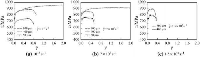

Shear stress-shear strain curves for different flow stress sizes

(ii):

Failure strain size effect: in Fig. 5, the failure strains for different specimens decrease as the strain rate increases. Failure strain of the material also has the size effect phenomenon.

Fig. 5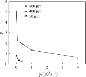

Failure strain versus strain rate curves

2.2 Regression of material constitutive model

Material constitutive model is that the flow stress of the material is a function of strain, strain rate, temperature, and other macroscopic thermodynamic parameters that produce heat. This model is the prerequisite for the metal plastic numerical analysis. Johnson–Cook (JC) constitutive model was proposed in 1983 by Johnson and Cook [7], and is used to describe mechanical behavior of a material with large deformation under high temperature and high strain rate conditions. Because of its simplicity, and easy to use, it is widely used in the industry. The original expression of the JC model is

$$ \tau = (A + B\gamma ^{n} )\left( {1 + C{\text{ln}}\dot{\gamma }^{*}} \right)\left( {1 - T^{*m} } \right) , $$

(2)

where τ is shearing stress, $\dot{\gamma }$ shear strain rate, T temperature, and dimensionless shear strain rate.

According to the experimental data obtained from three different specimens, the modified JC constitutive model expressions, for shear band width of 800, 400, and 50 μm, are as follows

$$ \tau = (561.19 + 246.07\gamma ^{{0.3041}} )\left( {1 + 1.75{\text{e}}^{{ - 3}} \dot{\gamma }^{{0.1436}} {\text{ln}}\frac{{\dot{\gamma }}}{{\dot{\gamma }_{0} }}} \right), $$

(3)

$$ \tau = (658.35 + 375.17\gamma ^{{0.3582}} )\left( {1 + 2.06{\text{e}}^{{ - 5}} \dot{\gamma }^{{0.5945}} {\text{ln}}\frac{{\dot{\gamma }}}{{\dot{\gamma }_{0} }}} \right) , $$

(4)

$$ \tau = (779.45 + 138.01\gamma ^{{0.2807}} )\left( {1 + 1.75{\text{e}}^{{ - 6}} \dot{\gamma }^{{0.6357}} {\text{ln}}\frac{{\dot{\gamma }}}{{\dot{\gamma }_{0} }}} \right). $$

(5)

3 Multiphase model on interfacial heat transfer for water quenching

Process control and parameters in manufacturing are corresponding to boundary conditions in simulation. The precise description for boundary conditions determines the accuracy of modeling.

The cooling method is a key factor affecting certain material properties in heat treating processes. The heat transfer between workpiece and medium plays an important role in modeling physics. Traditionally empirical functions [8–10] regressed from experimental data are used as boundary conditions. It uses a simple number or curves, like HTC, thus greatly simplifying the phenomena appearance during the process. The researchers [11–14] have integrated CFD theory with process analysis and tried to do a comprehensive modeling with workpiece and quenchant being regarded as a whole. It goes smoothly for gas quenching because of its feature of a single phase flow. However it turns out a totally different result for water quenching.

Water quenching is an unstable physical process with complex phase change of vaporization and happening fast within seconds. High cooling rate, large temperature gradient, two-phase interaction, phase change and fluid–solid conjugate heat transfer bring the difficulties into the modeling work. To overcome these difficulties, researchers have developed a water–vapor two-phase model [15] that is based on Eulerian–Eulerian multiphase flow theory.

3.1 Model for water quenching

The heat transfer in solid workpiece is governed by using heat conduction equation

$$ \frac{\partial \rho h}{\partial t} = \nabla (\lambda \nabla T) + S_{{_{\rm S} }} , $$

(6)

where $\rho$ is density, λ thermal conductivity, h enthalpy, t time, T temperature, and S _S source term.

Wall boiling starts when the wall temperature achieves a high value to initiate the activation of wall nucleation sites. A model is used by Kurul and Podowski [16] for formulating wall boiling. With it, only a few parameters, e.g., wall nucleation site density, bubble departure diameter, bubble detachment frequency, have to be given. The liquid water is set as continuous fluid, and the water vapor as dispersed phase.

The inhomogeneous particle model for interfacial transfer between continuous water and dispersed vapor particles has been chosen [17]. For interphase momentum transfer, the Schiller Naumann model [18] is chosen based on assumption that the interaction between bubbles is neglected. The drag coefficient for flow past spherical particles, $C_{{\text{d}}}$, is shown as

$$ C_{{\text{d}}} = \frac{{24}}{{Re}}(1 + 015Re^{{0.687}} ) $$

(7)

for interphase mass transfer, the mass flux can be derived from heat balance as

$$ \dot{m}_{{{\text{w,v}}}} = \frac{{q_{{\text{w}}} + q_{{\text{v}}} }}{{H_{{\text{v}}} - H_{{\text{w}}} }}, $$

(8)

where q _w and q _v are the heat flux from interface to water phase and vapor respectively, and H _v and H _w are the enthalpy taken into the water and vapor due to the phase change.

For interphase heat transfer, Ranz Marshall model is used to define the heat resistance on continuous phase, water, and Zero Resistance model for vapor side.

A case study has been done with an aluminum cylinder sample of 10 mm in diameter and 19 mm in length. The cylindrical sample is placed at the center of the fluid domain.

3.2 Results and discussion

The simulation result is shown in the following figures. Figure 6 shows the sample temperature history. Even in this small part with a good thermal conductivity, the temperature difference between the hottest and coolest points reaches around 40 °C with Biot number of the sample being only 0.067. The curve for the lowest temperature is fluctuant in the first 3 s. Considering that the lowest temperature points exist on the solid surface, it means the extremely unstable heat transfer of vaporization.

Fig. 6

Simulated temperature history of sample

The temperature of sample and water domain changes with time and space. The distribution at the moment of t equal to1 s is shown in Fig. 7. The water temperature in most region is below 100 °C except a thin layer surrounding the sample with a high temperature and high volume fraction of vapor.

Fig. 7

Temperature distribution in water at t = 1 s

The transient HTC along the sample profile is displayed in Fig. 8. The curves in OA and BC region fluctuate, which may be caused by floating movement of vapor bubbles. At the beginning, like t equal to 0.2 s, the HTC varies very fast from top (BC) to bottom (OA). After a short period less than 0.3 s, it becomes much more stable and uniform.

Fig. 8

Calculated HTC distribution along the profile of sample

Figure 9 shows HTC curve calculated using lumped heat capacity method based on the highest temperature curve of sample. The HTC is low at high temperature stage, because the accumulation of a large amount of small bubbles separates solid and liquid, and blocks the fierce heat transfer. At middle temperature stage, HTC reaches the highest value due to bubble boiling. Afterwards, the convection dominates with a steady heat transfer. The problem is that the peak value of calculated HTC seems lower than the experimental data, and the further work needs to be done to build more precise model.

Fig. 9

Calculated HTC curve dependent on sample temperature

4 Discrete model for precision machining process in mesoscopic scale

Modeling for manufacturing processes, which is based on the understanding of physical mechanism of new methodologies, has been developed from macro-scale to micro. Researchers need to investigate the fundamentals in material behavior, microstructure evolution, and integrated multiphysics, as well as the assumptions thought to be plausible.

Traditionally the workpiece during macro-cutting can be regarded as a continuum. The metal machining process squeezes the workpiece with a certain depth and speed of cutting, and elastoplastic deformation occurs along the primary shear zone. At the same time, the slide between chip and workpiece generates the secondary shear zone with high temperature and high pressure. The strong thermal interaction during the cutting process generates surface residual stress as well as micro-cracks, affecting the integrity of the workpiece surface.

From mesoscopic point of view, a workpiece is composed of a distribution of randomly orientated grains. The cutting process (see Fig. 10) breaks down the grains and grain boundaries of the workpiece, and makes the chip and workpiece become separation at the tool edge.

Fig. 10

Mesoscopic cutting process

Different machining accuracy requires different physical analysis model, and traditional modeling is based on the assumption that material is a continuous medium. In the precision and ultra-precision machining, however, sometimes only a few grains are involved in the cutting process. Therefore, it is necessary to analyze the microscopic mechanisms of the material removal process.

Figure 11 is the microstructure photography for the AISI 1045 steel. The left graph shows that the microstructure of the steel of AISI 1045, in which hexagonally shaped black gray pearlite (grain) similar to a honeycomb structure, are inlaid in the gray ferrite (grain boundary). The magnified image is on the right, where the dimensions of the pearlite are approximately 10–100 μm, and the size of ferrite is about 10 μm.

Fig. 11

Actual phase diagram (AISI 1045)

According to the features of precision and ultra-precision machining process, a discrete material cutting model is established as shown in Fig. 12.

Fig. 12

Precision cutting discrete material model

During the metal cutting process, because the cutting materials are in high strain rate deformation state, the constitutive model describing the plastic deformation of the material is critical to the success of the metal cutting process simulation. Johnson–Cook constitutive model is widely used due to its simplicity. Johnson–Cook constitutive model is as follows

$$ \sigma = (A + B(\varepsilon _{p} )^{n} )\left( {1 + C\;{\text{ln}}\left( {\frac{{\dot{\varepsilon }^{p} }}{{\dot{\varepsilon }_{0}^{p} }}} \right)} \right)\left( {1 - \left( {\frac{{T - T_{0} }}{{T_{{\text{m}}} - T_{0} }}} \right)^{{\it{m}}} } \right) $$

(9)

where σ is the flow stress of the material, ε the plastic strain, $\dot{\varepsilon }$ the plastic strain rate, T deformation temperature, T _m the melting point of the material, T ₀ room temperature, $\dot{\varepsilon }_{0}$ the reference plastic strain rate, and A, B, C, m, n material parameters.

For a specific material, with the given parameters, as shown in Table 1, the material constitutive model is established.

Table 1 Constitutive model parameters for grain/grain boundary

Another important aspect is the failure model. Since the deformation of the plastic material is caused by the dislocations shearing, the failure model can be use of shear failure parameters, and elastic modulus, Poisson’s ratio, density, thermal conductivity, specific heat capacity, etc. should be precisely determined.

The simulation and experimental results of different cutting depths and chip shapes are shown in Fig. 13, in which the chip shapes are similar to each other, thus verifying the accuracy of the finite element model.

Fig. 13

Comparison between simulation and experimental results of different cutting depths

5 Conclusions

Numerical modeling, as a newly developed technique for process analysis, has gained a great achievement in both academic research and industrial applications in manufacturing field. Physics-based modeling can enhance the accuracy of simulation by providing precise material properties, boundary conditions, and physical models. Furthermore, by taking advantages of the advanced equipment for testing, observing, and designing the certain characteristics of materials and processes, models for manufacturing will be improved significantly and applied to industrial processes more widely.

References

Fleck NA, Muller GM, Ashby MF et al (1994) Strain gradient plasticity: theory and experiment. Acta Metall Mater 42(2):475–487
Stolken JS, Evans AG (1998) A microbend test method for measuring the plasticity length scale. Acta Mater 46(14):5109–5115
Vollertsen F, Biermann D, Hansen HN et al (2009) Size effects in manufacturing of metallic components. CIRP Ann-Manuf Technol 58(2):566–587
Hu CM, He HL, Hu SS (2003) A study on dynamic mechancial behaviors of 45 steel. Explos Shock Waves 2:188–192
Li GH, Wang MJ, Kang RK (2010) Dynamic mechanical properties and constitutive model of Fe-36Ni invar alloy at high temperature and high strain rate. Mater Sci Technol 6:824–828
Yu HQ, Cheng JD (1999) Metal forming principle. China Machine, Beijing
Johnson GR, Cook WH (1983) A constitutive model and data for metal subjected to large strains, high strain rates and high temperatures. In: Proceedings of the 7th international symposium on ballistics, The Hague, 19–21 April 1983
Totten GE, Bates C, Clinton N (1993) Handbook of quenchants and quenching technology. ASM International, Almere
Mackenzie DS, Totten GE (2000) Aluminum quenching technology: a review. Mater Sci Forum 331–337:589–594
Xiao B, Wang Q, Jadhav P et al (2010) An experimental study of heat transfer in aluminum castings during water quenching. J Mater Process Technol 210:2023–2028
Wu Z, Caliot C, Flamant G et al (2011) Numerical simulation of convective heat transfer between air flow and ceramic foams to optimise volumetric solar air receiver performances. Int J Heat Mass Transf 54:1527–1537
Pan JS, Wang J, Gu JF (2012) One of progress in heat treatment numerical simulation: numerical model of heat treatment with expanded solution domain. Heat Treat Met 37(1):7–13
MacKenzie DS, Kumar A, Metwally H et al (2009) Prediction of distortion of automotive pinion gears during quenching using CFD and FEA. J ASTM Int 6(1):1–10
Xiao BW, Wang QG, Wang G et al (2010) Robust methodology for determination of heat transfer coefficient distribution in convection. Appl Therm Eng 30:2815–2821
Wang G, Rong YM (2012) Multiphase model on interfacial heat transfer for water quenching of cylindrical sample. In: TMS 2012 Annual Meeting & Exhibition, Orlando, 11–15 March 2012
Kurul N, Podowski MZ (1991) On the modeling of multidimensional effects in boiling channels. In: ANS processing of the 27th national heat transfer conference, Minneapolis
Wang G, Rong YM (2012) CFD-based modeling on interfacial heat transfer for water quenching. In: TMS 2012, Orlando, 11–15 March 2012
Schiller L, Naumann A (1933) A drag coefficient correlation. VDI Zeits 77:318–320
Author information
Authors and Affiliations
Corresponding author
Rights and permissions
About this article
Cite this article
Wang, G., Rong, YM. Advances of physics-based precision modeling and simulation for manufacturing processes. Adv. Manuf. 1, 75–81 (2013). https://doi.org/10.1007/s40436-013-0005-6
Received:
Accepted:
Published:
Issue Date:
DOI: https://doi.org/10.1007/s40436-013-0005-6