
Abstract
Energy supply security is one of the strategic issues of all states. In Iran, about 35 % of the total energy is consumed by the residential and commercial sectors. According to the importance of residential and commercial sectors in energy consumption, this paper develops different models to analyze energy demand of residential and commercial sectors. The GA and PSO energy demand estimation models (GA-DEM, PSO-GEM), a suitable model for this study, is used to estimate future energy demand of the sectors. Energy demand of these sectors has been estimated in two various forms, exponential and linear models. These sectors consumption in Iran from 1967 to 2010 is considered as the case of this study. The available data are partly used for finding the optimal, or near-optimal values of the coefficient parameters (1967–2006) and partly for testing the models (2007–2010). Our results show that PSO-DEM exponential model with inputs including, value added of all economic sectors, value of made buildings, the population and the electrical and fuel appliance price index using the mean absolute percentage error on test data is the most suitable model. Finally, based on the best scenario, the energy demand of residential and commercial sectors is estimated 1718 mega barrel of crude oil equivalent (MBOE) (1 barrel = 0.159 m3) up to the year 2032.
Find the latest articles, discoveries, and news in related topics.Avoid common mistakes on your manuscript.
Introduction
The world is in an unstable condition in the area of energy consumption and production (Oecd/Iea 2014). Iran as a country with an area of 1,900,000 km2 and an approximate population of 76 million people is the fourth country (after Venezuela, Saudi Arabia and Canada) in terms of its crude oil resources (156.53 milliard barrels of crude oil equivalent) and gas condensation; this equals to 9 % of the world’s oil stores [1]. Iran’s four main energy-consuming sectors include: transport, industry, residential–commercial and agriculture; the consumption rates of each of these four sectors according to 2012 balance sheet of Iran were 47.6, 48.2, 64.4 and 7.5 million tons of crude oil equivalent, respectively (Moe [3]). So 34 % of energy consumption was allocated to residential and commercial sectors; furthermore, Iran’s per capita energy consumption in these sectors is 1.9 as much as the world’s average rate [2]. Consumed energies in the residential and commercial sectors include: crude oil and oil productions, natural gas, coal, combustible renewable resources and electricity; the consumption rate for each sector has been computed to be 8.39, 46.13, 0.01, 1.31 and 8.58, respectively. These values show a 9.5 % growth. Many of Iran’s oil and gas resources have spent their half-lives [3]. Energy consumption modeling and predicting are comprehensive subjects which have attracted the attention of many scientists and engineers and highlighted both energy production and energy consumption subjects [4]. Energy planning cannot be practiced without having an acceptable level of knowledge about energy consumption in the past, now and predicting the probable energy demand in the future [5]. The demand for energy is estimated based on economic and non-economic indices obtained, probably, via linear and nonlinear statistical and mathematical methods as well as simulated models. The nonlinear indices on the one hand and the demand for energy on the other hand have triggered the process of seeking intelligent solutions such as genetic algorithm, particle swarm optimization algorithm, fuzzy-based regression and neural networks [6].
In recent years, many studies have been carried out on intelligent algorithms in order to predict the demand for energy. In the following section, a number of the studies are presented.
Ozturk and coworkers developed a GA energy demand model (GA-DEM) to estimate energy demand based on economic indicators in Turkey [7]. In 2007, Toksari developed a model for predicting the demand of energy using an ant colony algorithm. He applied the growth of GDP as the first economic index on his model, and then presented three scenarios for predicting demand of energy from 2006 to 2025. Finally, the prediction results improved when they compared with Ministry of Energy and Natural Resources (MENR) [8]. In 2008, Ünler developed a particle swarm optimization energy demand (PSO-DEM) model to predict the demand for electricity in Turkey. He compared the obtained results with those derived from an ant colony algorithm. This indicated that the former method gives improved results than the latter [9]. Canyurt and Ozturk presented Turkey’s fossil fuels demand estimation models by using the structure of the Turkish industry and economic conditions based on GA [10]. In 2010, Al-Rashidi and Naggar estimated the maximum annual electricity load of Kuwait using PSO algorithm in order to predict the demand for energy. They showed that the proposed model has less error compared with classic regression models [11]. Lee and Tong used the data collection of 1990–2007 and predicted energy consumption rate in China using a gray hybrid model and genetic algorithm. They found that this combined method estimates the simulated values close to the actual ones [12]. Kıran et al. employed a combined approach in their study and estimated the annual energy demand of Turkey using PSO and ant colony algorithms. They considered GDP, population, import and export as the inputs of linear and second-ordered models and found that the second ordered form have better performance in different scenarios [13]. In the study of Bahrami et al. the short term demand for electricity load in Iran and US were predicted using a combined approach; PSO and neural network algorithms. They took into account weather information variables including temperature average, relative humidity average, wind speed average and information of previous electricity consumption as their model’s input and found that the combined model improves the prediction of electrical load [14]. Ardakani and Ardehali predicted the long term demand for electricity load in Iran and US using neural network and PSO algorithms. They considered GDP, energy import, energy export and population data from 1967 to 2009 and predicted demand of energy in the countries up to 2030 [15].
Objectives of study
This study presents the application of the PSO and GA methods for estimation and prediction of energy demand in residential and commercial sectors in Iran. The socio-economic indicators use in this study are value added of all economic sectors (total value added): the total value added minus that of the oil sector, National Income, Gross fixed capital formation for the constructions, value of made buildings, Population, Total Number of Households, Total Labor, Population minus the Labor, Electrical and Fuel Appliance Price index, Energy Price index adjusted by the General Price Index and Consumer Energy (Fuel) Price Index. The models developed in two forms (exponential and linear) are applied to prediction of energy demand in residential and commercial sectors in Iran. The objective of the study is answering these questions: (1) what is the appropriate scenario to predict energy demand in residential and commercial sectors of Iran? (2) How much will the annual demand for energy in residential and commercial sectors be up to 2032?
This study has been structured in fo ur sections. the first section "Introduction" explains the theoretical fundamentals of genetics and particle swarm optimization algorithms in brief. The second section discusses "Methodology", third section, presents the "Results and discussion". Fourth section presents "Conclusion".
Genetic algorithms
The Genetic algorithm is actually the most famous type of evolutionary algorithms created and developed by John Holland et al. In the 1960s, Rechenberg introduced the evolutionary computing idea in a book titled as “Evolution strategies”. Research on genetic algorithm was exactly initialized after research on artificial neural networks. Both fields have been inspired by biological systems as a motivating and computing model. It is an iterative algorithm and in any iteration, it deals with a single or several different solutions. In genetic algorithm the searching process is initialized with a population of primary random solutions. If final criteria are not satisfied, three different operators—reproduction, mutation and crossover—will apply to update the population. Any iteration of the three mentioned operators is considered as a generation. Since the solutions of this algorithm are very similar to natural chromosomes and the operators work similar to genetic operators, this algorithm has been named the “genetic algorithm”. In fact, genetic algorithm searches solution space by repeating three simple steps. In the first step, it assesses a group of points named as population, in accordance with the target function. In the second step, it selects some points as the nominees of the problem’s solutions based on the assessments of the previous step and in the third step; genetic operators are applied to the selected nominees in order to create the population of the next generation. This process is repeated until the final criterion is achieved. This criterion is achieved when an acceptable solution is obtained or the maximum number of a generation is repeated [16, 17].
Particle swarm optimization algorithm
Particle swarm optimization is an evolutionary algorithm for optimizing functions. It has been designed based on the social behavior of birds. It was introduced by Kennedy in 1995. In this algorithm a group of particles (as the variables of an optimization problem) is dispersed in the search environment. Obviously, some particles will occupy better positions than the others. Therefore, according to aggregate particle behaviors, other particles will try to raise their position to the prior particle positions. In this method, the position change is done based on every particle’s experience obtained in previous motions as well as the experiences of neighboring particles. In fact, every particle is aware of its priority/nonpriority over neighboring particles as well as over the whole group [17].
In the functional model, the particles move in search space. Particle (i) is detected by its location (x i ) and displacement vector (v i ). Particle displacement in each iteration is described by Eq. (1):
where t indicates the number of current iterations.
Each particle makes use of the following information to change its location and velocity:
-
1.
The global best (gbest) location which is known to everybody. As each particle detects the best new location, it sends the related information to other particles.
-
2.
The personal best (pbest) location is the best solution a particle has ever experienced.
All particles begin to be influenced by the global best location until they reach the location. Particles move around the general best location in the search space. They do not search the rest of the space and this is called the convergence phenomenon.
Equation (2) derives the velocity vector from the addition of initial velocity vectors of gbest and pbest.
where c 1 and c 2 parameters indicate the rate of dependency on individual intelligence. The more the c 1 increases, the higher the pbest contribution will become in the velocity equation and the particle’s tendency will increase to determine its route based on its own experiences. On the contrary, by an increase in c 2, the tendency of the particle to join the group will increase.
In order to prevent explosive velocity on one hand and convergence on the other hand, the inertia coefficient (w) a number from the interval [0–1] is used according to Eq. (3). Therefore, the particle velocity will gradually decrease and reach 0 in approximation to the global best location. Rand coefficients of random numbers are uniformly distributed between 0 and 1, causing the particle search for its own route instead of moving on a straight line.
where maxiter is the maximum number of iterations and iter is the current iteration counter.
Figures 1 and 2 show the flow charts of the mentioned algorithms, respectively.

GA flow chart

PSO flow chart
Methodology
Data collection and pre-processing
The data in this study, collected from the annual reports of Central Bank, Ministry of Energy and Ministry of Petroleum of Iran (2010). These data were divided into the education data (1976–2007) and the test data (2008–2010). First of all, to initialize the computing process using GA and PSO algorithms the data were converted to normal data with a value between 0 and 1. This conversion was performed using Eq. (4).
where z, x, µ and δ are normal distribution function, variable’s value, mean and standard deviation data, respectively.
Development of different scenarios for predicting energy demand of residential and commercial sectors
As it was mentioned before, this research assesses different scenarios with different inputs and selects the best scenario. After studying different research and acquiring experts’ opinions, the model’s variables, including input and output variables [18] were selected as follows.
Output variable
Annual energy consumption in residential and commercial sectors was selected as the output variable of the model; Fig. 3 shows an energy consumption rate in residential and commercial sectors from 1967 to 2010.

Energy consumption in residential and commercial sectors
Input variables
-
❖ Value added
The value added is associated with four economic sectors: oil sector, industry plus mining, commercial and agriculture. It can serve as an appropriate index for measuring income/welfare of an individual or a family. Regarding oil sector, income does not directly affect consumption. Therefore, the value added is divided into two groups: Oil and non oil sectors. Thus, this section’s variable is considered as follows. The unit of each variable is determined and its symbol is shown inside parentheses.
-
✓ Value added of all economic sectors (total value added): VAT [103 × BIRR]
-
✓ The total value added minus that of the oil sector: VAN [103 × BIRR]
-
✓ National income: YNI [BIRR]
Figure 4 shows the variables’ values from 1967 to 2010.
Fig. 4 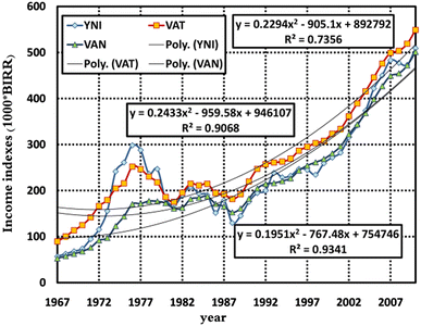
Income Index
-
-
❖ Building
The investment in building sector or the worth of the constructed buildings shows that how many buildings are added annually to previous buildings or in other words, how much energy is required for cooling, heating and ventilation systems of the buildings. On this basis, two variables were considered for this sector:
-
✓ Gross fixed capital formation for the constructions: INVC [103 × BIRR]
-
✓ Value of made buildings: BLD [103 × BIRR]
Figure 5 shows the variables’ values from 1967 to 2010.
Fig. 5 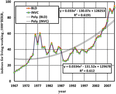
Living and Work Space Index
-
-
❖ Population and work force
Undoubtedly, population plays a significant role in the energy consumption of residential and commercial sectors. However, the work force is a part of out of home population who affect energy consumption of the sector. Therefore, the influential variables of this section are classified as follows:
-
✓ Population: PO [million]
-
✓ Total number of households: HNT [million]
-
✓ Total labor: LT [million]
-
✓ Population minus the labor: PNL [million]
Figure 6 shows the variables’ values from 1967 to 2010.
Fig. 6 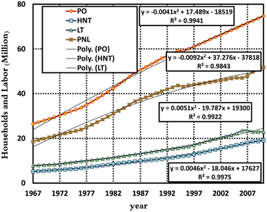
Population and Work Force Index
-
-
❖ Price
The following variables were considered for the price index:
-
✓ Electrical and Fuel Appliance Price index: PAPL
-
✓ Consumer Energy (Fuel) Price Index: PFC
-
✓ Energy Price index adjusted by the General Price Index: PFPG.
It should be noted that the consumer may not reduce his/her consumption rate even in the event of a price increase, because the residential and commercial sectors energy is irreplaceable. The consumer, in fact, determines his/her consumption level based on the price of different fuels not based on its previous price. Therefore, the index of energy price adjusted by general price has been taken into account. Figures 7, 8 and 9 show the variables’ values from 1967 to 2010, respectively.
Fig. 7 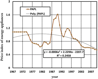
Electrical Appliances and Fuel Price Index (normalized data)
Fig. 8 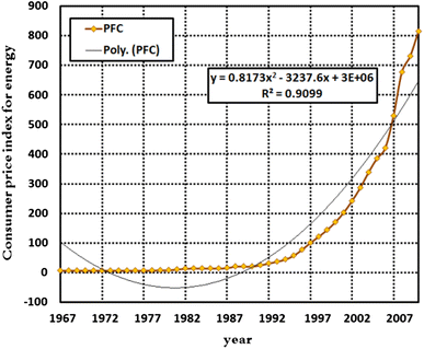
Energy Price for Consumer Index (1997 = 100)
Fig. 9 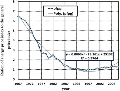
Energy Price Adjusted by General Price Index
-
-
❖ For each socio economic indicator, the polynomial trend lines are fitted to the observed data with the highest R 2 values.


Any of the above mentioned input variables can be considered as an input variable. For example, the value added of all economic sectors, total value added minus oil sector and national income can be considered as an input variable. Different scenarios assume each of the variables as an input variable and investigate the test data and finally select the best scenario. Different input variables lead to (3*2*4*3=72) parallel models were obtained by combining the variables as different scenarios. Table 1 shows the models.
Problem definition
This study presents the application of the PSO and GA methods to estimate and predict residential and commercial sectors energy demand in Iran. The fitness function, F(T), takes the following form Eq. (5):
where t, n, sim(t) and RE(t) are the time, number of variables, simulated value and actual value of data, respectively.
Forecasting of energy demand in residential and commercial sectors based on economic indicators was modeled by using both linear and exponential models. Moreover, a constant signal and a dummy variable, which indicates the especial conditions of the country in the revolving years and the ending years of the war, can be added to the model.
The linear form of Eq. (6) for the demand estimation models is written as:
The exponential form of Eq. (7) for the demand estimation models is written as:
Here, α, β, γ and c are the coefficients derived from the genetic algorithm. X(t) stands for the model’s input variable in terms of time. Y(t) stands for the model’s output variable showing the energy consumption of residential and commercial sectors by one mega ton of crude oil equivalent. Moreover, a constant signal and a dummy variable, which indicates the especial conditions of the country in the revolution years and the ending years of the war, can be added to the model.
A total of 288 models were designed using GA and PSO algorithms and their validity were confirmed using root mean square error (RMSE) fitness function and mean absolute percentage error (MAPE) as shown in Eqs. (8) and (9), respectively.
Here y actual and y estimated are the actual value and estimated value, respectively.
The GA and PSO algorithms were coded with MATLAB R2013a. The convergence of the objective function and sensitivity analysis were examined for varying user-specified parameters of GA (population size, methods of selection, reproduction, crossover, mutation and generation). Each user-specified parameter combination (algorithm) was tested 100 times. It was found that in GA, the variations in population size, creation function, crossover fractions and mutation scale had most effect on fitness function while number of generation had minimum effect on it.
The best results of the GA-DEM and PSO-DEM models are performed using the following user-specified parameters:
“GA”:
-
Population: (population size: 150).
-
Population type: double vector, creation function: uniform).
-
Selection: (selection function: stochastic uniform).
-
Reproduction: (Elite count: 2.0, crossover fractions: 0.08).
-
Crossover: (crossover function: scattered).
-
Mutation: (mutation function: Gaussian, Scale: 1.0, Shrink: 1.0).
-
Stopping criteria: (generation: 100).
“PSO”:
-
Maximum iteration number (t): 100.
-
Particle size (n): 40.
-
Inertia weight (w): 0.6.
-
C 1 = C 2 = 2.
Results and discussion
Selecting the most appropriate model for predicting energy demand of residential and commercial sectors
After developing different scenarios and simulating them for 100 times, the following four models were selected, out of 288 models, as the best models of linear and exponential states:
The linear Eq. (10) was estimated by the genetic algorithm:
The exponential Eq. (11) was estimated by the genetic algorithm:
The linear Eq. (12) was estimated by the particle swarm optimization algorithm:
The exponential Eq. (13) was estimated by the swarm particle optimization:
where ER is energy consumption in residential–commercial sector, VAT is value added of all economic sectors (total value added), INVC is gross fixed capital formation for the constructions, BLD is value of made buildings, PO is population, PNL is Population minus the labor, PFC, Consumer Energy (Fuel) Price Index, PAPL is Electrical and Fuel Appliance price index.
Figures 10, 11, 12 and 13 show the curves of the best simulated states of the above four equations.

The best GA-DEM linear model derived from GA algorithm

The best GA-DEM exponential model derived from GA algorithm

The best PSO-DEM linear model derived from PSO algorithm

The best PSO-DEM exponential model derived from PSO algorithm
To select the best model, the test data were assessed using Eqs. (8) and (9). Tables 2 and 3 show the results. According to the results, the best scenario for predicting the energy demand of residential and commercial sectors of Iran is derived from the exponential model simulated by a PSO algorithm.
The results indicate that among the above possible states, the exponential model derived from PSO algorithm is the best model with the minimum MAPE and RMSE for predicting the future trend of energy demand of Iran.
For the best results of GA, the average relative errors on testing data were 2.68 and 3.25 % for GA-DEMexponential and GA-DEMlinear, respectively. The corresponding value for PSO was 1.97 and 3.07 % for PSO-DEMexponential and PSO-DEMlinear, respectively.
Validations of models show that PSO-DEM and GA-DEM are in good agreement with the observed data but PSO-DEMexponential outperformed other models presented here.
These steps are used for forecasting Iran’s energy demand in the years 2013–2032.
Comparison between presented models in the literature review and presented models in this study are shown in Table 4.
Prediction of Energy demand of residential and commercial sectors up to 2032
With regard to Eq. (13), the PSO-DEMexponential model simulated by the PSO algorithm was selected as the best scenario. Therefore, the energy demand of residential and commercial sectors was predicted up to 2032. According to Fig. 14, the energy demand of these sectors will have an increasing trend up to 2032 and grow up to 1718 mega barrel of crude oil equivalent. This value has an exponential growth with the highest R 2 (root mean square) level up to the year 2032.

The prediction of energy consumption in residential and commercial sectors up to 2032
Conclusion
In this study, estimation of Iran’s residential and commercial sectors demand with a model based on GA and PSO are suggested via considering value added of all economic sectors (total value added): the total added minus that of the oil sector, National Income, Gross fixed capital formation for the constructions, value of made buildings, Population, Total number of households, Total Labor, Population minus the Labor, Electrical and Fuel Appliance price index, Energy price index adjusted by the General Price Index and Consumer Energy (Fuel) Price Index socio-economic indicators. Two forms (linear and exponential) of the GA-DEM and PSO-DEM models are developed to meet the volatility of economic indicators. 45 years data (1967–2010) is used to show the availability and advantages of the proposed approach. As it was mentioned before, this research assesses different models with different inputs and selects the suitable model. In addition, the following main conclusions may be drawn in this study:
-
While the largest deviation were 3.25 % for linear form GA-DEM, the largest deviation was 2.68 % for exponential form GA-DEM and 3.07 % for linear form PSO-DEM, the largest deviation was 1.97 % for exponential form PSO-DEM in modeling with 45 years data (1967–2010). Then, it was observed that exponential PSO-DEM provided the best fit solution than a linear form due to the fluctuations of the economic indicators.
-
The PSO-DEM exponential model (suitable model) was evaluated among 72 models were made with the following inputs: value added of all economic sectors (total value added), Consumer Energy (Fuel) Price Index, Population minus the Labor and value of made buildings.
-
The energy demand of these sectors will have an increasing trend up to 2032 and grow up to 1718 mega barrel of crude oil equivalent. This value has an exponential growth with the highest R 2 (root mean square) level up to the year 2032.
-
The prediction of the energy demand in other sectors using the method presented here is highly recommended. However, other meta-heuristic algorithms can be used to predict the energy demand of residential and commercial sectors and the obtained results can be compared with those created for this study. It is also anticipated that this study may be helpful in developing, a highly applicable and productive planning for energy policies.
Abbreviations
- PSO:
-
Particle swarm optimization algorithm
- GA:
-
Genetic algorithm
- PSO-DEM:
-
The PSO energy demand estimation
- GA-DEM:
-
The GA energy demand estimation
- MAPE:
-
Mean absolute percentage error
- RMSE:
-
Root mean square error
- MBOE:
-
Mega barrel of crude oil equivalent
- MTOE:
-
Mega tons of crude oil equivalent
- MENR:
-
Ministry of Energy and Natural Resources
- Gbest:
-
The global best location
- Pbest:
-
The personal best location
References
Assareh, E., Behrang, M., Assari, M., Ghanbarzadeh, A.: Application of PSO (particle swarm optimization) and GA (genetic algorithm) techniques on demand estimation of oil in Iran. Energy 35(12), 5223–5229 (2010)
Karbassi, A., Abduli, M., Mahin Abdollahzadeh, E.: Sustainability of energy production and use in Iran. Energy Policy 35(10), 5171–5180 (2007)
(MOE) M.o.E.: Energy balance annual report. Ministry of Energy, Tehran, Iran (2012)
Ozturk, H.K., Ceylan, H.: Forecasting total and industrial sector electricity demand based on genetic algorithm approach: Turkey case study. Int. J. Energy Res. 29(9), 829–840 (2005)
Sözen, A., Gülseven, Z., Arcaklioğlu, E.: Forecasting based on sectoral energy consumption of GHGs in Turkey and mitigation policies. Energy Policy 35(12), 6491–6505 (2007)
Azadeh, A., Tarverdian, S.: Integration of genetic algorithm, computer simulation and design of experiments for forecasting electrical energy consumption. Energy Policy 35(10), 5229–5241 (2007)
Ozturk, H.K., Canyurt, O.E., Hepbasli, A., Utlu, Z.: Residential-commercial energy input estimation based on genetic algorithm (GA) approaches: an application of Turkey. Energy Build. 36(2), 175–183 (2004)
Toksarı, M.D.: Ant colony optimization approach to estimate energy demand of Turkey. Energy Policy 35(8), 3984–3990 (2007)
Ünler, A.: Improvement of energy demand forecasts using swarm intelligence: The case of Turkey with projections to 2025. Energy Policy 36(6), 1937–1944 (2008)
Canyurt, O.E., Ozturk, H.K.: Application of genetic algorithm (GA) technique on demand estimation of fossil fuels in Turkey. Energy Policy 36(7), 2562–2569 (2008)
AlRashidi, M., El-Naggar, K.: Long term electric load forecasting based on particle swarm optimization. Appl. Energy 87(1), 320–326 (2010)
Lee, Y.-S., Tong, L.-I.: Forecasting energy consumption using a grey model improved by incorporating genetic programming. Energy Convers. Manag. 52(1), 147–152 (2011)
Kıran, M.S., Özceylan, E., Gündüz, M., Paksoy, T.: A novel hybrid approach based on particle swarm optimization and ant colony algorithm to forecast energy demand of Turkey. Energy Convers. Manag. 53(1), 75–83 (2012)
Bahrami, S., Hooshmand, R.-A., Parastegari, M.: Short term electric load forecasting by wavelet transform and grey model improved by PSO (particle swarm optimization) algorithm. Energy 72, 434–442 (2014)
Ardakani, F., Ardehali, M.: Long-term electrical energy consumption forecasting for developing and developed economies based on different optimized models and historical data types. Energy 65, 452–461 (2014)
Talbi, E.-G.: Metaheuristics: from design to implementation, vol. 74. Wiley, UK (2009)
Haupt, R.L., Haupt, S.E.: Practical genetic algorithms. Wiley, UK (2004)
Shakouri, G.H., Kazemi, A.: Energy demand forecast of residential and commercial sectors: Iran case study. In: Proceedings of the 41st international conference on computers and industrial engineering 23–25 October, Los Angeles, CA, USA (2011)
Author information
Authors and Affiliations
Corresponding authors
Rights and permissions
Open Access This article is distributed under the terms of the Creative Commons Attribution 4.0 International License (http://creativecommons.org/licenses/by/4.0/), which permits unrestricted use, distribution, and reproduction in any medium, provided you give appropriate credit to the original author(s) and the source, provide a link to the Creative Commons license, and indicate if changes were made.
About this article

Cite this article
Nazari, H., Kazemi, A., Hashemi, MH. et al. Evaluating the performance of genetic and particle swarm optimization algorithms to select an appropriate scenario for forecasting energy demand using economic indicators: residential and commercial sectors of Iran. Int J Energy Environ Eng 6, 345–355 (2015). https://doi.org/10.1007/s40095-015-0179-8
Received:
Accepted:
Published:
Issue Date:
DOI: https://doi.org/10.1007/s40095-015-0179-8